5.1.3. Method of solution
ORIGEN solves the system of ordinary differential equations (ODEs) that describe nuclide generation, depletion, and decay,
where
\(N_{i}\) = amount of nuclide i (atoms),
\(\lambda_{i}\) = decay constant of nuclide i (1/s),
\(l_{\text{ij}}\) = fractional yield of nuclide i from decay of nuclide j,
\(\sigma_{i}\) = spectrum-averaged removal cross section for nuclide i (barn),
\(f_{\text{ij}}\) = fractional yield of nuclide i from neutron-induced removal of nuclide j,
\(\Phi\) = angle- and energy-integrated time-dependent neutron flux (neutrons/cm2-s), and
\(S_{i}\) = time-dependent source/feed term (atoms/s).
Note that Eq. (5.1.1) has no spatial dependence and can be interpreted as either a solution at a point in space or the spatial average over some volume. The latter interpretation is preferred here, such that \(\Phi\) is the spatially averaged neutron flux magnitude, and all energy-dependence is embedded in the one-group flux-weighted average cross sections \(\sigma_{i}\) and reaction yields \(f_{\text{ij}}\). Eq. (5.1.1) is conveniently written in matrix form as
with a \(\mathbf{A}\) commonly referred to as the “transition matrix.” The representation of the transition matrix as \(\mathbf{A = A}_{\sigma}\Phi\mathbf{+}\mathbf{A}_{\lambda}\), where \(\mathbf{A}_{\sigma}\) is the part of the transition matrix containing reaction terms and \(\mathbf{A}_{\lambda}\) is the part containing decay terms, is convenient, as the numerical solution of this system of ODEs holds the reaction, flux, and feed terms constant over step \(n\),
over time step \(t_{n - 1} \leq t \leq t_{n}.\)
Adding a continuous removal process described with rate constant \(\lambda_{i,rem}\) simply modifies the decay constant, \(\lambda_{i} \rightarrow \lambda_{i} + \lambda_{i,rem}\), whereas a continuous feed process defines a nonzero component of the \({\overrightarrow{S}}\) vector.
ORIGEN can also compute the alpha, beta, neutron, and gamma emission spectra during decay. For the “stand-alone” ORIGEN calculations described here, the transition matrix is loaded from an ORIGEN binary library file (f33), which uses sparse-matrix storage to store one or more transition matrices. The f33s may be created using COUPLE, saved from TRITON depletion calculations, or interpolated using ARP from a set of precompiled f33s distributed with SCALE.
Results from ORIGEN calculations may be stored on a binary concentration file (f71), which facilitates transfer of isotopics to other codes in SCALE. The f71 file can also store calculated emission spectra. Within ORIGEN, the f71 can be used to restart calculations from an existing set of compositions.
5.1.3.1. Methodology
This section describes the methodology used in performing the following main functions:
generation of problem-dependent transition matrices,
solution of the system of depletion/decay equations,
conversion from power to flux (important for reactor applications),
calculation of emission spectra,
interpolation of pregenerated sets of transition matrices, and
calculation of sensitivity coefficients.
5.1.3.1.1. Generation of Problem-dependent Transition Matrix
In the transition matrix \(\mathbf{A}\) from Eq. (5.1.2), each matrix element \(a_{\text{ij}}\) is the first-order rate constant for the formation of nuclide i from nuclide j given below.
The transition matrix coefficients for decay and reaction transitions are stored separately and reaction transitions are always stored with \(\Phi = 1\) and later during solution of the system, depending on the step-average flux level the actual transition matrix \({\mathbf{A}_{n}\mathbf{= A}}_{\sigma,n}\Phi_{n}\mathbf{+}\mathbf{A}_{\lambda}\) is reconstructed using step-average flux, \(\Phi_{n}\).
The decay coefficients \(l_{\text{ij}}\lambda_{j}\) and \(\lambda_{i}\) are generated directly from ORIGEN decay resource data. The reaction coefficients \(f_{\text{ij}}\sigma_{j}\) and \(\sigma_{i}\) are generated using the following two-stage procedure.
Calculate all removal cross sections \(\sigma_{i}\) and yields \(f_{\text{ij}}\), including isomeric branching ratios and fission yields, by folding provided flux spectrum \(\phi^{g}\) with multigroup cross sections from the ORIGEN reaction resource and energy-dependent fission yield data from the ORIGEN yield resource.
Overwrite specific removal cross sections and yields based on a provided multigroup cross section library (see the SCALE Nuclear Data Libraries chapter) and/or user-provided one-group cross sections and yields.
The second stage is optional, but it is important for cases which there is significant self-shielding because ORIGEN’s reaction resource assumes infinite dilution for its multigroup data. The decay, reaction, and yeld resources mentioned here are described in the ORIGEN Data Resources chapter. The collapse to a one-group cross section in either stage is given by
for reaction type \(r\), nuclide \(i\), and provided multigroup flux \(\phi^{g}\). Different reaction types are recognized by their ENDF MT numbers [SCALE Cross Section Libraries chapter] on the appropriate data resource For example, MT=16 is \(\left( n,2n \right),\) and MT=107 is \(\left( n,\alpha \right)\). The removal cross section \(\sigma_{i}\) is simply calculated as the sum over all relevant reactions for a particular nuclide, \(\sigma_{i} = \ \sum_{r}\sigma_{\text{ri}}\). This type of reaction-dependent multigroup data may be contained in either the data sources available in stage 1 or 2 above. However, only two types of data are expected to be available in stage 1 reaction resource data: (1) isomeric branching and (2) fission yields.
The energy-dependent isomeric branching that describes the yield of each excited level (metastable state) of a daughter nucleus is calculated in a similar way,
where \(m\) indicates the possible metastable states and the fractions always satisfy \(\sum_{m}f_{\text{rim}}^{\ } = 1\).
Fission product yields are typically tabulated at discrete neutron energies such as thermal (0.0253 eV), fission (500 keV), and high energy (14 MeV). The yield for each fissionable nuclide is calculated in stage 1 by linearly interpolating the tabulated data using the computed average energy of fission,
where \(\sigma_{\text{fi}}^{g}\) is the multigroup fission cross section, and \({\overline{E}}^{g}\) is the average energy in the group (simple midpoint energy used). In addition to generating transition data for daughter/residual nuclides, the coefficients for byproducts such as He-4/\(\alpha\) byproducts from \(\left( n,\alpha \right)\) reactions are also retained in the transition matrix and associated to an appropriate nuclide in the system: hydrogen, deuterium, tritium, 3He, or 4He.
5.1.3.1.2. Solution of the Depletion/Decay Equations
ORIGEN includes two solver kernels that can solve the depletion/decay equations of Eq. (5.1.3):
a hybrid matrix exponential/linear chains method (MATREX) and
a Chebyshev Rational Approximation Method (CRAM).
They are described in the following sections.
5.1.3.1.2.1. MATREX
Referring to the system of ODEs shown in Eq. (5.1.2) and setting the external feed/source \(S\left( t \right) = 0\), there is a formal solution by matrix exponential (an analog to the solution of a single ODE of this type by exponential),
where \(\overrightarrow{N}\left( 0 \right)\) is a vector of initial nuclide concentrations, by defining the series expansion of \(exp(\mathbf{A}t\mathbf{)}\) to be
with \(\mathbf{I}\) the identity matrix. Eq. (5.1.8) and Eq. (5.1.9) describe the matrix exponential method, which yields a complete solution to the problem. However, in certain instances related to limitation in computer precision, difficulties occur in generating accurate values of the matrix exponential function. Under these circumstances, alternative procedures using either the generalized Bateman equations [ORIGEN-Bat10] or Gauss-Seidel iterative techniques are applied. These alternative procedures will be discussed in further sections.
A straightforward solution of Eq. (5.1.8) and Eq. (5.1.9) would require storage of the complete transition matrix. To avoid excessive memory requirements, a recursion relation has been developed. Substituting Eq. (5.1.9) into Eq. (5.1.8),
one may recognize a recursion relation for a particular nuclide, \(N_{i}(t)\).
where the range of indices, j, k, m, is 1 to M for matrix \(\mathbf{A}\) of size \(M \times M\). The result is a series of terms that arise from the successive post-multiplication of the transition matrix by the vector of nuclide concentration increments produced from the computation of the previous terms. Within the accuracy of the series expansion approximation, physical values of the nuclide concentrations are obtained by summing a converged series of these vector terms. By defining the terms \(C_{i}^{n}\left( t \right)\) as
the solution for \(N_{i}\left( t \right)\) is given as
The use of Eq. (5.1.12) and Eq. (5.1.13) requires storage of only two vectors–\({\overrightarrow{C}}^{n}\) and \({\overrightarrow{C}}^{n + 1}\) —-in addition to the current value of the solution. However, the series summation solution in Eq. (5.1.13) is not valid until a finite limit is identified which can achieve a reasonable accuracy, i.e.,
where \(n_{\text{term}}\) is the number of terms and \(\epsilon_{\text{trunc}}\) is the truncation error. The key is to split the nuclides into two sets: those that are long-lived and permit a rapid, accurate solution via Eq. (5.1.14), and those that are short-lived and require an alternate solution.
Solution for Long-Lived Nuclides
This section describes the various tests used to ensure that the summations indicated in Eq. (5.1.14) do not lose accuracy due to large changes in magnitudes or small differences between positive and negative rate constants. Nuclides with large rate constants (short-lived) are removed from the transition matrix and treated separately. For example, in the decay chain \(\mathrm{A\rightarrow B \rightarrow C}\), if the decay constant for B is large, a new rate constant is inserted in the matrix for \(\mathrm{A \rightarrow C}\). This technique was originally employed by Ball and Adams [ORIGEN-BA67]. The key to determining which transitions should be removed involves calculation of the matrix norm. The norm of matrix \(\mathbf{A}\) is defined by Lapidus and Luus [ORIGEN-LL67] as being the smaller of the maximum-row absolute sum and the maximum-column absolute sum,
To maintain precision in performing the summations of Eq. (5.1.14), the matrix norm is used to balance the user-specified time step, t, with the precision associated with the word len>h employed in the machine calculation. The constraint on the matrix norm has been chosen as
The remainder of this section shows that this constraint serves two purposes.
It allows reasonable accuracy for a reasonable number (20–60) of matrix exponential terms.
It defines what “short-lived” means over a particular time step, dictating which concentrations must be solved by alternate means.
A relationship between m digits of machine precision and p significant digits required in all results can be stated by the following inequality:
In this particular series, the relationship may be represented as
or alternatively,
Lapidus and Luus have shown that the maximum term in the summation for any element in the matrix exponential function cannot exceed \(\frac{\left( \left\lbrack \mathbf{A} \right\rbrack t \right)^{n}}{n!},\ \)where \(n\) is the largest integer not larger than \(\left\lbrack \mathbf{A} \right\rbrack t\). For the constraint in Eq. (5.1.16), this yields n=13 and yields limit \(\frac{\left( \left\lbrack \mathbf{A} \right\rbrack t \right)^{n}}{n!} \approx 10^{5}\). With \(e^{\left\lbrack \mathbf{A} \right\rbrack t} \approx 10^{6}\) and standard double precision with m=16, Eq. (5.1.19) evaluates to \(10^{11} \leq 10^{16 - j}\), which indicates that five significant figures will be maintained in values as small as 10–6. The number of terms required to converge the matrix exponential series can be investigated by a plot of the \(\frac{\left| \left\lbrack \mathbf{A} \right\rbrack t \right|^{n}}{n!}e^{\left\lbrack \mathbf{A} \right\rbrack t}\) as a function of term index n in Eq. (5.1.19), as shown in Fig. 5.1.1
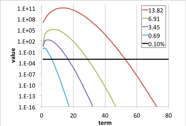
Fig. 5.1.1 Values of terms in series for various values of the matrix norm.
The intersection between the black line in Fig. 5.1.1 and the various curves indicates the number of terms needed to achieve \(\epsilon_{\text{trunc}} \leq 0.1\%\). For example, with \(\left\lbrack \mathbf{A} \right\rbrack t = 13.8155\), \(n_{\text{term}} = 54\) is required, and with \(\left\lbrack \mathbf{A} \right\rbrack t = 13.8155/2\), approximately \(n_{\text{term}} = 29\) is required. This behavior has been used to develop the heuristic
Thus it has been shown that the limit imposed in Eq. (5.1.16) leads to a maximum of \(n_{\text{term}} = 54\) terms with \(\epsilon_{\text{trunc}} \leq 0.1\%\).
It remains to be shown that any arbitrary system can be modified so that it does not violate Eq. (5.1.16). Because the time step \(t\) is provided and fixed, \(\left\lbrack \mathbf{A} \right\rbrack t \leq \ - 2\ \ln(0.001)\) cannot be satisfied unless the system is modified. The physical nature of the system leads to \(\max_{j}{\sum_{i}\left| a_{\text{ij}} \right|} \leq \max_{j}{2|a_{\text{jj}}|}\) based on production rates equal to loss rates when both parent and daughter nuclide are included in the system. The maximum column sum in Eq. (5.1.15) can then be bounded by twice the maximum diagonal term, \(\max_{j}{2|a_{\text{jj}}|}\). Using this upper limit as the matrix norm and substituting into Eq. (5.1.16) yields
Rearranging Eq. (5.1.21) leads to the condition
which is used to mark nuclide j as a short-lived nuclide for this time step, to be solved with linear chains instead of the series-based matrix exponential. An alternative interpretation of the short-lived condition can be made by rewriting Eq. (5.1.22) in terms of an effective half-life, \(t_{1/2} = \frac{\ln\left( 2 \right)}{|a_{\text{jj}}|}\), which results in \(t_{1/2} < \frac{{- ln}\left( 2 \right)}{\ln\left( 0.001 \right)}t \approx 0.1t\). In other words, when a nuclide’s effective half-life (including destruction by both decay and reaction mechanisms) is less than 10% of the time step, it can be considered short-lived.
Finally, as a note for applications where the nuclides of interest are in long transmutation chains, it has been found that the above algorithm may not yield accurate concentrations for those nuclides near the end of the chain that are significantly affected by those near the beginning of the chain. In these applications, specifying the minimum \(n_{\text{term}}\) as
where \(\Delta Z\) is the atomic number difference and \(\Delta A\) is the mass number difference, has been found to ameliorate the issue.
Solution for Short-Lived Nuclides
The condition in Eq. (5.1.22) forms the basis for declaring a nuclide short-lived, and its solution is found via solution of the nuclide chain equations. In conjunction with maintaining the transition matrix norm below the prescribed level, a queue is formed of the short-lived precursors of each long-lived isotope. These queues extend back up the several chains to the last preceding long-lived precursor. According to Eq. (5.1.22), the queues will include all nuclides whose effective half-lives are less than 10% of the time interval. A generalized form of the Bateman equations developed by Vondy [ORIGEN-Von62] is used to solve for the concentrations of the short-lived nuclides at the end of the time step. For an arbitrary forward-branching chain, Vondy’s form of the Bateman solution is given by,
where \(N_{1}\left( 0 \right)\) is the initial concentration of the first precursor, \(N_{2}\left( 0 \right)\) is that of the second precursor, etc.
As in Eq. (5.1.4), \(a_{\text{ij}}\) is the first-order rate constant, and \(d_{i} = {- a}_{\text{ii}}\) which is the magnitude of the diagonal element. Bell recast Vondy’s form of the solution through multiplication and division by \(\prod_{n = k}^{i - 1}d_{n}\) and rearranged to obtain
The first product over isotopes n is the fraction of atoms that remains after the kth particular sequence of decays and captures. If this product becomes less than 10-6, the contribution of this sequence to the concentration of nuclide i is neglected. Indeterminate forms that arise when di=dj or dn=dj are evaluated using L’Hôpital’s rule. These forms occur when two isotopes in a chain have the same diagonal element.
Eq. (5.1.25) is applied to calculate all contributions to the “queue end-of-interval concentrations” of each short-lived nuclide from the initial concentrations of all others in the queue described above. It is also applied to calculate contributions from the initial concentrations of all short-lived nuclides in the queue to the long-lived nuclide that follows the queue, in addition to the total contribution to its daughter products. These values are appropriately applied either before or after the matrix expansion calculation is performed to correctly compute concentrations of long-lived nuclides and the long-lived or short-lived daughters. Eq. (5.1.25) is also used to adjust to certain elements of the final transition matrix, which now excludes the short-lived nuclides. The value of the element must be determined for the new transition between the long-lived precursor and the long-lived daughter of a short-lived queue. The element is adjusted so that the end-of-interval concentration of the long-lived daughter calculated from the single link between the two long-lived nuclides (using the new element) is the same as what would be determined from the chain including all short-lived nuclides. The method assumes zero concentrations for precursors to the long-lived precursor. The computed values asymptotically approach the correct value with successive steps through time. For this reason, at least five to ten time intervals during the decay of discharged fuel is reasonable, because long-lived nuclides have built up by that time.
If a short-lived nuclide has a long-lived precursor, an additional solution is required. First, the amount of short-lived nuclide i due to the decay of the initial concentration of long-lived precursor j is calculated as
from Eq. (5.1.24), assuming \(e^{- d_{i}t} \ll \ e^{- d_{j}t}\). However, the total amount of nuclide i produced depends on the contribution from the precursors of precursor j, in addition to that given by Eq. (5.1.26). The quantity of nuclide j not accounted for in Eq. (5.1.26) is denoted by \(N_{j}'\left( t \right)\), the end-of-interval concentration, minus the amount that would have remained had there been no precursors to nuclide j:
Then the short-lived daughter and subsequent short-lived progeny are assumed to be in secular equilibrium with their parents, which implies that the time derivative is zero,
The queue end-of-interval concentrations of all the short-lived nuclides following the long-lived precursor are augmented by amounts calculated with Eq. (5.1.25). The concentration of the long-lived precursor used in Eq. (5.1.27) is that given by Eq. (5.1.26). The set of linear algebraic equations given by Eq. (5.1.28) is solved by the Gauss-Seidel iterative technique. This algorithm involves an inversion of the diagonal terms and an iterated improvement of an estimate for \(N_{i}(t)\) through the expression
Since short-lived isotopes are usually not their own precursors, this iteration often reduces to a direct solution.
Solution of the Nonhomogeneous Equation
The previous sections have presented the solution of the homogeneous equation in Eq. (5.1.8), applicable to fuel burnup, activation, and decay calculations. However, the solution of a nonhomogeneous equation is required to simulate reprocessing or other systems that require an external feed term, \(S\left( t \right) \neq 0\). The nonhomogeneous equation is given in matrix form (assumed constant over a step n) as
for a fixed feed or removal rate, \({\overrightarrow{S}}\). A particular solution of Eq. (5.1.30) will be determined and added to the solution of the homogeneous equation given by Eq. (5.1.10). As before, the matrix exponential method is used for the long-lived nuclides, and solution by linear chains is used for the short-lived nuclides. Assume \(\overrightarrow{C}\) an arbitrary vector with which to test a particular solution of the form
Substituting Eq. (5.1.31) into Eq. (5.1.30) yields
in which the k=0 term may be extracted from the LHS,
which allows the summations on the left and right to be easily shown equal. This proves the particular solution is indeed valid if the arbitrary vector is in fact the feed term \(\overrightarrow{C} = \overrightarrow{S}\). The solution to the nonhomogeneous problem is therefore (as a series),
For the second term in Eq. (5.1.34), a new recursion relation is developed for the particular solution in the same manner as was done for the homogeneous solution,
where
For the short-lived nuclides, the secular equilibrium equations are modified to become
The Gauss-Seidel iterative method is applied to determine the solution. The complete solution to the nonhomogeneous equation in Eq. (5.1.31) is given by the sum of the homogeneous solutions described in previous sections and the particular solutions described here.
5.1.3.1.2.2. CRAM
The solver kernel based on the Chebyshev Rational Approximation Method (CRAM) is described in detail in references [ORIGEN-IA11, ORIGEN-Pus11, ORIGEN-Pus13, ORIGEN-PL10]. Compared to the MATREX solver, CRAM generally has similar runtimes but is more accurate and robust on a larger range of problems. CRAM relies on the lower upper (LU) decomposition, so the SuperLU library has been used. The accuracy of CRAM is related to the order, with an order 16 solution having a truncation error less than 0.01% for all nuclides in most problems.
Unlike many methods for solving this type of system of ODEs, the len>h of a step does not significantly affect the accuracy of CRAM. However, any significant errors from CRAM will shrink rapidly over multiple steps as long as there are no large changes in reaction rates. The CRAM solver has an efficient internal substepping algorithm that can perform multiple same-sized substeps (with the same transition matrix) very efficiently by reusing the LU decomposition. When using internal substepping, 2–4 substeps are typical, with a large gain in accuracy for marginal increase in runtime.
5.1.3.1.3. Power Calculation
The following is formula is used to calculate power during irradiation (\(\Phi > 0\)),
where \(\kappa_{\text{fi}}\) and \(\kappa_{\text{ci}}\) are nuclide-dependent energy released per fission and “capture,” with capture defined as removal minus fission: \(\sigma_{\text{ci}} = \sigma_{i} - \sigma_{\text{fi}}\). The \(\sigma_{\text{fi}}\) and \(\sigma_{\text{ci}}\) terms are extracted from the transition matrix itself, whereas the \(\kappa_{\text{fi}}\) and \(\kappa_{\text{ci}}\) are available from a separate ORIGEN energy resource (see ORIGEN Data Resources chapter). If the flux \(\phi\) is specified, then the power can be calculated at any time according to Eq. (5.1.38). However in reactor fuel systems, it is convenient to be able to specify the power produced by the system and internally to the depletion code, to convert the power to an equivalent flux. Solving Eq. (5.1.38) for the flux, however,
it is apparent that a fixed power over a time step \(n\) does not lead to a fixed flux, due to changing isotopics that produce different amounts of power per fission and capture. ORIGEN performs a flux-correction calculation to obtain an estimate of the average flux over the step. The beginning-of-step flux is first calculated for the initial compositions: Eq. (5.1.39) is evaluated as \(\Phi(t_{n - 1})\), and then Eq. (5.1.38) is solved with that flux. The flux is then recalculated at the end of step \(\Phi(t_{n})\) using the estimated end-of-step isotopics, and the step-average flux \(\Phi_{n}\) is estimated as the simple average of the beginning and end-of-step fluxes, i.e. Eq. (5.1.40),
noting that the “predicted” flux at end-of-step \(\Phi^{\text{pred}}\left( t_{n + 1} \right)\) is based on “predicted” end-of-step isotopics, based on a beginning-of-step flux level.
5.1.3.1.4. Decay Emission Sources Calculation
ORIGEN can calculate the emission sources (and spectra) during decay for alpha, beta, neutron, and photon particles according to
where \(w_{i,x}\left( E \right)\) is the number of particles of type \(x\) emitted per disintegration of nuclide \(\text{i\ }\)at energy \(E\), using provided energy bins defined by energy bounds \(E^{g}\) to \(E^{g - 1},\) where \(g\) is an energy index. The fundamental data resources for performing emission source calculations are described in the ORIGEN Data Resources chapter.
5.1.3.1.4.1. Neutron Sources
Computed neutron sources include neutrons spontaneous fission, \(\left(\alpha,n \right)\) reactions, and delayed \(\left( \beta^-,n \right)\) neutron emission,
with components that will be described below. The method of computing the spontaneous fission and delayed neutron source is independent of the medium containing the fuel. However, \(\left(\alpha,n \right)\) production varies significantly with the composition of the medium. The homogeneous medium \(\left(\alpha,n \right)\) calculation methodology has been adopted from the Los Alamos code SOURCES 4B [ORIGEN-Sho00, ORIGEN-WPC+99, ORIGEN-WPS+83].
The total yield of spontaneous fission neutrons from decay of nuclide i is
where \(\frac{\lambda_{i,SFn}}{\lambda_{i}}\) is the fraction of decays which undergo spontaneous fission. The distribution of spontaneous fission neutrons, \(w_{i,SFn}\left( E \right)\) is given by a Watt fission spectrum,
where Ai, Bi, and Ci are model parameters.
The \(\left(\alpha,n \right)\) neutron source is strongly dependent on the low-Z content of the medium containing the alpha-emitting nuclides and requires modeling the slowing down of the alpha particles and the probability of neutron production as the \(\alpha\) particle slows down. The calculation assumes (1) a homogeneous mixture in which the alpha-emitting nuclides are uniformly intermixed with the target nuclides and (2) that the dimensions of the target are much larger than the range of the alpha particles. Thus, all alpha particles are stopped within the mixture. The yield of a particular \(\alpha\) is given by
where \(\frac{\lambda_{i,\alpha}}{\lambda_{i}}\) is the relative probability of \(\alpha\)–decay, and \(f^\ell_{i,\ \alpha}\) is the fraction of those \(\alpha\)–decays producing an \(\alpha\) particle with initial energy \(E^\ell_{i,\alpha}\), and is considered fundamental data. The total neutron yield from an alpha particle \(\ell\) emitted by nuclide i and interacting with target k is given by the following,
where \(S\left( E_{\alpha} \right)\) is the total stopping power of the medium, \(\sigma_{k,\left( \alpha,n \right)}(E_{\alpha})\) is the \(\left(\alpha,n \right)\) reaction cross section for target nuclide k, and \(\frac{N_{k}}{N}\) is the fraction of atoms in the medium composed of nuclide k. This expression is used to calculate the neutron yield for each target nuclide and from each discrete-energy alpha particle emitted by all alpha-emitting nuclides in the material. The stopping power for compounds, rather than pure elements, is approximated using the Bragg-Kleeman additivity rule. The energy-dependent elemental stopping cross sections are determined as parametric fits to evaluated data. Eq. (5.1.46) is solved for the total neutron yields from the alpha particle, as it slows down in the medium by subdividing the maximum energy \(E^\ell_{i,\alpha}\) into a number of discrete energy bins and evaluating stopping power and \(\left(\alpha,n \right)\) reaction cross section at the midpoint energy of the bin. The distribution of \(\left(\alpha,n \right)\) neutrons as required by Eq. (5.1.41) is
with the distribution of \(\left(\alpha,n \right)\) neutrons in energy, \(X^\ell_{i,k,\left( \alpha,n \right)}\left( E \right)\), calculated using nuclear reaction kinematics, assuming that the \(\left(\alpha,n \right)\) reaction emits neutrons with an isotropic angular distribution in the center-of-mass system. The maximum and minimum permissible energies of the emitted neutron are determined by applying mass, momentum, and energy balance for each product’s nuclide energy level. The product nuclide levels, the product level branching data, the \(\left(\alpha,n \right)\) reaction Q values, the excitation energy of each product nuclide level, and the branching fraction of \(\left(\alpha,n \right)\) reactions result in the production of product levels. A more detailed discussion of the theory and derivation of the kinematic equations can be found in [ORIGEN-WPC+99].
Delayed neutrons are emitted by decay of short-lived fission products. The observed delay is due to the decay of the precursor nuclide. The total yield of delayed neutrons from decay of nuclide i is
where \(\frac{\lambda_{i,Dn}}{\lambda_{i}}\) is the fraction of decays which emit delayed neutrons. The delayed neutrons emitted per decay of nuclide i at energy E is given by
where the spectrum \(X_{i,Dn}\left( E \right)\) is fundamental library data. Delayed neutrons are not important in typical spent fuel applications due to the very short half-lives of the parent nuclides, dropping off significantly after ~10 seconds, but they may be of value in specialized applications where calculating time-dependent delayed neutron source spectra is important.
5.1.3.1.4.2. Alpha Sources
An \(\alpha\) slowing down calculation is performed as part of the \(\left(\alpha,n \right)\) neutron calculation. However, the alpha source (i.e. without considering slowing down in the media) is also available, simply as the sum of delta functions at the discrete initial alpha particle energies \(w_{i,\alpha}\left( E \right) = \sum_{\ell \in i} {Y^{\ell}_{i,\alpha} \delta \left(E - E^{\ell}_{i,\alpha} \right)}\) with yields \(Y^{\ell}_{i,\alpha}\), as required by Eq. (5.1.41).
5.1.3.1.4.3. Beta Sources
The beta source (i.e. without considering slowing down in the media) is available as the sum of the continuous emission spectra for each \(\beta^{-}\) decay in nuclide i. The total yield of beta particles from decay of nuclide i is
where \(\frac{\lambda_{i,\beta}}{\lambda_{i}}\) is the fraction of decays which emit betas. The betas emitted by nuclide i at energy E is given by
where the spectrum \(X_{i,\beta}(E)\) is fundamental data, independent of the media. The spectrum includes betas from allowed transitions and first, second, and third forbidden transitions.
5.1.3.1.4.4. Photon Sources
The total yield of photons from decay of nuclide i is
where \(\frac{\lambda_{i,\gamma}}{\lambda_{i}}\) is the fraction of decays which emit photons. The photons emitted by nuclide i at energy E is given by
where the spectrum \(X_{i,\gamma}(E)\) is fundamental data and includes both line data from x-rays, gamma-rays and continuum data from Bremsstrahlung, spontaneous fission gamma rays, and gamma rays accompanying \(\left(\alpha,n \right)\) reactions. The Bremsstrahlung component of the photon source has been tabulated for various media and no on-the-fly slowing down calculation is performed.
5.1.3.1.5. Library Interpolation
Accurate solution of fuel depletion with Eq. (5.1.1) requires coupling to self-shielding and neutron transport to accurately capture the time-dependent change in space and energy flux distribution and 1-group cross sections with isotopic change. This is in generally a fairly computationally intensive problem compared to stand-alone depletion. In typical assembly design and analysis, the same basic assembly problem must be solved repeatedly with variations in power history, different periods of decay/burnup, different moderator density, etc. A question naturally arises: could the isotopics from numerous well-constructed cases be saved and interpolated to the actual system? Interpolating the isotopics themselves is fraught with difficulty. For example, consider two cases with the same burnup but different periods of decay between cycles. A better approach—the ORIGEN Automated Rapid Processing (ARP)—was developed with the key realization that one can reconstruct very accurate isotopics from stand-alone depletion calculations by interpolating transition matrices rather than isotopics.
The accuracy of the interpolation methodology compared to the coupled transport/depletion solution (e.g., with TRITON) depends on the suitability of the interpolation parameters and the deviation of the desired system from the systems used to create the library. For example, for thermal systems with uranium-based fuels, it was found that enrichment, water density, and burnup were the dominant independent variables and thus were best suited for interpolation. An example of the variation of removal cross sections for key actinides is shown in Fig. 5.1.2 for a Westinghouse 17 \(\times\) 17 pressurized water reactor (PWR) assembly type with 5% initial enrichment in 235U. Each cross section has been divided by its initial value at zero burnup to show the variation more clearly. 240Pu has been observed to have the most variation with spectral changes, with ~60% reduction in cross section from beginning to end of life. The variations in 240Pu with respect to enrichment and moderator density are shown in Fig. 5.1.3, Fig. 5.1.4, Fig. 5.1.5, and Fig. 5.1.6.
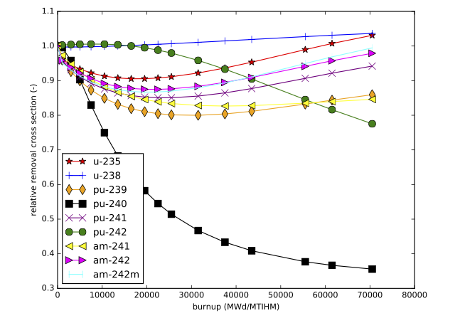
Fig. 5.1.2 Relative removal cross section as a function of burnup for key actinides (Westinghouse 17 \(\times\) 17 assembly with 5\% enrichment).
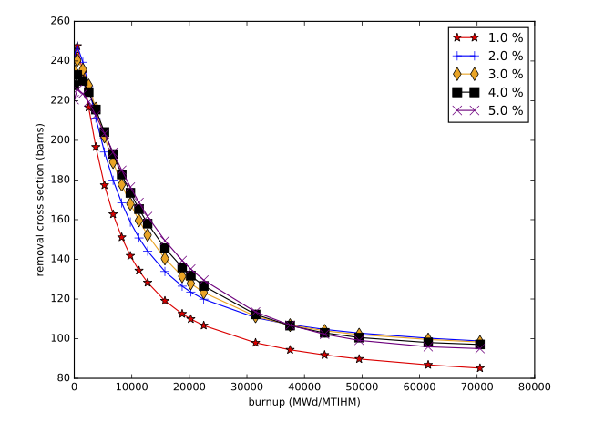
Fig. 5.1.3 240Pu-240 removal cross section as a function of burnup for various enrichments (GE 10 \(\times\) 10 assembly).
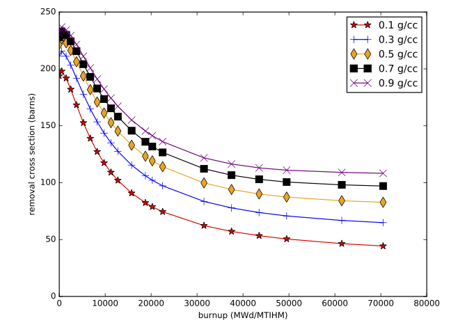
Fig. 5.1.4 240Pu removal cross section as a function of burnup for various moderator densities (GE 10 \(\times\) 10 assembly).
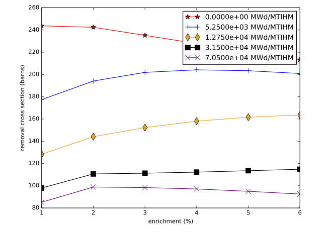
Fig. 5.1.5 240Pu removal cross section as a function of initial enrichment for various burnups (GE 10 \(\times\) 10 assembly).
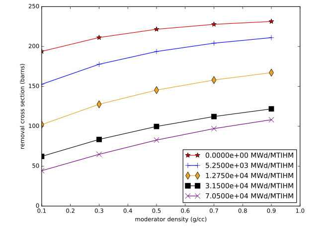
Fig. 5.1.6 240Pu removal cross section as a function of moderator density for various burnups (GE 10 \(\times\) 10 assembly).
Currently there are two interpolation methods: a Lagrangian based on low-order polynomials and a cubic spline with an optional monotonicity fix-up.
5.1.3.1.5.1. Lagrangian Interpolation
Lagrangian interpolation [ORIGEN-REFed68] seeks the unique n-1 order polynomial that will pass through n-points of the function and then interpolating to the desired point by evaluating the polynomial,
where \(x_{i}\) and \(y_{i}\) are the known x- and y-values in the neighborhood of the desired x-value x, with n the number of data points/order of Lagrangian interpolation. Note that Lagrangian interpolation is by definition local, involving only points in the neighborhood of the desired value. Global alternatives such as Hermite cubic splines use the entire data set to construct the interpolants. Common interpolation methods based on polynomials can have difficulty with data that vary quickly and have uneven x-spacing, as is expected with transition data. Polynomials tend to produce unphysical oscillations in these cases. In cases with very small y-values (~10-10), oscillations of the interpolant can produce negative interpolated values.
5.1.3.1.5.2. Cubic Spline Interpolation
Cubic spline interpolation has been observed to produce fewer, lower frequency oscillations. Oscillations can be effectively eliminated by enforcing monotonicity on the interpolation: that is, additional max maxima or minima are not introduced by the interpolant between known values of the function. Monotonic cubic splines [ORIGEN-WA02] have shown particularly stable behavior and have been implemented as an interpolation option.
5.1.3.1.6. Sensitivity Coefficient Calcualtion
Sensitivity calculations in ORIGEN allow one to determine the change in a particular response to all nuclear data involved in the calculation, including decay constants, fission product yields, one-group cross sections, and branch ratios.
The sensitivity coefficient of response, \(R\), due to a change in parameter \(\alpha\) is defined as
where \(R_0\) and \(\alpha_0\) are the nominal values for the response and data, respectively. The response is allowed the following form:
where \(N_i(t^*)\) is the nuclide amount at a specific point in time, \(t^*\), and \(h_i\) is the so-called realization vector, and \(u_i\) is a user-provided multiplier that can be used to target certain nuclides.
The implementation follows [ORIGEN-Wil86] with a simplifying assumption that data variations do not induce flux spectrum or flux magnitude variations, resulting in the sensitivity expression
where transition matrix \(\mathbf{A}(t)\) is in practice given piecewise-constant in time and nuclide adjoint \(\vec{N}_k^*(t)\) is calculated by the following final value equation:
where \(\mathbf{A}^T\) is the transpose of the transition matrix and final condition is given by \(N_i^*(t^*)=h_i u_i\). The system is then solved backwards in time to \(t=0\). Note that only the CRAM solver kernel in ORIGEN can perform the adjoint calculation.