5.1.5. ORIGEN Module
The ORIGEN module drives depletion, decay, and activation calculations as described in Sect. 5.1.3.1, including the conversion of generated powers to fluxes described in Sect. 5.1.3.1.3, as well as alpha, beta, gamma, and neutron source calculations described in Sect. 5.1.3.1.4.
5.1.5.1. Key Features
This section briefly highlights some key features in ORIGEN and describes how they are used.
5.1.5.1.1. Nuclide Specification and ORIGEN Sub-libraries
The nuclide identifiers in ORIGEN are more flexible than those in other modules of SCALE and even within the ORIGEN family. Table 5.1.1 shows the possible ways to specify nuclides (and elements).
Identifier Form |
Comments |
Examples |
|
|---|---|---|---|
nuclide |
input id |
||
IZZZAAA
|
Standard numeric identifier with one optional digit of isomeric state, three digits of atomic number, three digit of mass number; elements have mass number of 000. |
235U |
92235 |
235mU |
1092235 |
||
135Xe |
54135 |
||
1H |
1001 |
||
10B |
5010 |
||
Fe |
54000 |
||
EAm
|
Standard symbolic identifier with element symbol followed by mass number, followed by optional metastable indicator; can include a dash between E and A (E-Am); case insensitive. |
235U |
u235 |
235mU |
u235m |
||
135Xe |
xe135 |
||
1H |
h1 |
||
10B |
b10 |
||
Fe |
fe |
One important aspect ORIGEN users must be aware of is that the ORIGEN library (f33) being used dictates the set of nuclides available in a calculation and that there may be more than one version of a nuclide in a library. The duplicates arise in large part from the need to analyze fission products separately. For example, a gadolinia-doped uranium oxide fuel with burnup will have some 155Gd from the initial gadolinia loading and some 155Gd generated as a fission product. Although these fuels physically behave the same way, it is sometimes important to be able to analyze them separately. These groups, versions, or categories are referred to as sublibraries because in an ORIGEN library, they appear almost like three separate, smaller ORIGEN libraries. The three libraries are for
naturally occurring, light nuclides, sometimes called “light elements” or “activation products,”
actinides and their reaction and decay products, and
fission products.
Called “sublibs” for short, they are identified by a number or 2-character specifier:
light nuclides with “LT” or 1,
actinides with “AC” or 2, and
fission products with “FP” or 3.
The production of fission products from actinides (2/AC3/FP) is the only type of transition in a typical ORIGEN library that spans sublibs. The sublib is optional in a nuclide specification and is indicated in parentheses after the identifier-IZZZAAA(S), EAm(S). If the sublib for a nuclide/element is not provided, it is guessed in the following manner:
If the nuclide is in fact an element, then it is placed in sublib=1/LT.
If the atomic number Z < 26, an attempt is made to place it in sublib=1/LT.
Otherwise (Z \(\geq\) 26 or attempt fails), sublibs are searched in reverse order, from 3/FP, 2/AC, and then 1/LT.
The third rule, which is to search sublibs in reverse order, correctly handles spent reactor fuel, a common and important scenario. The other two conditions can be interpreted as exceptions. The first exception correctly handles activation scenarios where it is most convenient to specify the initial elemental constituents. The second exception handles light nuclides that could not be real fission products, as fission products have Z \(\geq\) 26 by definition. The byproducts 1H, 2H, 3H, 3He, and 4He actually exist in all sublibs, but FP and AC byproducts have a reduced set of transitions compared to the LT version, which has full decay and activation chains. Thus when a user specifies one of the byproduct nuclides as input, it is best to associate it to the LT version.
5.1.5.1.2. Physical Units in Calculations
A variety of units can be used in the input and specified for the output of an ORIGEN calculation. The input allows for initial concentrations in
grams,
moles (or gram-atoms),
number density in atoms/barn-cm, and
curies.
Time may be expressed in seconds, minutes, hours, days, years, or a user-defined unit. Irradiation may be expressed in terms of neutron flux (n/cm2-s) or power (W). The allowed units for output include those for input, as well as the following decay quantities:
total decay heat power (W),
gamma decay heat power (W),
airborne toxicity (m3) required to dilute activities to the Radiation Concentration Guide (RCG) limit for air,
ingestion toxicity (m3) required to dilute activities to the RCG limit for water, and
alpha, beta, neutron, photon sources (particles/s or MeV/s).
Table 5.1.2 summarizes the available units in ORIGEN. During irradiation cases, the following can also be returned:
absorption rates (absorptions/s),
fission rates (fissions/s), and
infinite neutron multiplication constant, k\(_{\infty}\).
Unit name |
Description |
Input |
Output |
|
|---|---|---|---|---|
(irrad.) |
(decay) |
|||
GRAMS |
Mass in grams |
* |
* |
* |
MOLES or GRAM-ATOMS |
Number in moles (or legcy equivalent of gram-atoms) |
* |
* |
* |
ATOMS-PER-BARN-CM |
Density in atoms/barn-cm (10-24 cm/barn \(\times\) density in atoms/ cm3); requires volume input |
* |
* |
* |
CURIES |
Activity in curies |
* |
* |
* |
BECQUERELS |
Activity in becquerels |
* |
* |
* |
ATOMS_PPM |
Atom fractions x 106 |
* |
* |
|
WEIGHT_PPM |
Weight fractions x 106 |
* |
* |
|
WATTS |
Total decay heat in watts |
* |
||
G-WATTS |
Total decay heat from photons in watts |
* |
||
M3_AIR |
Radiotoxicity m3 for for inhalation |
* |
||
M3_WATER |
Radiotoxicity in m3 for ingestion |
* |
||
5.1.5.1.3. Saving Results
ORIGEN can save any results (isotopics and source spectra) in a special ORIGEN binary concentrations file (f71). The file is a simple sequence of solutions, and new results are simply appended on to the end of an existing file. Note that no matter how initial isotopics are entered or what units are asked for in the output file, the ORIGEN f71 contains moles (gram-atoms) of each isotope and an optional volume to permit unit conversions to number density (atoms/barn-cm). Isotopics for an ORIGEN calculation can be initialized from any position on this file in an ORIGEN calculation. The f71 can also be read by OPUS to perform various post-processing tasks.
5.1.5.2. Input Description
ORIGEN uses the SCALE Object Notation (SON) language for its input, although it can also read FIDO-based input for backwards compatibility with SCALE 6.1 [ORIGEN-ORN11]. The basic structure of an ORIGEN input is shown in Example 5.1.1.
 'SCALE comment
 =origen

 % ORIGEN comment %

 bounds{ … }
 solver{ … }
 options{ … }

 case(A){
     time=[31 365] % days
     …
 }

 case(B){
    …
 }
 …
 % more cases?

 end
The ORIGEN input is hierarchical, containing four levels, where level 0 is the “root” level, allowed between “=origen” and “end.” The complete set of keywords is shown in Table 5.1.3, with arrays denoted with “=[]” and blocks with “{}”. Referring to the overview in Example 5.1.1, at the root level, there is a “solver” block for changing solver options, a “bounds” block for entering the energy boundaries for various particle emissions, and an “options” block for altering the miscellaneous global options. These blocks may only appear once. The remainder of the input is a sequence of “case” blocks (in the above examples there are two cases with identifiers “A” and “B”), which each case is executed in order, with each case possibly depending on one or more of the previous cases.
Level 0 |
Level 1 |
Level 2 |
Level 3 |
|---|---|---|---|
|
title |
||
time{} |
start t=[] units custom_name custom_length |
||
lib{} |
file pos |
||
flux=[] |
|||
power=[] |
|||
print{} |
cutoff_step absfrac_step absfrac_sublib rel_cutoff cutoffs fisrate kinf |
||
nuc{} ele{} |
sublibs=[] total units=[] |
||
neutron{} |
summary spectra detailed |
||
gamma{} |
summary spectra principal_step unbinned_warning principal_cutoff |
||
alpha{} |
summary spectra |
||
beta{} |
summary spectra principal_step principal_cutoff |
||
mat{} |
iso=[] feed=[] units previous volume blend=[] |
||
load{} |
file pos |
||
save{} |
steps=[] file time_offset time_units |
||
neutron{} |
alphan_medium alphan_bins alphan_cutoff alphan_step |
||
gamma{} |
sublib adjust_for_missing conserve_line_energy split_near_boundary continuum immediate brem_medium spont |
||
alpha{} |
|||
beta{} |
sublib |
||
|
nuclide{} |
type=NAMED_SET |
list |
decay{} |
coeff_update[] allow_zero |
||
type=ENDF_DECAY |
resource |
||
type=ORIGEN_LIBRARY |
file |
||
neutron{} |
coeff_update[] allow_zero reaction_resource fp_yield_resource |
||
type= ENDF_ENERGY_ DEPENDENT |
spectrum{} xs_update{} |
||
|
alpha=[] beta=[] gamma=[] neutron=[] |
||
|
type |
||
opt{} |
terms maxp abstol reltol calc_type order substeps |
||
|
print_xs digits fixed_fission_energy |
||
The percent sign (%) is the comment character inside the ORIGEN sequence, between “=origen” and “end.” The % is a very flexible comment that may be placed almost anywhere in the input and continues until the end of the line. Outside the ORIGEN sequence, the SCALE comment character of a single quote ‘ at the beginning of a line must be used. Arrays in SON begin with “[” and end with “]” and support the following special shortcuts inherited from FIDO. Note that the interpolation shortcuts (I and L) insert values between two specified values so that there will be N+2 values in the final expanded array section.
Shortcut |
Format |
Examples shortcutexpansion |
|---|---|---|
Repeat (R) |
NRX |
3r1e141e14 1e14 1e14 6r3 3 3 3 3 3 3 |
Linear interpolation (I) |
NI X Y |
3i 5 1 5 4 3 2 1 9i 0.0 1.0 0.0 0.1 0.2 0.3 0.4 0.5 0.6 0.7 0.8 0.9 1.0 |
Log interpolation (L) |
NL X Y |
3l 1 5 5l 1e-9 1e-3 1e-9 1e-8 1e-7 1e-6 1e-5 1e-4 1e-3 |
As an alternative to manually creating an ORIGEN input file via a text editor, the user may use the SCALE graphical user interface (GUI) Fulcrum to create ORIGEN input files. Advantages to using Fulcrum include syntax highlighting, autocomplete, immediate feedback when input is incorrect, and one-click running of calculations.
5.1.5.2.1. Calculation Case (case)
A single ORIGEN sequence may contain an unlimited number of case blocks. Each case block is processed in order and can represent either an independent calculation or continuation of a previous case. The complete contents of a single case block are shown in Table 5.1.1.
 case(ID){
    title="my title"

     lib{ … }
     mat{ … }
     time{ … }
     flux{ … } % or power{ … }

     print{ … }
     save{ … }

     alpha{ … }
     beta{ … }
     gamma{ … }
     neutron{ … }
 }
The most important three components are the lib, mat, and time/power/flux inputs:
an ORIGEN library and the transition matrix data set on it to use (lib),
initial amounts of nuclides (mat), and
a power or flux history (time/power or time/flux).
The case identifier and case title string (shown as ID and title=”my title” in Example 5.1.2) are echoed in the output file and can be a convenient way to differential cases. Both are optional, with the ID defaulting to the case index, with “1” for the first case, “2” for the second, etc. The “print” and “save” blocks represent two ways to analyze the output from a calculation. The “print” block prints tables directly to the output file, and the “save” block saves the solution in a special ORIGEN binary concentration file (f71), e.g., for later post-processing. Finally, the “alpha,” “beta,” “gamma,” and “neutron” blocks control the emission source calculations for alpha, beta, gamma, and neutron particles, respectively. The remaining subsections will describe the input for each of these blocks.
5.1.5.2.2. Transition Matrix Specification (lib)
The transition matrix to use in a case is controlled by the “lib” shown in Example 5.1.3.
 lib{
     file="origen.f33"  % ORIGEN library filename
     pos=1              % data set position on library
 }
A “lib” must be present in the first case with a defined ORIGEN library file. The default position is “pos=1”. The “lib” may be omitted in subsequent cases, and if so, the previous case’s “lib” is used. The position refers to the set of transition coefficients (transition matrix A) to load. To load another position on the same library file, the “lib” block with “pos=X” can be used to load position X. When ARP generates an ORIGEN library, it will contain a set of transition coefficients for each requested burnup. When COUPLE generates an ORIGEN library, it will contain a single position. For decay calculations, file=”end7dec” can be used to load a decay-only library.
5.1.5.2.3. Material Specification (mat)
The initial isotopics for a case a controlled by the “mat” shown in Example 5.1.4. Note that the material specification has a few different variants, with only one allowed to specify the material in a given case.
 % from iso
 mat{
     iso=[ u235=1.0 u238=9.0 ] %id(sublib)=amount
     units=GRAMS               %units in iso array
 }

 % from iso with number density input
 mat{
     iso=[ u235=1e-2 u238=1e-1 ] %id(sublib)=amount
     units=ATOMS-PER-BARN-CM     %units in iso array
     volume=200                  %cm^3
 }

 % from position on f71 file
 mat{
     load{ file="origen.f71" pos=11 }
 }

 % from previous case (previous=LAST is default)
 mat{
     previous=4 %step index from previous case
 }
In the first variant in Example 5.1.4, the isotopic distribution “iso” is used with “units.” The “iso” array contains a sequence of “id=amount” pairs, where “id” is a nuclide identifier in the format described in Sect. 5.1.5.1.1, and the units of the amount are given by the “units” keyword, one of the unit names listed in the third column of Table 5.1.2. Default units are MOLES.
In the second variant, the number density (ATOMS-PER-BARN-CM) is specified which requires an additional specification of the “volume” in cm3. Internally, the number density will be converted to MOLES using that volume. For any type of units specified internally for calculations, isotopics are always converted to MOLES and then reconverted to the output units required.
In the third variant, the isotopics are loaded from a specific position on the f71 file. Note that the position index starts at one (not zero) and because the f71 is always appended to, it may contain multiple materials, cases, timelines, etc. In the fourth and final variant, the isotopics are loaded from end of step 4 from the previous case (“previous=4”). The index zero (e.g., “previous=0”) corresponds to the initial isotopics of the previous case. The keyword “LAST” may be used to load the isotopics from the end of the last step, “previous=LAST”. This is the default behavior, used when a “mat” block is not present.
There are two additional special material specifications shown in Example 5.1.5: (1) with a feed rate term, \(\overrightarrow{S}(t)\) in Eq. (5.1.4), or (2) the blend array. The feed specified is in the units specified per second and constant for the entire case. It is possible to perform a calculation with feed but with zero initial isotopics by specifying “iso=0”. Feed can be negative, however, the calculation becomes undefined and will abort when the number of atoms of any nuclide becomes negative.
The blend array allows a fraction of each result from the previous cases to be loaded. The identifier is the case name, or the index of the case if a case name is not provided and the fraction is the atom fraction. The step index for the isotopics can be specified in parentheses. For example, B(2)=0.9 indicates that 90% of the case(B) isotopics should be taken at the end of step 2. The default step index is the final step for the case. Only one blend is allowed in an ORIGEN input (between “=origen” and “end”). Multiple blends currently requires saving isotopics to an f71 file and reloading in a subsequent calculation.
 % with feed array
 mat{
     % units for iso and feed
     units=GRAMS

     % material is natural sodium
     iso=[na=1.0e6]
     % with feed array, set initial isotopics of zero
     %iso=0

     % continuous feed of U-235 at 1 kg/day
     % converted to grams/second
     feed=[u235=0.01157]
 }

 % with blend array (only one allowed in an input)
 case(A){ … }
 case(B){ … }
 case{
     …
     mat{
         % case ID(step index)=fraction of atoms
         blend[ A=0.1 B(2)=0.9 ]
     }
 }
5.1.5.2.4. Operating History (power, flux, time)
The operating history is specified using “time,” “power,” and “flux,” with examples shown in Example 5.1.6. For decay cases, only the “time” array in units of days is required. For irradiation cases, either “power” or “flux” may be provided. When flux is used, it is the step-wise flux \(\Phi_{n}\ \left( \frac{n}{cm^{2}s} \right)\) appearing directly in the depletion equations of Eq. (5.1.4). When power is used, it is the total step-average power– \(P_{n}\ (MW)\) –converted to step-wise average flux using Eq. (5.1.40). With irradiation cases using flux or power, the same number of entries must be specified on the time and flux/power array. The start time corresponding to the initial conditions is not included in the array of time values. Additionally, the time specification allows time units (including a custom unit) and a start time in which the block form of “time” must be used “time{…}.”
% simple decay case (two steps 0 unicode::U+2192 1 and 31 unicode::U+2192 65 days)
time = [ 31 365 ]

% flux irradiation (decay if flux=0)
time = [ 31   365  396 ]
flux = [ 2e14 1e14 0 ]

% power irradiation (decay if power=0)
time = [ 31 365 396 ]
power= [ 50 45  0 ] %50 MW, 45 MW, then decay

% changing units using time block
time{
    t = [ 5 15 300 ]
    units = HOURS
    % available units:
    % SECONDS, MINUTES, HOURS, DAYS, YEARS, CUSTOM
}

% custom units
time{
    t = [ 1 2 3 ]
    units = CUSTOM
    custom_name = "MONTH"
    custom_length = 2678400 %seconds per "MONTH"
}

% 10-step detailed power history
time=[   5  10 20 100 300 400 405 500 800 1000]
power=[ 20  41 43  42  37  33  16 14.5 28.5 26]
To illustrate some aspects of specifying a power history, refer to Fig. 5.1.7, where the black line (“actual power”) shows a piecewise linear power history that is translated to a possible step-wise constant power history shown by the red line (“step-wise constant power”), with input shown in Example 5.1.6 labeled “10-step detailed power history”. The secondary (right) y-axis shows the step-wise flux, calculated from the step-wise power via the predictor-corrector approach of Eq. (5.1.40). The dependence of the power-to-flux conversion on the actual material composition is shown in the comparison of flux results for an initial composition with 6% fissile 235U (blue dotted line) versus 2% fissile 235U (purple dashed line). The flux at the beginning of the irradiation is a factor of 3 higher with the 2% fissile case, due to approximately a factor of 3 lower fissile content. With time, fissile plutonium build-up closes the gap to a factor of 1.5.
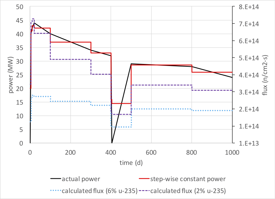
Fig. 5.1.7 Example of ORIGEN operating history and power-to-flux conversion.
% first case
case{
    mat{ … }
    time=[ 1 10 25 50]
    flux=[ 4r1e14 ]
}
% continuation case (time zero is 50 days)
case{
    time{
        units=YEARS
        %without start, times must continue > 50 days
        %t=[50/365.+0.1 50/365.+0.3 … ]
        %with start=0, times given assume start at zero
        start=0
        t=[0.1 0.3 0.9 2.7]
    }
}
By default, subsequent cases that continue operations on a material, continue the timeline of that material. Using “start=0” is convenient when switching time unitsfrom irradiation in days to decay time in years, for example. Otherwise, the final time must be converted to years.
5.1.5.2.5. Printing Options (print)
The “print” command is one of the most complex inputs, with options to set printing cutoffs and control the concentrations returned, broken down by nuclides and elements and emission sources for gamma, neutron, alpha, and beta particles. Additionally, there are options to print fission rates, absorption rates, and the ratio of fission rate to absorption rate. Each case is allowed a print block.
5.1.5.2.5.1. Inventories by nuclide and element
The options for printing nuclides and elements are shown in Example 5.1.8. The print block allows the “nuc” block and “ele” block for printing nuclide and element results, respectively.
% print each nuclide (total across all sublibs) in grams
print{
    nuc{ total=yes units=GRAMS }
}

% print each element (total across all sublibs)
% in moles, grams, and curies with cutoffs of 1%
print{
    ele{ total=yes units=[MOLES GRAMS CURIES] }
    cutoffs[ ALL=1.0 ]
}

% print decay heat and mass (by element)
% of fission products and actinides only
print{
    ele{ sublibs=[AC FP] units=[GRAMS WATTS] }
}

% change cutoff to absolute curies by element,
% in step of interest (7), but print GRAMS
print{
    cutoff_step = 7 % default -1 for average
    rel_cutoff = no % default is yes for cutoff in percent
    % only print above 1e-3 curies
    cutoffs[ CURIES=1e-3 ]   % default is 1e-6 percent
    nuc{
     total=yes
     units=GRAMS
    }
}
Inside the “nuc” or “ele” blocks, there are three possible entries:
a “sublibs” array (a list from LT, AC, FP, ALL),
a “total” (yes or no), and
a “units” array (see column 1 of Table 5.1.2 for possible units).
The “total” is whether to sum over all “sublibs,” i.e., if Gd-155 occurs in both LT and FP sublibs, then the total will be the sum of the two. It is possible to have “sublibs=[LT AC FP] total=yes,” which results in four output tables, one for each of the sublibs and one for the total. The specification of “sublibs=ALL” is the same as “sublibs=[LT AC FP].”
Three parameters set the cutoff for printing a nuclide or element:
“cutoff_step” sets the index on which to base the cutoff (default -1 means use an average over all steps),
“rel_cutoff” determines whether to treat the cutoff as a percent of the total (default/yes) or an absolute amount (no), and
the “cutoffs” array allows one to specify the cutoff for each unit in Table 5.1.2 as a sequence of “unit=cutoff” pairs.
5.1.5.2.5.2. Radiological Emissions (alpha, beta, gamma, neutron)
The emission printing options are controlled by the “alpha,” “beta,” “gamma,” and “neutron” emission blocks inside a “print” block (examples shown in Example 5.1.9).
print{
    % default neutron options
    neutron{
     summary=yes
     spectra=no
     detailed=no
    }

    % default gamma options
    gamma{
     summary=yes
     spectra=no
     principal_step=NONE  %step index to calculate
                          %(NONE to suppress)
     principal_cutoff=2   %principal emitter cutoff
                          %in percent
     unbinned_warning=no  %print warning
                          %when line not binned
    }

    % default alpha options
    alpha{
     summary=yes
     spectra=no
    }

    % default beta options
    beta{
     summary=yes
     spectra=no
     principal_step=NONE  %step index to calculate
                          %principal (NONE to suppress)
     principal_cutoff=2   %principal emitter cutoff
                          %in percent
    }
} %end print
Neutron print options
The “neutron” print options are
“summary” (yes/no) controls the printing of a source strength summary,
“spectra” (yes/no) controls the printing of the spectra (energy group-wise), and
“detailed” (yes/no) controls the printing of extra details about the neutron calculation.
The “gamma” print options are
“summary” (yes/no) controls the printing of a source strength summary and
“spectra” (yes/no) controls the printing of the spectra (energy group-wise).
Gamma print options
The gamma print allows a special output of the principal emitters in each energy group, controlled by setting the “principal_step” keyword to a specific step index in the case, with the “principal_cutoff” keyword used to set the minimum percent of the total a nuclide must have to be considered a principal emitter. For the gamma print there is a warning that can be enabled with “unbinned_warning=yes” if some gamma lines fall outside the user group structure and thus are not included.
Alpha print options
The “alpha” print options are
“summary” (yes/no) controls the printing of a source strength summary and
“spectra” (yes/no) controls the printing of the spectra (energy group-wise).
Beta print options
The “beta” print options are
“summary” (yes/no) controls the printing of a source strength summary and
“spectra” (yes/no) controls the printing of the spectra (energy group-wise).
The beta print also allows a special output of the principal emitters by setting the “principal_step” keyword to a specific step index in the case, with the “principal_cutoff” keyword used to set the minimum percent of the total a nuclide must have to be considered a principal emitter.
The special printing options are shown in Example 5.1.10.
% defaults special printing options
print{
    absfrac_sublib = ALL %print absorption fractions for
                         %a specific sublib (LT,AC,FP)
                         %or ALL sublibs (DEFAULT)

    absfrac_step = 7  %if absfrac active, step to print
                      % default is last step

    fisrate = NONE    %print fission rates (default NONE)
                      %absolute (ABS) or relative (REL)

    kinf = no         %print fission/absorption (yes/no)
}
5.1.5.2.6. Saving Results (save)
Saving the results to an ORIGEN binary file (f71) is requested with the “save” block, which specifies both the name of the file and the step indices to save, as shown in Example 5.1.11. The default for the filename is “file=ft71f001” and default for the steps is the special “steps=ALL” which saves all isotopics and spectra as a shortcut to having to specify “steps=[0 1 2 3 … LAST]”. The step index “0” corresponds to the initial isotopics and the step index “LAST” may be used as a shortcut for the last case index. There is a special rule for copying f71 files from SCALE’s temporary/working directory. If the file name “ft71f001” exists in the directory when SCALE finishes, it is copied to the user’s “${OUTDIR}” as “${BASENAME}.f71”, e.g. if my.inp produces “ft71f001” in the temporary/working directory then it will be copied to the same location as the main output file (“my.out”) as “my.f71”. Note that f71 files are always appended to by ORIGEN. To save with the defaults, the shortcut “save=yes” is provided. The default is “save=no”.
case{
    mat{ … }
    time=[ 1 10 100 1000 ] % 4 steps to 1000 days
    save{
          file="short.f71"   % file name
          steps=[0 2 4]      % save initial (0) and isotopics
                                 % end-of-step 2 (10 days)
                                 % end-of-step 4 (1000 days)
    }

    save{
          file="ft71f001"   % file name (DEFAULT)
          steps=ALL         % save ALL steps (DEFAULT)
    }
    save=yes              % equivalent to the above

    save{
          file="last.f71"   % file name
          steps=[LAST]      % save only last (LAST=4 here)
          time_offset=1000  % write time - time_offset
          time_units=DAYS   % units of time_offset
    }
}
In order to change the time values written to the f71 file, use “time_offset=T0” which will write the current cumulative time minus T0 to the file. The “time_offset” is convenient, for example, when time since discharge is desired instead of the absolute, cumulative time. The “time_units” entry specifies the units of the “time_offset”, with the same units available in the “time” block. The default is “time_units=DAYS”.
5.1.5.2.7. Decay Emission Calculations (alpha, beta, gamma, neutron)
A decay emission calculation is initiated with the appropriate block inside the calculation “case.” The group structure for any emission spectra result is determined by the energy bounds provided as described in Sect. 5.1.3.1.4. Each type of emission calculation is activated by the existence of a calculation block named “alpha”, “beta”, “gamma”, or “neutron” for those respective types of calculations. Alternatively, to turn on an emission calculation with defaults, use “alpha=yes”, “beta=yes”, “gamma=yes”, or “neutron=yes” in a “case” block.
5.1.5.2.7.1. Neutron source calculation
The neutron calculation (Sect. 5.1.3.1.4.1) is activated by the “neutron” calculation block. All neutron calculation options are to control the \(\left(\alpha,n\right)\) calculation.
Three \(\left(\alpha,n\right)\) options can be indicated with the “alphan_medium”: a UO2 fuel matrix (alphan_medium=UO2), a borosilicate glass matrix (alphan_medium=BOROSILICATE), and the problem-dependent matrix defined by the user input compositions (alphan_medium=CASE). The numeric options 0, 1, and 2 are also valid for the UO2, BOROSILICATE, and CASE options, respectively. Note that the UO2 and borosilicate glass matrix options assume that the neutron source nuclides reside in these respective matrices, regardless of the actual composition of the material in the problem.
For oxide fuels, a significant neutron source can be produced from 17O \(\left(\alpha,n\right)\) and 18O \(\left(\alpha,n\right)\) reactions in the oxygen compounds of the fuel. For this reason, the UO2 matrix option (enabled by alphan_medium=UO2) is provided with natural isotopic distribution of 17O and 18O. This includes the impact of oxygen isotopes on the neutron source without having to include oxygen in the initial composition.
Another common use case is fuel storage in a borosilicate glass matrix
(enabled by alphan_medium=BOROSILICATE), listed in
Table 5.1.5 from [ORIGEN-DJPB86].
Elements with atomic number less than 17 have \(\left(\alpha,n\right)\)
yields.
Atomic number |
Element symbol |
Wt % |
Atom % |
|---|---|---|---|
3 |
Li |
2.18 |
6.296 |
5 |
B |
2.11 |
3.913 |
8 |
O |
46.4 |
58.138 |
9 |
F |
0.061 |
0.0644 |
11 |
Na |
7.65 |
6.671 |
12 |
Mg |
0.49 |
0.404 |
13 |
Al |
2.18 |
1.620 |
14 |
Si |
25.4 |
18.130 |
17 |
Cl |
0.049 |
0.0277 |
20 |
Ca |
1.08 |
0.540 |
25 |
Mn |
1.83 |
0.668 |
26 |
Fe |
8.61 |
3.091 |
28 |
Ni |
0.70 |
0.239 |
40 |
Zr |
0.88 |
0.193 |
82 |
Pb |
0.049 |
0.0047 |
Total |
99.669 |
100.000 |
|
In the last most rigorous option, the \(\left(\alpha,n\right)\) neutron source and spectra are calculated using the source, target, and constituents determined using the material compositions in the problem at a particular time, dictated by “alphan_step” in the “neutron” print options. For spent fuel neutron source calculations, there are a large number of potential source, target, and constituent nuclides in the \(\left(\alpha,n\right)\) calculation and in order to remove low-importance nuclides from the calculation, the “alphan_step” and “alphan_cutoff” parameters are used. Only those nuclides with an \(\alpha\)-decay activity exceeding the product of “alphan_cutoff” times the total \(\alpha\) activity are included as source nuclides in the \(\left(\alpha,n\right)\) neutron calculation. Additionally, only those nuclides with a constituent or target atom fraction less than “alphan_cutoff” are included unless the concentration is greater than 1 ppm, in which case it will be retained regardless of the cutoff. The “blend” array is particularly useful for creating a problem-dependent medium composed of fuel and another material.
case{
    …
    neutron{
          alphan_medium=CASE %0/UO2 for UO2
                                 %1/BOROSILICATE
                                 %  for Borosilicate glass
                                 %2/CASE for case-specific (DEFAULT)
          alphan_bins=200    %use 200 bins for
                                 %alpha slowing down calculation
          alphan_cutoff=0.0  %cutoff for alpha,n calculation
          alphan_step=LAST   %step index in this case
    }
    %alternatively, to enable neutron calculation with defaults
    %neutron=yes
}
5.1.5.2.7.2. Gamma source calculation
The gamma (photon) calculation described in Sect. 5.1.3.1.4.4 is activated with the “gamma” block, as shown in Example 5.1.13. The gamma block includes a host of options where the default should be appropriate in most cases.
The “sublib” option (default “ALL”) affects the sublibraries included in the gamma emission calculation. The “immediate” option (default “yes”) includes immediate gamma and x-rays.
The “spont” option (default “yes”) includes photons emitted during spontaneous fission and \(\left(\alpha,n\right)\).
The “continuum” option (default “yes”) enables mapping of continuum data stored artificially as lines to a continuum across the user-defined energy bins.
The following options may need to be modified in some scenarios.
The “brem_medium” option (default “UO2”) includes the photons emitted by beta particles as they slow down in a medium (Bremsstrahlung) in the gamma calculation. A problem-dependent medium is not available for “brem.” The only options are “NONE,” “H2O” (for Bremsstrahlung in water) and “UO2” (for uranium dioxide).
The “conserve_line_energy” option (default “no”) modifies the intensity of each gamma line within a group to conserve energy according to Ig = Ia Ea/Eg, where Ia is the original line intensity, Ea the original line energy and Eg is the group energy (simple midpoint energy). Note that this option modifies intensities and thus results in number of particles not being conserved.
The “adjust_for_missing” option (default “no”) accounts for the scenario where a nuclide has a known gamma decay mode with known recoverable energy release, but the spectral data do not exist in the available emission resource. If “adjust_for_missing=yes,” the entire spectrum is scaled up to include the missing energy. If the missing energy is more than 1% of the total, a warning is printed.
The “split_near_boundary” option (default “no”) enables a splitting of a line when it appears very close to a bin boundary. If “split=yes” and a photon line is within 3% of an interior energy boundary, then the intensity is split equally between the adjacent groups.
case{
    …
    gamma{
         sublib=ALL      %LT, FP, or AC - single sublib
                         %ALL - all sub-libraries
         brem_medium=UO2 %assume Bremsstrahlung in UO2
         continuum=yes   %expand continuum data stored as
                         %lines into proper continuua
         immediate=yes   %load lines for immediate gamma/x-rays
         spont=yes       %include photons from
                         %spontaneous fission
                         %and alpha,n reactions

         conserve_line_energy=no %conserve line energy instead
                                 %of line intensity
         adjust_for_missing=no   %adjust photon intensity
                                 %for energy of missing spectra
         split_near_boundary=no  %lines within 3% of a
                                 %group boundary are split
                                 %into two bins
    }
    %alternatively, to enable gamma calculation with defaults
    %gamma=yes
}
5.1.5.2.7.3. Alpha and beta source calculation
The alpha calculation (Sect. 5.1.3.1.4.2) has no options and the beta calculation (Sect. 5.1.3.1.4.3) only has a single option to choose the nuclide sublibraries included (see Example 5.1.14). Note that the alpha and beta calculations determine sources and do not include any slowing down physics for charged particles.
case{
    …
    alpha{
        %no options
    }
    %alternatively, to enable alpha calculation with defaults
    %alpha=yes

    beta{
       sublib=ALL  %LT, FP, or AC - single sublib
                   %ALL - all sub-libraries
    }
    %alternatively, to enable beta calculation with defaults
    %beta=yes
}
5.1.5.2.8. Processing Options (processing)
The processing options are contained inside the “processing” block (inside a “case”) and have two ways to modify the isotopics vector: the “removal” block and the “retained” array (see ::numref::fig-origen-processing-block). Both operate on elements instead of nuclides.
Each “removal” block specifies a list of elements and a rate of continuous removal in units (1/s). This removal is an artificial increase of the decay constant, from Eq. (5.1.4), and it can be used to model any continuous system of removal, such as filtration. Note that more than one removal block may be specified.
The “retained” array specifies a list of elements and the mole/atom fraction to be retained at the start of this case. Note that all unspecified elements become zero.
case{
    …
    processing{
        %rate is in 1/s
        removal{ rate=1e-2 ele=[H Xe Ar] }
        removal{ rate=1e-7 ele=[U Pu] }
        %id=frac
        retained=[ u=1.0 pu=0.5 ]
    }
}
5.1.5.2.9. Bounds Block
The “bounds” block appears outside all cases and is valid for the entire input, dictating the energy bins (i.e., groups) for emission spectra and source calculations (see Example 5.1.16). The array shortcuts-“L” for logarithmically spaced intervals and “I” for linearly-spaced intervals-can be particularly useful for specifying the bounds (see Table 5.1.4). The energy bounds are in units (eV) and can be given in increasing or decreasing order with the output convention of decreasing order. Additionally, neutron and gamma energy bounds can be read from a standard SCALE cross section library file by specifying the path to the file instead of the array bounds.
=origen
bounds{
    neutron=[1e6 1e3 1] %2-group with 1MeV, 1keV, 1eV
    gamma=[100L 1.0e7 1.0e-5] %101 logarithmically spaced bins
    alpha=[1e6 2e7] %high-energy bin between 1 and 20 MeV
    beta=[22I 1 100] %23 linear bins between 1 and 100 eV
    %read neutron bounds from SCALE multi-group library file
    %neutron="scale.rev04.xn252v7.1"
}
case{ … }
end
5.1.5.2.10. Solver Block
The solver block controls high-level solver options, the most important of which is the actual solver kernel used, either the default MATREX (Sect. 5.1.3.1.2.1, Example 5.1.17) or CRAM (Sect. 5.1.3.1.2.2, Example 5.1.18).
=origen
solver{
    type=MATREX    %(DEFAULT)
    opt{
        terms=21   %number of expansion terms (DEFAULT)
        maxp=100   %maximum number of short-lived precursors
                   % for a long-lived nuclide (DEFAULT)
        substeps=1 %number of time step divisions (DEFAULT)
    }
}
case{ … }
end
=origen
solver{
    type=CRAM
    opt{
        order=16   %order of the method (DEFAULT)
        substeps=1 %number time step divisions (DEFAULT)
    }
}
case{ … }
end
The MATREX kernel contains two parameters that are generally sufficient with the default values. The minimum number of “terms” is \(n_{terms} =21\), which overrides the heuristic in Eq. (5.1.20). Experience indicates that high flux levels (e.g., greater than 1016 n/cm2-s) may require more terms. The second parameter, “maxp,” is generally sufficient, describing the amount of storage available for the short-lived precursors of a long-lived isotope.
The CRAM kernel has a single parameter that impacts the numerical error: the “order.” Both the CRAM and MATREX solver include the “substeps” parameter that adds substeps to each user-defined time step. Testing the same input with a different number of substeps (e.g., “substeps=1,” “substeps=2,” “substeps=4”) can be a simple way to check that the time grid is sufficient.
5.1.5.2.11. Options Block
The “options” block contains miscellaneous global options that apply to all cases, as shown in Example 5.1.19. The “print_xs” option enables output of the transition matrix A used in each case, the “digits” option enables high-precision output when set to 6, and the “fixed_fission_energy” allows 200 MeV per fission to be used everywhere instead of the nuclide-dependent energy release being used by default.
=origen
options{
    print_xs=no             %print cross sections
    digits=4                %digits=6 is high-precision
    fixed_fission_energy=no %set to yes to use 200 MeV/fission
}
case{…}
end
5.1.5.2.12. Library Building Block build_lib
This block allows one to create an ORIGEN library within an ORIGEN input. The basic usage is to create a library, “A.f33” in the example below, and then use this library in a calculation.
=origen
build_lib("A.f33"){
  ...
}
case{
  lib{ file="A.f33" pos=1 }
  ...
}
end
The build_lib block is composed of three main sub-blocks:
nuclide{ ... }: nuclides to consider,decay{ ... }: decay data data to use, andneutron{ ... }: incident neutron data to use.
These blocks are designed to be extensible and will gain additional capabilities
in future versions. Note that the obiwan command-line utility
(see Sect. 5.2) is useful in the view mode to understand the
contents of your library file.
Note
Previously, this was the purpose of the COUPLE module, which is deprecated as of SCALE 6.3.
5.1.5.2.12.1. Nuclide Block build_lib/nuclide
The build_lib/nuclide block contains the information on which nuclides
to consider in the final library. One can read data from any source for any
nuclide, and this will be echoed in the output file; however, only the nuclides
defined here will be allowed in the final ORIGEN library. The default and
only options for the nuclide block are type=NAME_SET with the
nuclide set complete_v6.2, which is defined as the set of 2237 nuclides
(including sub-libraries) used in SCALE v6.2.
=origen
build_lib("A.f33"){
  nuclide{
    type=NAMED_SET
    list="complete_v6.2"
  }
  ...
}
...
end
Note
The entire build_lib/nuclide block will default to the above for
SCALE 6.3.
5.1.5.2.12.2. Decay Data Block build_lib/decay
The build_lib/decay block contains the fundamental decay data with which
to build the library. With this block, there are currently two options:
type=ORIGEN_LIBRARY, which loads decay data from an existing ORIGEN library specified with thefile=input.type=ENDF_DECAY`, which loads decay data from any supported decay resource using the ``resource=input—both ORIGEN card-image formats (legacy) and ENDF-formatted data.
Creating a basic ORIGEN decay library is now trivial.
=origen

build_lib("my_decay.f33") {
  nuclide {
    type=NAMED_SET
    list="complete_v6.2"
  }
  decay {
    type=ENDF_DECAY
    resource="${DATA}/origen_data/origen.rev03.decay.data"
  }
}

end
Note
All ORIGEN inputs that expect paths (e.g., resource) now expand SCALE
environment variables such as ${DATA} and ${INPDIR}, which can
be very convenient as it avoids having to use =shell to copy needed
files to the working directory.
Updating specific decay coefficients
One final input is available in the decay block, coeff_update, which
allows one to specify specific decay channels and yields to update.
The specific format is
coeff_update[
  parent "channel(yield)" value
  ...
]
where
parentis the parent nuclide id or name,channelis the numeric identifier for the decay channel,yield(optional) is the isomeric state of the daughter (e.g., 0 or 1), andvalueis the actual value for the decay constant or yield.
As an example, the following input changes the alpha decay data for 238U, after it loads the nominal data from the decay resource.
=origen

build_lib("end7dec.f33") {
  nuclide {
    type=NAMED_SET
    list="complete_v6.2"
  }
  decay {
    type=ENDF_DECAY
    resource="${DATA}/origen_data/origen.rev03.decay.data"
    coeff_update [
        u238  "5"        1e-12   % alpha decay (5) in 1/s
        u238  "5(0)"     0.9000  % alpha decay (5) yield to residual in ground (0)
        u238  "5(1)"     0.1000  % alpha decay (5) yield to residual in 1st meta (1)
    ]
  }
}

end
The decay channel identifiers are shown in the following table.
Channel Identifier |
Decay Mode |
|---|---|
1 |
Gamma |
2 |
Beta Minus |
3 |
Beta Plus |
4 |
Isomeric Transition |
5 |
Alpha |
6 |
Neutron |
7 |
Spontaneous Fission |
8 |
Proton |
9 |
Unknown |
Note that a decay channel can be composed of multiple, chained modes. For
example, a \(2\beta_- + n\) decay channel would have identifier 226.
Notes on Spontaneous Fission
Spontaneous fission has been historically accounted for in ORIGEN in an
unexpected way. The spontaneous fission mode is included in the overall
decay constant but the individual fission product yields are not modeled
by default. With the coeff_update block it is possible to add
spontaneous fission, but one must be careful: no matter what the input
is, the yields will be renormalized to sum to 2.0, as in a physically meaningful
fissioning system. For this reason, it may be beneficial to introduce a
fake target for most spontaneous fissions if one’s interest
is just in modeling a few key fission products.
With spontaneous fission, the “yield” identifier is the target fission product nuclide identifier in IZZZAAA format.
For example, consider this fake spontaneous fission data which uses 12C as a fake target nuclide.
=origen

build_lib("end7dec.f33") {
  nuclide {
    type=NAMED_SET
    list="complete_v6.2"
  }
  decay {
    type=ENDF_DECAY
    resource="${DATA}/origen_data/origen.rev03.decay.data"
    coeff_update [
        cf252 "7(6012)"  1.80000 % spontaneous fission (7) to fake target C-12 because yields must normalize to 2.0
        cf252 "7(54135)" 0.1600  % 8% of FPs are Xe135
        cf252 "7(53135)" 0.0400  % 2% of FPs are  I135
    ]
  }
}
5.1.5.2.12.3. Neutron Data Block build_lib/neutron
The build_lib/neutron block contains the fundamental incident neutron
data on which to build the library. With this block, there is currently only
a single option, type=ENDF_ENERGY_DEPENDENT, which allows the following
inputs.
reaction_resource, a path to the reaction resource to load, sometimes referred to as a “JEFF” library because the current data originates from JEFF/3.0-A.fp_yield_resource, a path to the fission product yield resource, which may be an ORIGEN card-image format (legacy) or ENDF-formatted data.
With these resources loaded, one must add a flux spectrum to determine energy-integrated values for all reactions and fission product yields.
For example, the following input creates a complete library (decay and neutron data) using the 56-group reaction resource with a constant flux spectrum, 1.0 for all groups.
=origen

build_lib("B.f33") {

  nuclide {
    type=NAMED_SET
    list="complete_v6.2"
  }

  decay {
    type=ENDF_DECAY
    resource="${DATA}/origen_data/origen.rev03.decay.data"
  }

  neutron(1) {
    type=ENDF_ENERGY_DEPENDENT
    reaction_resource="${DATA}/origen.rev01.jeff56g"
    fp_yield_resource="${DATA}/origen_data/origen.rev05.yield.data"

    spectrum {
      type=MULTIGROUP
      flux=[56R 1.0]
    }

  }
}

end
The spectrum block currently has two types.
type=MULTIGROUPto provide afluxin the same group structure as the reaction resource. Future versions will have additional flexibility to provide the flux spectrum in any group structure.type=AMPX_LIBRARYto provide the spectrum from an AMPX library, which requires bothfileandmixtureinputs, which specify the AMPX library file and the mixture number, respectively.
The following input is an example of loading a spectrum directly from an AMPX multigroup library.
=origen

build_lib("B.f33") {

  nuclide {
    type=NAMED_SET
    list="complete_v6.2"
  }

  decay {
    type=ENDF_DECAY
    resource="${DATA}/origen_data/origen.rev03.decay.data"
  }

  neutron(1) {
    type=ENDF_ENERGY_DEPENDENT
    reaction_resource="${DATA}/origen.rev01.jeff56g"
    fp_yield_resource="${DATA}/origen_data/origen.rev05.yield.data"

    spectrum {
      type=AMPX_LIBRARY
      file="sysin.microWorkLib_0.f44"
      mixture=1
    }
  }
}

end
Note that this assumes that sysin.microWorkLib_0.f44 exists in the temporary
working directory and contains mixture 1 data.
The neutron/spectrum is all that is needed to collapse to one-group reactions
and interpolate fission product yields. However, this will neglect important cross
section self-shielding effects. In general, self-shielding
is very important for thermal systems and where there is a significant amount of
a strong resonance absorber which will depress the flux spectrum and implicitly
reduce the cross section in that energy range. This is the main purpose of the
xs_update block which allows one to read multi-group cross sections from
a file, collapse those with the flux spectrum from the spectrum block, and
use those preferentially over any “unshielded” data from the reaction resource.
In the following input, the AMPX library is used in both the spectrum and
cross section update. Note the spectrum and xs_update blocks are
identical for the AMPX_LIBRARY type.
=origen

build_lib("B.f33") {

  nuclide {
    type=NAMED_SET
    list="complete_v6.2"
  }

  decay {
    type=ENDF_DECAY
    resource="${DATA}/origen_data/origen.rev03.decay.data"
  }

  neutron(1) {
    type=ENDF_ENERGY_DEPENDENT
    reaction_resource="${DATA}/origen.rev01.jeff56g"
    fp_yield_resource="${DATA}/origen_data/origen.rev05.yield.data"

    spectrum {
      type=AMPX_LIBRARY
      file="sysin.microWorkLib_0.f44"
      mixture=1
    }
    xs_update {
      type=AMPX_LIBRARY
      file="sysin.microWorkLib_0.f44"
      mixture=1
    }
  }
}

end
The final optional component of the neutron block is the coeff_update
list, which can directly set the values of transition coefficients both in
terms of cross section channels and daughter yields.
The specific format is
coeff_update[
  parent "channel(yield)" value
  ...
]
where
parentis the parent nuclide id or name,channelis the numeric identifier for the reaction channel, commonly called “MT” numbers (see Sect. 10.1.3.1 for details),yield(optional) is the isomeric state of the daughter (e.g., 0 or 1) or the actual nuclide identifier in the case of fission (channel=18), andvalueis the actual value for the one-group reaction cross section or yield.
For example, consider this code excerpt which modifies the fraction of 241Am \((n,\gamma)\) which results in 242mAm and 242Am. Note that an appropriate energy-integrated value was determined from the reaction resource and the flux spectrum, and this update overwrites that value.
=origen

build_lib("B.f33") {

  ...

  neutron(1) {
    ...
    coeff_update[
      am241 "102(1)" 0.7 % 70% of n,gamma go to Am-242m
      am241 "102(0)" 0.3 % 30% of n,gamma go to Am-242
    ]

  }
}

end
Note
Yields are always renormalized to sum to 1.0 as a final step before creating the ORIGEN library, except for fission (channel=18), which is renormalized to sum to 2.0. In the above example, if you provided only one yield (e.g., the 0.70 to 242mAm), then the final yields will be renormalized to sum to 1.0, and your final yield will not be 0.70.
5.1.5.2.12.4. Data Cutoffs
The legacy COUPLE library building (see Sect. 5.1.9.4) included
an internal cutoff for decay constants of approximately 2.0E-26 and for cross
sections of approximately 1e-20 barns. It makes sense to have cutoffs from the
perspective of computational efficiency; however, one issue with cutoffs is that as the system
evolves, there may be reactions below the cutoff (and not included)
that then should be included. Although we could allow for this flexibility
eventually, the ability to change the nuclides and transitions considered
during a depletion calculation is not allowed, and it must be fixed from the
beginning. For this reason, allow_zero options exist in both the decay
and neutron blocks to change this legacy cutoff to zero.
See example Example 5.1.32 for details.
5.1.5.2.13. Sensitivity Calculation Block sens
The sensitivity calculation described in Sect. 5.1.3.1.6 is activated with the “sens” block.
Consider the following complete case, which irradiates 1 gram of 238U
using the transition.def ORIGEN library file. This is a useful library
to use for testing but has assumed a uniform flux spectrum and thus will not be
accurate for any real scenario.
=origen
solver{
  type=cram
}

case(A){
  lib{ file="transition.def" }
  mat{ iso=[ u238=1.0 ] units=GRAMS }
  time=[ 20I 3 1000]
  flux=[ 22R 1e14 ]
  save=yes
}

sens{
  case=A
  response{ iso=[pu239=1.0] type=NUCLIDE step=LAST }
  threshold=1e-4

  dp_verify{
    nrank=3
    nrank_pert=1.001
  }
}

end
The components of the sens input are as follows.
case: the name of the case to consider the forward calculation. Note that the default name for the first case is “1”, second case is “2”, etc.response: a block that defines the type of response (see below for details).iso: is a user multiplier for each nuclide in the responsestep: the step index at which the relative change in the response will be analyzed.
threshold: the minimum sensitivity coefficient to print in the output file.dp_verify: a block that defines “direct perturbation” cases to verify the sensitivities. Direct perturbations can point out useful issues with time steps too large for the forward/adjoint calculations or a response that is particularly difficult to integrate (e.g., rapidly changing amount over a time step). Even though the forward and adjoint solutions will be accurate on the time steps, the integration of the forward solution multiplied by the adjoint over all steps assumes a simple trapezoid rule and could be inaccurate.nranknumber of direct perturbations to perform per category of sensitivity (currently 6) for each sensitivity coefficient which exceeds thethreshold.nrank_pertperturbation factor to assume for the direct perturbation verification. For example, “1.01” would indicate to multiply the data of interest by 1.01 (i.e., increase by 1%).
5.1.5.2.13.1. Response definitions
Internally, the response type handles setting response realization vector \(h_i\) and user multiplier \(u_i\) from Eq. (5.1.56).
For type=NUCLIDE, \(h_i=1\). The default user-specified multiplier is \(u_i=0\).
Any entries in the iso array of the response block will modify \(u_i\).
This will typically be a single value of 1.0 for a single nuclide of interest, e.g.
iso=[ pu239=1.0 ] to calculate the sensitivity of final Pu-239 inventory to all data.
5.1.5.2.13.2. Sensitivity output tables
The main output of the sensitivity calculation is sent to the .out file and is shown below.
--------------------------------------------------------------------------
Sensitivity Calculation Summary (#1/1)
--------------------------------------------------------------------------

Forward calculation case                           = A
Target step (from case)                            = 22
Corresponding target time (seconds)                = 86400000.000000
Sensitivity coefficient report threshold           = 0.000100
Response type                                      = nuclide
Number of direct perturbation checks per group     = 3
Direct perturbation factor (multiplier)            = 1.001000
Adjoint concentration file                         = adjoint.sens1-adj.f71

----------------------------------------------------------------------
Total Decay Loss Sensitivity
----------------------------------------------------------------------
-------------------------------------------------------------------------------------
| Nuclide ID | Adjoint Sens. Coeff. | Direct Sens. Coeff. | Direct F71 File         |
-------------------------------------------------------------------------------------
|      93239 |          7.83906e-02 |         1.10034e-03 |  adjoint.sens1-dps1.f71 |
|      94241 |          4.77040e-04 |         4.77023e-04 |  adjoint.sens1-dps2.f71 |
|      96242 |          2.49246e-04 |         2.51713e-04 |  adjoint.sens1-dps3.f71 |
-------------------------------------------------------------------------------------

----------------------------------------------------------------------
Decay Loss Sensitivity
----------------------------------------------------------------------
--------------------------------------------------------------------------------------------------------
| Nuclide ID |    Decay Mode   | Adjoint Sens. Coeff. | Direct Sens. Coeff. | Direct F71 File          |
--------------------------------------------------------------------------------------------------------
|      93239 |           beta- |          7.83906e-02 |         1.10034e-03 |   adjoint.sens1-dps4.f71 |
|      94241 |           beta- |          4.77029e-04 |         4.77013e-04 |   adjoint.sens1-dps5.f71 |
|      96242 |           alpha |          2.49246e-04 |         2.51713e-04 |   adjoint.sens1-dps6.f71 |
--------------------------------------------------------------------------------------------------------

----------------------------------------------------------------------
Decay Yield Sensitivity
----------------------------------------------------------------------
No sensitivities exceed the threshold.

----------------------------------------------------------------------
Total Reaction Loss Sensitivity
----------------------------------------------------------------------
-------------------------------------------------------------------------------------
| Nuclide ID | Adjoint Sens. Coeff. | Direct Sens. Coeff. | Direct F71 File         |
-------------------------------------------------------------------------------------
|      94239 |         -9.92411e-01 |        -9.89541e-01 |  adjoint.sens1-dps7.f71 |
|      92238 |          6.58620e-01 |         7.32985e-01 |  adjoint.sens1-dps8.f71 |
|      93239 |         -1.80910e-03 |        -1.95421e-03 |  adjoint.sens1-dps9.f71 |
|      94238 |          4.60255e-04 |                   - |                       - |
|      95241 |          2.95686e-04 |                   - |                       - |
|      94241 |         -2.14775e-04 |                   - |                       - |
-------------------------------------------------------------------------------------

----------------------------------------------------------------------
Reaction Loss Sensitivity
----------------------------------------------------------------------
-------------------------------------------------------------------------------------------------------
| Nuclide ID |     Reaction    | Adjoint Sens. Coeff. | Direct Sens. Coeff. | Direct F71 File         |
-------------------------------------------------------------------------------------------------------
|      92238 |         n,gamma |          6.59038e-01 |         7.33404e-01 | adjoint.sens1-dps10.f71 |
|      94239 |         fission |         -6.55423e-01 |        -6.53213e-01 | adjoint.sens1-dps11.f71 |
|      94239 |         n,gamma |         -3.37762e-01 |        -3.36715e-01 | adjoint.sens1-dps12.f71 |
|      93239 |         n,gamma |         -1.80585e-03 |                   - |                       - |
|      94238 |         n,gamma |          4.63905e-04 |                   - |                       - |
|      92238 |         fission |         -3.71955e-04 |                   - |                       - |
|      95241 |         n,gamma |          2.96838e-04 |                   - |                       - |
|      94241 |         fission |         -1.57067e-04 |                   - |                       - |
-------------------------------------------------------------------------------------------------------

----------------------------------------------------------------------
Reaction Yield Sensitivity
----------------------------------------------------------------------
No sensitivities exceed the threshold.
The six groups of sensitivities are as follows.
Total decay loss sensitivity – the relative change in response per change in a nuclide’s total decay constant.
Decay loss sensitivity – the relative change in response per change in specific decay channels (e.g., \(\alpha\)-decay).
Decay yield sensitivity – the relative change in response per change in a decay yield—for example, the fraction of \(\gamma\)-decays that result in the ground state daughter versus a metastable daughter.
Total reaction loss sensitivity – the relative change in response per change in a nuclide’s total loss cross section.
Reaction loss sensitivity – the relative change in response per change in specific reaction channels (e.g. \((n,\gamma)\)).
Reaction yield sensitivity – the relative change in response per change in a reaction yield, (e.g., fission product yields).
Note that for each group, three direct perturbation calculations are performed
because nrank=3. Thus, if an ORIGEN forward calculation only takes a second,
and the adjoint calculation takes approximately the same, in this case there
are 12 additional forward calculations performed. If there were any yield
sensitivities, the number could be as high as 18. For this reason, small
nrank is recommended.
According to the sensitivity output, the dominant sensitivities are related
to reactions on 238U and 239Pu, which makes sense. The reaction loss
sensitivity table shows eight reactions that exceeded the sensitivity coefficient
threshold of 1e-4. It is interesting to note that some comparisons of the
adjoint sensitivity versus the direct sensitivity are very close, whereas the
238U \((n,\gamma)\) has an adjoint sensitivity of 0.66 and a direct of
0.73. This gap may decrease if the time steps for the forward calculations
in case “A” are reduced; however, it may also simply be a non-linearity.
The adjoint solution utilized here is first-order perturbation theory, whereas
the direct perturbation may capture additional orders of variation if the
perturbation applied (nrank_pert) is “large.” In this particular case,
reducing the perturbation factor to 1.0001 had no effect, but adding an
additional 20 time steps resulted in a closer adjoint value of 0.70 compared
to an unchanged direct value of 0.73.
5.1.5.2.13.3. Sensitivity output files
A number of f71 files are produced as a result of the sensitivity calculation.
${BASENAME}-sens<i>-adj.f71contains the adjoint solution for the<i>-th sensitivity calculation.${BASENAME}-sens<i>-dps<k>.f71contains the<k>-th direct perturbation solution for the<i>-th sensitivity calculation. Note the “Direct F71 File” column in the table indicates which one corresponds to which perturbation.