5.4. ORIGAMI: A Code for Computing Assembly Isotopics with ORIGEN

ORIGAMI computes detailed isotopic compositions for light water reactor assemblies containing UO₂ fuel by using the ORIGEN transmutation code with pre-generated ORIGEN libraries, for a specified assembly power distribution. The fuel may be modeled using either lumped or pinwise representations with the option of including axial zones. In either case, ORIGAMI performs ORIGEN burnup calculations for each of the specified power regions to obtain the spatial distribution of isotopes in the burned fuel. Multiple cycles with varying burn-times and downtimes may be used. ORIGAMI produces several types of output files, including one containing stacked ORIGEN binary output data (“ft71 file”) for each depletion zone; files with nuclide concentrations at the last time-step for each axial depletion region, in the format of SCALE standard composition input data or as MCNP material cards; a file containing the axial decay heat at the final time-step; and gamma and neutron radiation source spectra.

5.4.1. Acknowledgments

ORIGAMI is based on the PinDeplete code developed by Steve Skutnik and also includes techniques taken from the Orella code written by Ian Gauld (retired). Support for development of ORIGAMI was provided by the U.S. Department of Energy, Office of Nuclear Energy, Nuclear Fuels Storage and Transportation Planning Project.

5.4.2. Introduction

ORIGAMI (ORIGEN Assembly Isotopics) provides the capability to perform isotopic depletion and decay calculations for a light water reactor fuel assembly model using one or more ORIGEN calculations. The assembly may be modeled using either lumped or pinwise representations with the option of including axial zones. ORIGAMI automates the performance of ORIGEN depletion calculations for each region and thus simulates zero-, one-, two-, and three -dimensional (0D, 1D, 2D, and 3D) modeling of a fuel assembly. Multiple cycles with different specific powers and exposure and decay times may be treated, and the power distribution is described in terms of fractional pin powers in the XY plane and axial distributions along the Z axis, which define the burnup regions for the ORIGEN computations. ORIGAMI allows for easy and flexible material composition specification through the standard SCALE mixture processor for composition input, the same as in TRITON (see XSPROC chapter). While ORIGAMI cannot presently treat axially non-uniform lattice features (e.g. axially varying enrichment or the partial-length rods found in many boiling water reactor designs) within a single input, these problems can still be easily modeled by splitting the problem across sequential ORIGAMI input cases residing on the same file.

The ORIGEN calculations performed by ORIGAMI use the methodology originally established for the SCALE sequence ORIGEN-ARP (see the ARP section). This approach provides an efficient mechanism to perform stand-alone reactor depletion calculations using pre-generated ORIGEN libraries which contain self-shielded, collapsed one-group cross sections as a function of selected independent variables, such as burnup, enrichment, and moderator density, for different reactor systems. Typically the data in these libraries are obtained from 2D, multigroup lattice transport calculations (e.g., TRITON) coupled with depletion calculations for burnup. The library cross sections may be flux-weighted over the lattice to obtain data representative of the entire homogenized assembly for lumped depletion; or alternatively, it is also possible to generate multiple ORIGEN libraries corresponding to individual or groups of pins within the lattice for multi-pin depletion. The burnup-dependent ORIGEN libraries are analogous to the parameterized cross section data produced by lattice physics codes for reactor core simulators, except that data for many more nuclides and reactions are included to allow ORIGEN to compute detailed isotopics for more than 2200 nuclides.

ORIGAMI extends the capabilities previously provided by ORIGEN-ARP to perform a suite of ORIGEN calculations in order to represent the isotopic distribution of fuel within an assembly in more detail. The pre-generated ORIGEN libraries provided with SCALE tabulate the assembly-average one-group cross sections, in order to accurately reproduce assembly-average isotopics. When performing pin-by-pin calculations in ORIGAMI, users can increase the fidelity with respect to proximity to features such as assembly edges, water holes, burnable poison rods, etc. by creating and employing zone-specific libraries for different pins. By specifying the individual library assignments for each pin, users can capture these local spectrum changes in the ORIGAMI calculation through the use of one-group libraries based on these local conditions. Currently, the specification of individual libraries is limited to pin-level specification only (i.e., the same library is used for all axial zones corresponding to a pin for 3D cases) with an allowed axial moderator density distribution and radial and axial power distributions.

ORIGAMI can produce the following output files in addition to the standard ORIGEN output for each depletion zone:

isotopics in ORIGEN binary concentration (ft71) files

in each depletion zone at times specified by the options block, ft71 key

in each axial zone (summed over all pins at a particular axial level) at the final time;

nuclide concentrations by axial zone, written as a SCALE “standard composition block” that can be used directly as input for SCALE transport codes such as the KENO Monte Carlo criticality code;

axially-dependent decay heat source for input to a thermal analysis code such as COBRA, so that the temperature distribution within a storage cask can be computed;

nuclide concentrations for each axial zone, given in the format of MCNP material cards;

space-dependent radiation source energy spectra and magnitudes in a simple text file.

ORIGAMI is tightly integrated with the SCALE Graphical User Interface, Fulcrum. Using Fulcrum and the “UO2 express form (configurable)”, one can create a simple UO₂ assembly depletion case in seconds (see Fig. 5.4.1). Finally, ORIGAMI has the ability to perform the depletion/decay calculations for each zone in parallel using the MPI (Message Passing Interface), however this requires a special SCALE installation built with MPI in order to do so [ORIGAMISHDLG13].

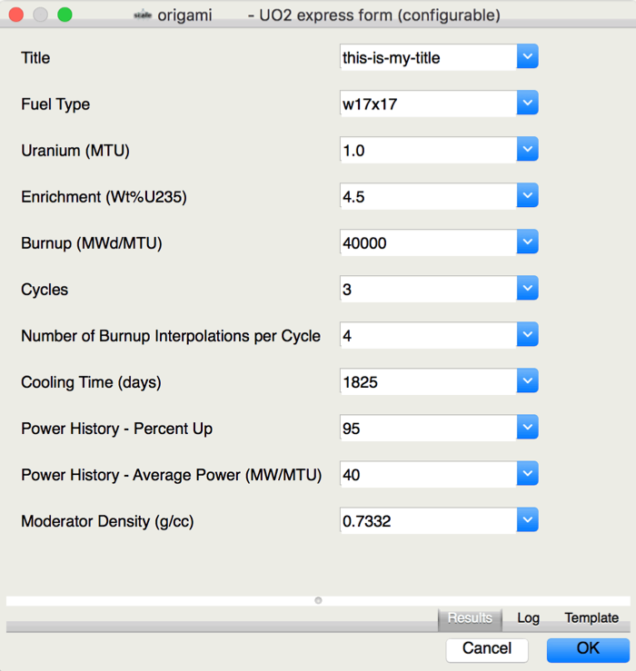
Fig. 5.4.1 Fulcrum UO₂ express form for creating ORIGAMI input.

5.4.3. Computational Methods

5.4.3.1. ORIGAMI assembly model

The basic model for ORIGAMI is a fuel assembly, which may be modeled in several ways with varying degrees of complexity. The most primitive model represents the assembly materials as a single mass lump that is depleted using the value of the specific power input in the power-history block. In this case, a single ORIGEN calculation is performed to obtain isotopics representing the entire assembly. This 0D model is equivalent to the conventional ORIGEN-ARP procedure. A more detailed model applies an input axial power profile to the (radially) lumped assembly materials. This lumped axial depletion model produces a 1D axially varying burnup distribution, but no allowance is made for variations in the relative pin powers within the assembly. Thus, if the axial power distribution is defined by N_Z axial zones, ORIGEN calculations are performed for N_Z different depletion regions. The 1D axial depletion model has been found to be adequate for most criticality and decay heat analysis of spent fuel assemblies [ORIGAMIRGlW12]. Note that both the 0D and 1D modes are fully consistent with the 2D TRITON calculations used to generate ORIGEN reactor libraries distributed with SCALE, in that these modes employ spatially-homogenized cross-sections to represent assembly-averaged flux and cross-sections. For 2D and 3D depletion models (wherein individual pin-specific libraries may optionally be specified), the user is advised that the ORIGEN reactor data libraries distributed with SCALE are representative of an assembly axial plane as a whole; in as much, the user is advised to generate their own zone-specific libraries (i.e., based on individual material zones) within TRITON if they wish to capture regional neutronic effects within the assembly (such as proximity to water holes, burnable absorbers, etc.)

By specifying a radial pin-power map, a 2D or 3D calculation may be performed. Currently the axial and radial power shapes are fixed for the entire calculation but do still result in a fully 3D isotopic distribution [ORIGAMISGRT12, ORIGAMISHDLG13]. If there are N_P pins in the assembly and each has N_Z axial zones, ORIGAMI will perform ORIGEN calculations for N_P $\times$ N_Z depletion regions. For example, an assembly with a 17 $\times$ 17 array with 264 fuel pins and N_Z = 24 axial zones requires 6336 independent ORIGEN calculations. For these types of simulations, the parallel mode with MPI is highly recommended.

5.4.3.2. Definition of initial composition

The initial mass in metric tons of heavy metal is M_mtu, set by the input parameter mtu. The default value of mtu is equal to 1.0, so that by default the ORIGEN calculations are performed on the basis of “per metric ton of heavy metal”. Given that the sum over all zones must have the total heavy metal content (M_mtu), one arrives at zone-wise heavy metal masses of:

(5.4.1)\[M_{xy,z} = \dfrac{M_{\text{mtu}}} { \sum \limits_{z = 1}^{N_{z}}{ f_{z} } \sum \limits_{xy = 1}^{N_{P}}{ m_{xy}} } \cdot f_{z} \cdot m_{xy}\]

where the relative amount of heavy metal in each radial position, :m_xy, is calculated from the mixture specification; fractional axial height, f_z, from the zone specification; and N_P and N_Z are the total number of fuel pins and axial zones, respectively. Note that some pin locations in the assembly may not contain fuel, and these are not included in the value of N_P. The fractional axial height is given

$f_z = \frac{\Delta Z }{Z_{\text{tot}}}$ is the fraction of the active fuel height occupied by axial zone Z $\Delta Z$ is the length of axial zone

Z_tot is the total length of the active fuel.

Whenever an axial zone mesh is input (with array meshz), the value of f_Z is computed from the values of the zone boundaries (see input description in Sect. 5.4.4.6). If an axial mesh array is not input, the axial zones are assumed to be uniformly distributed. In this case, the axial zones all have the same height, so that $f=\frac{1}{N_Z}$, where N_Z is the number of uniform axial zones in the assembly.

The uranium mass in a single axial zone for all N_P fuel pins in the assembly (M_z) is thus:

(5.4.2)\[M_Z = N_P \times M_{XY, Z} = M_{\text{mtu}} \times f_Z\]

In addition to the fuel mixture in an assembly, non-fuel materials (e.g., structural materials) may also be present. These materials contribute to the overall power production due to the energy produced by neutron capture reactions.. For a given value of the total assembly power, this reduces the power from the fuel mass and thus may slightly alter the fuel burnup and isotopics. In addition, activation of non-fuel materials produces additional radiation source terms in the spent fuel, which contribute to the decay heat and activity. Therefore ORIGAMI provides an option for including the non-fuel elements in the input array, nonfuel. The units of the non-fuel element masses are kg per MTU, and the materials are distributed uniformly within all fuel depletion zones. Note that the input non-fuel materials should not include oxygen in UO₂ if UO₂ is specified as the fuel material, as oxygen is already included in proportion to the uranium mass basis. Finally, because ORIGAMI accesses the StdComp library, any SCALE StdComp composition, e.g. “zirc4” for reactor cladding material Zircaloy-4, may be used in either structural or fuel materials.

5.4.3.3. Restart cases

ORIGAMI also allows the initial nuclide concentrations to be obtained from a previously produced ORIGEN binary output file. A restart case is indicated by setting restart=yes in the parameter array. The restart file has the name assembly_restart.f71 and must be copied (or linked) to the SCALE temporary directory used for calculations. The restart file is normally obtained from an earlier ORIGAMI calculation, which always produces an ORIGEN restart file named $OUTBASENAME.assm.f71, where ${OUTBASENAME} is an output prefix defined by the name of the input file and any user-specified prefix with the prefix key. Generally the restart file from ORIGAMI contains stacked concentrations, corresponding to each axial zone and then a final entry for the lumped assembly concentrations; hence, the initial composition for a restart case varies with axial zone, unlike the case for fresh fuel. ORIGAMI does not currently allow pin-dependent restart calculations. A restart case may be useful for performing decay-only calculations of spent fuel inventory, using the burned fuel composition previously computed for the assembly exposure during reactor operation. For decay-only cases, a value for the input parameter nz must be input in order to indicate the number of axial depletion regions in the previous burnup calculation.

5.4.3.4. Definition of power distribution

The radial power distribution is defined by the XY fractional pin powers in the input array pxy, and the axial fractional powers in the input array pz. The input values in arrays pxy and pz are normalized to unity by the code. The fractional power for a fuel pin “XY” is designated here to be r_XY, with the normalization $\sum_{XY = 1}^{N_{P}}r_{XY}$. Similarly the fractional axial power for an axial zone Z is a_Z, which is normalized to $\sum_{Z = 1}^{N_{Z}}a_{Z}$. The shapes of both the radial XY and axial Z distributions must be obtained prior to the ORIGAMI calculation, either from neutron transport calculations or experimental measurements. The input distributions remain constant during the ORIGEN burn calculations for all cycles; but in reality, the power distributions may vary with time—for example, the initial axial power distribution tends to flatten after a period of burnup since the higher power zones deplete the fuel faster. For this reason it is strongly recommended to use the relative burnup distribution (at final discharge) rather than the relative power density distribution for the input values. The burnup shape corresponds to the shape of the time-averaged flux distribution during the exposure period. This ensures that the final burnup distribution matches the desired shape.

Note

When comparing depletion calculations to an equivalent case from TRITON/NEWT or TRITON/KENO, it is important to note the difference between the total system power (which will include small contributions from the recoverable energy from non-fission capture reactions by the moderator and any structural materials) with the fuel power (used for the fuel depletion calculation). Because of the small contributions to the total system power from non-fuel regions, the fuel power will likely be smaller than the total system power, as specified in the burn block.

Thus, users wishing to compare the results of an ORIGAMI calculation to an equivalent TRITON calculation should ensure that that they are using the equivalent fuel mixture power from TRITON in ORIGAMI (and not the total system power); see Sect. 3.1.5.4.4 for further details.

For a given cycle, the assembly-specific power P^(SP) is equal to the value of input variable power, read in the power-history block (see Sect. 5.4.4.4). The assembly-specific power has units of megawatts per MTU (MW/MTU). Therefore, the total power produced by the fuel assembly is:

(5.4.3)\[P_{\text{tot}} = P_{A}^{\left( \text{SP} \right) } \cdot M_{\text{mtu}}\]

where P_tot is the assembly total power, and $P_{A}^{\left( \text{SP} \right)}$ is the specific power for the assembly, read from input.

The absolute power (MW) in fuel pin “XY” is:

(5.4.4)\[P_{P} = P_{\text{tot}} \cdot r_{xy} = P_{A}^{\left( \text{SP} \right)} \cdot M_{\text{mtu}} \cdot r_{xy}\]

and the power produced in axial zone Z of this fuel pin XY is:

(5.4.5)\[P_{XY,Z} = P_{\text{tot}} \cdot r_{xy} \cdot a_{Z} = P_{A}^{\left( \text{SP} \right)} \cdot M_{\text{mtu}} \cdot r_{xy} \cdot a_{Z}\]

The absolute power produced in a single axial zone Z for all pins is:

(5.4.6)\[P_{Z} = \sum_{XY = 1}^{N_{P}}{P_{XY,Z} = P_{\text{tot}} \times a_{Z} = P_{A}^{\left( \text{SP} \right)} \times M_{\text{mtu}} \times a_{Z}}\]

The ORIGEN depletion calculations are performed with the absolute powers defined in Eq. (5.4.4) and Eq. (5.4.6) for each depletion region in the 2D/3D pin-wise or 0D/1D axial depletion models, respectively. However, cross sections in the ORIGEN libraries are parameterized as a function of burnup, which depends on the specific power rather than absolute power for a given depletion region. The specific power (MW/MTU) in axial zone Z of pin XY is equal to:

(5.4.7)\[P_{XY,Z}^{(SP)} = \frac{P_{XY,Z}}{M_{XY,Z}}\]

Substituting Eq. (5.4.1) and Eq. (5.4.5) into Eq. (5.4.7) gives:

(5.4.8)\[P_{XY,Z}^{(SP)} = \frac{P_{A}^{(SP)} \cdot r_{\text{xy}} \cdot a_{Z} \cdot N_{P}}{f_{Z}}\]

In a similar manner, it can be shown that the specific power for all fuel pins in axial plane Z is:

(5.4.9)\[P_{Z}^{(SP)} = \frac{P_{A}^{(SP)} \cdot a_{Z}}{f_{Z}}\]

ORIGAMI permits two modes for user-specified power distributions along the axial and radial meshes: absolute fractions (i.e., where powers along the axial mesh points are expressed as fractions of the total assembly power in MW) and relative normalization (i.e., in which specific powers— in MW/MTU — of axial zones are expressed as a relative modifiers of the assembly specific powers input in the power history block). Relative power shape modifiers assume that the specific powers expressed in the power history block represent the average assembly specific power(s) thus, ORIGAMI will convert these factors into axial & pin power fractions — i.e., the factors r_xy and a_z found in Eq. (5.4.4) and Eq. (5.4.6) used to calculate the absolute pin power and axial zone power, respectively. The conversion from relative specific power modifiers to absolute power fractions is accomplished through the following normalization procedure Eq. (5.4.10):

(5.4.10)\[\left( a_{Z} \right)_{i} = \frac{ \left( R_{Z} \right)_{i} \cdot M_{\text{MTU}} \cdot \left( \frac{\Delta Z}{Z_{\text{tot}}} \right)_{i}} {\sum{\left( R_{Z} \right)_{i} \cdot M_{\text{MTU}} \cdot \left( \frac{\Delta Z}{Z_{\text{tot}}} \right)_{i}}} = \frac{\left( R_{Z} \right)_{i} \cdot \left( \frac{\Delta Z}{Z_{\text{tot}}} \right)_{i}}{\sum{\left( R_{Z} \right)_{i} \cdot \left( \frac{\Delta Z}{Z_{\text{tot}}} \right)_{i}}}\]

where $\left( a_{Z} \right)_{i}$ is the axial power fraction for axial zone i and $\left( R_{Z} \right)_{i}$ is the relative axial zone specific power modifier for axial zone i. Obviously, for a uniformly-spaced axial mesh, the conversion from relative specific powers (using relative power modifiers) is precisely the same as that for absolute fractional axial zone powers; i.e., the relative power modifiers simply become axial power fractions by virtue of the fact that the term $\left( \frac{\Delta Z}{Z_{\text{tot}}} \right)_{i}$ becomes a constant, thereby reducing Eq. (5.4.10) back to a direct calculation of the fractional axial power based on a relative power modifier following normalization.

Because it is assumed that the assembly mass is uniformly distributed across the pins, it can similarly be shown that the use of relative power modifiers for the XY pin map $\left( r_{XY} \right)_{i}$ will always produce the same result as using pre-normalized absolute fractional powers in the pin map, i.e. Eq. (5.4.11):

(5.4.11)\[\left( r_{XY} \right)_{i} = \frac{\left( R_{XY} \right)_{i} \cdot \frac{M_{\text{MTU}}}{N_{P}}}{\sum_{}^{}{\left( R_{XY} \right)_{i} \cdot \frac{M_{\text{MTU}}}{N_{P}}}} = \frac{\left( R_{XY} \right)_{i}}{\sum_{}^{}\left( R_{XY} \right)_{i}}\]

This option is provided as the relnorm option in the parameters block (discussed further in Sect. 5.4.4.2). The motivation for providing an alternative normalization for axial power shape factors is twofold. First, it is generally assumed that information on the axial power shape is obtained from axial measurements relative to an assembly-average value (i.e., axial gamma scans to determine the burnup profile based upon the gross gamma intensity or isotopic ratios of burnup indicators such as ¹³⁴Cs / ¹³⁷Cs, etc.). Therefore, by using the relative normalization option (i.e., treating axial power shape factors as relative modifiers of the assembly specific power), users can directly input shape factors obtained from techniques such as non-destructive analysis (NDA) fuel measurements into ORIGAMI to model assembly isotopic distributions.

The second motivation for the relative normalization option comes from potential problems that can arise if treating axial power shape factors as absolute fractional powers (relnorm=no) in conjunction with non-uniform axial mesh spacing defined by the user in the z array (see Sect. 5.4.4.7 for details).

Important

If using the relnorm=no option, the fractional axial powers must be consistent with the axial mesh sizes defined or else incorrect zone-specific powers will be calculated in Eq. (5.4.9), possibly causing the calculated burnup values to be out of the library range.

Users are thus strongly cautioned when using absolute fractional axial powers (relnorm=no) to ensure proper consistency between the axial power fractions and the axial mesh sizes.

For this reason, relative power shape factor normalization is turned on by default (relnorm=yes).

5.4.3.5. Computation of neutron and gamma energy spectra

ORIGAMI includes an option to generate multi-group neutron and gamma source spectra due to radioactive decay, for each depletion zone. Multi-group values are calculated by binning the discrete line and continuum spectra produced by radioactive decay and nuclear reactions into arbitrary energy group structures defined by user input. Whenever neutron energy group boundaries are input in array ngrp, neutron source spectra due to spontaneous fission, delayed neutron emission, and $\left( \alpha, n\right)$ reactions are calculated.

Similarly, gamma source spectra are computed if gamma energy group bounds are input in array ggrp. The gamma source includes photons produced by all types of radioactive decays, and also may include bremsstrahlung radiation produced by beta interactions. Input options can specify the type of nuclides included in the source term (i.e., light elements, actinides, fission products, or all nuclides), and the materials used for $\left( \alpha,n \right)$ reactions and bremsstrahlung production. If source spectra are calculated, the values are always included in the ORIGEN output ft71 binary file; and optionally the source spectra may also be output in a text file. The source text file only includes the average over all pins for each axial zone, while the ft71 file includes sources for all pins and axial zones.

The source spectra output by ORIGAMI are calculated in ORIGEN using the expression outlined in Eq. (5.4.12):

(5.4.12)\[S_{\text{Z.g}}^{(p)} = \sum_{i = 1}^{\text{itot}}{Y_{i,g}^{(p)}\lambda_{i} \frac{M_{Z}^{(i)}}{A^{(i)}} \cdot N_{A}}\]

where

$S_{\text{Z.g}}^{(p)}$ = source spectrum (p/s) in energy group g for particles of type p and axial zone Z;

$Y_{i,g}^{(p)}$ = number of particles of type p emitted per decay of nuclide i; with energy in group g;

$M_{Z}^{(i)}$ = mass (g) of nuclide i in axial zone Z, obtained from ORIGEN calculation;

N_A = Avogadro’s number (number atoms of nuclide i per mole);

A⁽ⁱ⁾ = mass (g) of 1 mole of nuclide i;

$\lambda_i$ = decay constant (s^-1) for nuclide i,

itot = total number of nuclides in burned fuel.

More details on the ORIGEN calculation of the source spectra can be found in the ORIGEN section (Sect. 5.1.5.2.5.2) of the SCALE documentation.

5.4.4. ORIGAMI Input Description

ORIGAMI uses free-form, keyword-driven input with the SCALE Object Notation (SON) syntax also used for ORIGEN input, and is described in more detail there. The general outline of ORIGAMI input is as follows.

Case Identifier

Options

Fuel Composition

Power-History

Source-Options

Output-Print Options

Input Data

The above input data may be entered in any order. Data blocks and parameters which are not needed, or for which default values are desired, can be omitted. Example 5.4.1 provides a template containing all of the ORIGAMI input data blocks and arrays, with example values assigned. Note that much of the information shown in the template is optional, and typically is not needed for many cases. The following subsections provide a more detailed description of the input.

Example 5.4.1 Template for ORIGAMI input data

 =origami
 % Case identifier information
   title= 'input template example'
   prefix= example
   asmid=1
 % Parameter options
   options{
     pitch= 19.718
     mtu= 0.4
     decayheat=yes
     fracnf=0.08
     nburn=15
     ndecay=12
     temper=300.0
     stdcomp=yes
     restart=no
     interp=spline
     output=cycle
     ft71=all
   }
 % Array containing ORIGEN library names
   libs=[ ce14x14 ce16x16 ]
 % Fuel Composition
   fuelcomp{
     uox(fuel1){ enrich=3.21 }
     uox(fuel2){ enrich=3.50 }
     uox(fuel3){ enrich=2.80 }
     mix(1){ comps[ fuel1=98.2 Gd2O3=1.8 ] }
     mix(2){ comps[ fuel2=100 ] }
     mix(3){ comps[ fuel2=97.5 Gd2O3=2.5 ] }
     mix(4){ comps[ fuel3=96.9 Gd2O3=3.1 ] }
   }
 % Map ORIGEN library names to XY pin layout
   libmap=[ 1 2
            2 1 ]
 % Map individual compositions XY pin layout
   compmap=[ 1 2
             3 4 ]
 % XY relative power distribution (code renormalizes to unity)
   pxy=[ 0.2 0.3
         0.4 0.5 ]
 % Z-axial relative power distribution (code renormalizes to unity)
   pz=[ 0.6 0.4 ]
 % Axial interval boundaries (for MTU mass distribution & plotting)
   meshz=[ 0.0 15.0 30.0 ]
 % Non-fuel nuclides distributed within fuel material
   nonfuel=[ cr=3.366 mn=0.1525 fe=6.309 co=0.0302
             ni=2.366 zr=516.3 sn=8.412 gd=2.860 ]
 % Axial variation of moderator density fraction
   modz=[ 0.73 0.715 ]
 % Irradiation/decay information
   hist[
     cycle{ power=35.0 burn=200.0 nlib=7 down=50.0 }
   ]
 % Optional neutron/gamma source information
   ggrp=[ 10.0e6 2.0e6 1.0e6 0.5e6 0.01 ]
   ngrp=[ 20.0e6 1.0e6 1.0e5 1.0e4 1.0e3 10.0 0.01 ]
   srcopt{ sublib=ac brem_medium=uo2 alphan_medium=case print=yes }
 % Output edit options
   print{
     nuc{sublibs=[lt ac] total=no units=[grams] }
   }
 % Nuclides included in comp file (OPTIONAL: overrides default)
   nuccomp=[
      92232 92233 92234 92235 92236 92237 92238 92239 92240
      92241 93235 93236 93237 93238 93239 94236 94237 94238
      94239 94240 94241 94242 94243 94244 94246 95241 95242
      95243 95244 95246 96241 96242 96243 96244 96245 96246
      96247 96248 96249 96250 97249 97250 98249 98250 98251
      98252 98253 98254 99253 99254 99255
   ]
 end

5.4.4.1. Case and identifier information

ORIGAMI has three optional identifiers for the case. The title is included as a descriptor in the printed output file. The character string prefix is added to the front of the output file names described in Sect. 5.4.5 and in Table 5.4.8. Finally, the integer variable asmid is an arbitrary assembly identifier used in defining mixture numbers in the SCALE standard composition output file. Eq. (5.4.14) in Sect. 5.4.5.1 describes how the mixture ID is determined.

title= <string>

Title (up to 50 characters) describing the case. Enclosed in quotes if using embedded blanks.

(Default: none)

prefix= <string>

Prefix (up to 16 characters) to append to output file names.

(Default: none)

asmid= <integer>

Integer used to identify mixture ID in generated SCALE standard composition block [see Eq. (5.4.14)].

(Default: 1)

Table 5.4.1 Keywords for case identifier :class: longtable :widths: 13 65 12 :name: tab-origami-id-kw
Keyword	Description	Default
title=	up to 50 characters describing the case title, quoted if embedded blanks	blank
prefix=	up to 16 characters (no embedded blanks) appended to output file names	blank
asmid=	integer used to identify mixture ID in generated SCALE standard composition block [see Eq. (5.4.14)]	1

5.4.4.2. Options block

The options block has the following form:

options {… keyword blocks …}: The options block allows the user to control problem features such as the total mass basis (mtu), non-fuel mass (fracnf), axial power normalization (relnorm), exercise fine-grained control over depletion calculations (solver, interp, option:nburn, ndecay), perform restart calculations from a prior ORIGAMI run (restart), specify the number of axial zones (nz), specify optional parameters used for visualization and post-processing (pitch, temper, fdens), and control which outputs to generate (small, mcnp, stdcomp, decayheat).

Each of the allowable parameter keywords is explained below. An example parameter block would be:

options{ stdcomp=yes decayheat=yes }

mtu= <number>

Metric tons of heavy metal in the assembly.

(Default: 1.0)

fracnf= <number>

Total non-fuel mass in the assembly, given as a fraction of the heavy metal mass defined in mtu.

(Default: none)

nz= <integer>

Number of axial intervals. If not input, nz is equal to the number of entries in the input axial power array pz.

Required for decay-only restarts.

(Default: Determined by code via pz)

nburn= <integer>

Number of substeps used in ORIGEN burn calculations

(Default: 10)

ndecay= <integer>

Number of substeps used in ORIGEN decay calculations

(Default: 10)

pitch= <real number>

Assembly pitch (cm), if > 0.0. Only used to define XY mesh in viewing results. If this parameter is input, array pxy must also be entered.

(Default: 0.0)

temper= <real number>

Temperature (in degrees Kelvin) for mixtures output to the SCALE Standard Composition output (compBlock).

(Default: 293.0)

fdens= <real number>

Fuel density in g/cm³. Used to calculate the effective fuel volume based on the total mass basis (thus facilitating conversion to volumetric units of concentration, such as atoms/bn-cm). Used in calculating atom densities for the SCALE Standard Composition output (compBlock).

(Default: 10.4)

offsetz= <integer>

Axial numbering offset; used for sequential ORIGAMI cases to uniquely identify axial zones (i.e., such as when using sequential cases to modify changing axial geometry).

(Default: 0)

relnorm= <yes | no>

Normalization of axial power shaping factors (pz) to be used

no → axial power shape factors treated as absolute fractions (does: not normalize all axial burnups to 1.0)
yes → axial power shape factors treated as relative modifiers of: assembly specific power (i.e., power= entries in the power history block)

(Default: yes)

mcnp= <yes | no>

Generate MCNP input stubs containing data on material concentrations and/or gamma and neutron emissions for each depletion node in the problem.

(Default: yes)

stdcomp= <yes | no>

Generate a text-based standard composition file containing burnup-credit nuclide number densities for each axial zone.

(Default: no)

decayheat= <yes | no>: Produce a decay heat file containing decay powers (in W) for each axial zone.

(Default: no)

restart= <yes | no>

Perform a restart calculation using initial compositions from a previously-generated ORIGEN ft71 file.

(Default: no)

solver= <matrex | cram>

Use the standard (“MATREX”) solver or the Chebyshev Rational Approximation Method (CRAM) solver.

(Default: matrex)

small= <yes | no>

keep .out file small by suppressing all spectra and concentrations output except for lumped, assembly-averaged concentrations and spectra

Note

Full results are still written to other relevant files

(Default: no)

interp= <lagrange | spline>

Method for interpolating cross sections; Lagrangian polynomial (lagrange or monotonic cubic spline spline)

(Default: spline)

ft71=<last,cycle,all>, output=<last,cycle,all>

Controls output of saved / printed output concentrations.

last saves / prints results only for the substeps in last step of the last cycle (default)

cycle saves results for substeps in the last irradiation and decay steps in every cycle

all saves results for all substeps of all irradiation and decay steps in every cycle

(Default: last)

Table 5.4.2 Keywords in ORIGAMI options
Keyword	Description	Default
mtu=	Metric tons of heavy metal in the assembly	1.0
fracnf=	Total non-fuel mass in assembly, given as fraction of heavy metal mass defined by input mtu= . See description of input array `nonfuel`	none
nz=	Number of axial intervals. If not input, nz is equal to the number of entries in the input axial power array `pz`. Required for decay-only restarts.	Determined by code
nburn=	Number of substeps used in ORIGEN burn calculations	10
ndecay=	Number of substeps used in ORIGEN decay calculations	10
pitch=	Assembly pitch (cm), if > 0.0. Only used to define XY mesh in viewing results. If this parameter is input, array `pxy` must also be entered.	0.0
temper=	Temperature (Kelvin) assigned to materials in standard composition file	293.0
offsetz=	Axial numbering offset; used for sequential ORIGAMI cases to uniquely identify axial zones (i.e., such as when using sequential cases to modify changing axial geometry). [integer]	0
relnorm=	Normalization of axial power shaping factors (`pz`) to be used no: axial power shape factors treated as absolute fractions (does not normalize all axial burnups to 1.00) yes: axial power shape factors treated as relative modifiers of assembly specific power (i.e., power= entries in the power history block) [yes/no]	Yes
mcnp=	no/yes → do not / do generate an MCNP material and gamma/neutron file	Yes
stdcomp=	no/yes → do not / do generate a standard composition file containing burnup-credit nuclide number densities for each axial zone.	No
decayheat=	no/yes → do not / do produce a decay heat file containing decay powers (in W) for each axial zone.	No
restart=	no/yes → do not / do restart using initial compositions from a previously-generated ORIGEN ft71 file.	No
solver=	matrex/cram → use the standard (“MATREX”) solver or the Chebyshev Rational Approximation Method (CRAM) solver.	Matrex
small=	no/yes → keep .out file small by suppressing all spectra and concentrations output except for lumped, assembly-averaged concentrations and spectra (Note: all results are still written to other relevant files).	No
interp=	lagrange/spline → method for interpolating cross sections	Spline
output=	last/cycle/all → time steps for output print edits	Last
ft71=	last/cycle/all → time steps included in output ft71 file	Last

Additional notes on input parameters:

pitch is only used for visualization of the results, and may be omitted if this is not of interest;

mtu is discussed in Sect. 5.4.4.2

nz is not required except decay-only restart cases; it must equal the number of entries in the array pz;

nburn and ndecay are discussed in Sect. 5.4.4.4;

fracnf is discussed in Sect. 5.4.4.7, where the input array of non-fuel materials is described;

relnorm is discussed in Sect. 5.4.3.4, in the definition of the assembly power distribution;

stdcomp, fdens, and temper are discussed in Sect. 5.4.5;

offsetz is an optional feature designed to allow for ORIGAMI cases to be split across multiple inputs to capture axially-dependent features (such as partial-length rods); its use is discussed in further detail in the context of output generation in Sect. 5.4.5;

decayheat is discussed in Sect. 5.4.5.3;

restart is discussed in Sect. 5.4.3.3.

output, ft71, are discussed in Sect. 5.4.3.4.

5.4.4.3. Fuel composition block

The purpose of the fuelcomp block is to create a set of mixtures (via the mix blocks inside) to specify the pin-wise distribution of initial isotopics. The example below, defines three mixtures (with IDs 1, 2, and 3); these are referenced in the compmap array for this 2x2 array of fuel pins.

fuelcomp= { mixture blocks }: Specifies fuel mixtures to be used by ORIGAMI in the compmap array. Numbered mix blocks are used by compmap, which can be composed of other named mixtures.

mix= { SCALE standard composition }: Mixture blocks identify specific pin-wise composition to be used by ORIGAMI, using the standard SCALE mixture composition syntax. Mixtures must be given an integer identifier (e.g., mix(1), mix(2), etc.)

compmap= [ mixture IDs ]

Specifies the distribution of fuel compositions / mixtures for each pin for 2-D and 3-D depletion cases. Mixture ID numbers correspond to those in the fuelcomp block.

Required if libmap is explicitly specified beyond one element.

(Default: [1])

Example 5.4.2 Example specification of uranium oxide-based fuel mixtures in ORIGAMI, including 1) Mixed urania-gadolina fuel, 2) 4% enriched UO₂ fuel, and 3) 2% enriched UO:sub:2 fuel.

 fuelcomp{
    uox(fuel_3pct){ enrich=3.20 dens=10.42 }
    uox(fuel_4pct){ enrich=4.00 dens=10.45 }
    uox(fuel_2pct){ enrich=2.10 dens=10.43 }
    mix(1){ comps[ fuel_3pct=99.0 Gd2O3=1.0 ] }
    mix(2){ comps[ fuel_4pct=100] }
    mix(3){ comps[ fuel_2pct=100] }
 }
 compmap=[ 1 2
           2 3 ]

The mix block defines an array of compositions by their weight %. For example, in the case of mix 2 and 3, it is 100% the “fuel_4pct” and “fuel_2pct” compositions defined on the uox blocks above. In the case of mix 1, it is 99% by weight fuel_3pct and 1% by weight the SCALE StdComp Gd2O3 (gadolinia). Each mixture number (defined by numbered mix objects) is then referenced in the compmap array to define an individual pin composition. For UO_x-based fuels, ORIGAMI automatically calculates the pin enrichment for cross-section library interpolation. (Interpolation for MOX-based fuels is not supported by ORIGAMI at this time.)

The uox keyword is an ORIGAM-specific shortcut to allow for easy specification of UO₂-based fuels along with their enrichment; ORIGAMI automatically expands the uox keyword into a SCALE StdComp block with a UO₂ base and explicitly-calculated uranium isotopics per Table 5.4.3. For example, the uox block “fuel_3pct”expands to the following (Example 5.4.3):

Example 5.4.3 Equivalent explicit expansion of the “fuel_3pct” block

 stdcomp(fuel_3pct){
    base=uo2
    iso[92234=0.02848 92235=3.2 92236=0.01472 92238=96.7568]
 }

For uox-based entries, the uranium isotopic distribution is calculated from the user-specified enrichment per the formula outlined in Table 5.4.3 [ORIGAMIOWHR94, ORIGAMIRGI10]:

Table 5.4.3 Uraniumm isotope dependent on X wt% ²³⁵U
Isotope	Isotope wt%
²³⁴U	0.0089 X
²³⁵U	1.0000 X
²³⁶U	0.0046 X
²³⁸U	100 - 1.0135 X

Users may also specify materials directly using SCALE mixture processor conventions; for example, the user could simply enter fuel mixture 2 directly as a StdComp as shown in Example 5.4.4 and Example 5.4.5:

Example 5.4.4 Direct specification of materials in ORIGAMI (i.e., within the mixture block)

 mix(2){
   stdcomp(fuel_4pct){
     base=uo2
     iso[92234=XXX 92235=XXX 92236=XXX 92238=XXX]
    }
 }

Or similarly, one can refer to a composition by its alias:

Example 5.4.5 Indirect specification of fuel material mixtures (outside the mixture block)

 stdcomp(fuel_4pct){
    base=uo2
    iso[92234=XXX 92235=XXX 92236=XXX 92238=XXX]
 }
 mix(2){ comps[ fuel_4pct=100.0 ] }

The uox keyword is thus useful when a user wishes to quickly specify a UO₂-based fuel; however, in cases where the user wishes to specify the isotopic fractions of each uranium isotope, the use of a StdComp object is recommended.

Caution

The mixture composition system in ORIGAMI is very flexible but the user is cautioned that ORIGAMI does not rigorously check that the specified composition is neutronically similar to that used to generate the ORIGEN library used in the calculation.

For example, use of gadolinia burnable absorbers in the ORIGAMI input will yield incorrect results if the ORIGEN library was generated without gadolinia, due to the extreme thermal flux depression that gadolinia creates. It is therefore up to the user to verify that the libraries specified for the depletion zone are matched neutronically to the compositions specified.

5.4.4.4. Power history block

The data contained in the power history block is the same as in the BURNDATA block of the TRITON lattice physics depletion sequence in SCALE (see the TRITON chapter, BURNDATA block). The power-history block describes the burnup and decay of the assembly and has the following general form:

Example 5.4.6 Origami power history block

 hist[
    cycle{ keywords for cycle-1 }
    cycle{ keywords for cycle-2 }
    … *(repeat for total number of cycles) …*
 ]

Because the cycles must be processed in order, the array syntax with “[]” is used for the “hist” block. (The block syntax “{}” implies no order for its contents.) The “hist” array consists of one or more “cycle” blocks, each describing the assembly irradiation and/or decay for some period of time. Each cycle is defined by (a) the assembly total specific power; (b) number of exposure days at this power; (c) the number of ORIGEN library burnup interpolations during the exposure period; and (d) number of days of decay following the exposure period.

The keywords defining this information are:

power= <real number>

Assembly specific power (MW/MTU) for the cycle

(Default: 0.0)

burn= <real number>

Length of cycle exposure period in days

(Default: 0.0)

down= <real number>

Downtime (decay) in days following exposure

(Default: 0.0)

nlib= <integer>

Number of ORIGEN library burnup-interpolations during the cycle

(Default: 1)

Table 5.4.4 Keywords in the power history (hist) block hist-repeat
Keyword	Description	Default
power=	assembly specific power (MW/MTU) for the cycle	0.0
burn=	length of the cycle exposure period in days	0.0
nlib=	number of ORIGEN library burnup-interpolations during the cycle	1
down=	downtime in days following the exposure	0.0

1: Keywords are repeated for each cycle.

Example 5.4.7 demonstrates the use of the power-history block for four cycles:

Example 5.4.7 Example of the ORIGAMI “hist” block for irradiation cycle history

 hist[
   cycle{ power=35.6 burn=400 nlib=6 down=30 }
   cycle{ power=38.2 burn=350 nlib=6 down=30 }
   cycle{ power=30.0 burn=200 nlib=4 down=30 }
   cycle{ down=10000 }
 ]

ORIGAMI discretizes time intervals first by cycles (composed of a fixed power over a set burn time interval and / or decay time), where each cycle is composed of a number of substeps. The power-history block, along with values of nburn and ndecay from the input parameter block, define various types of nested time intervals (substeps) for the ORIGEN calculations. The entire time period for an ORIGAMI case is first of all divided into the cycles defined within the power-history block. Each cycle is divided into an exposure interval (burn) and a decay (down) interval. The exposure interval has a constant specific power, but it is further subdivided into a number of equally spaced burnup steps defined by nlib in the power-history block. This parameter specifies the number of burnup-dependent ORIGEN libraries to use during the exposure interval. Cross section values for each burnup step are interpolated using the burnup at the midpoint of the step and remain constant throughout the burnup step. The burnup period associated with a single ORIGEN library, or a decay period, is called a time “step.” Finally, each burnup step, as well as the entire decay step, is divided into a number of computational “substeps”—the actual time steps used in the ORIGEN solver kernel. The number of substeps in each burnup step is given by the value of nburn, while the number of decay substeps is equal to the value ndecay. The default number of substeps for both burnup and decay is equal to 10. The substeps for irradiation are equally spaced but for decay follow the rule of threes, i.e. each substep increases in duration by a factor of three over the previous substep.

For the example given above, there are four cycles. The first three cycles include both exposure and decay intervals, while the last cycle is decay only. In the first cycle, the assembly-specific power is 35.6 MW/MTU, which remains constant over the 400-day exposure interval; therefore, the total burnup for the exposure period is 400*35.6 = 14240 MWD/MTU. This exposure period is divided into six burnup steps of 66.67 days, each with a cross-section library based on the midpoint burnup of that step. Thus, ORIGEN libraries are interpolated at 1186.7, 3560.0, 5933.3, 8306.7, 10680.0, and 13053.3 MWD/MTU. Each of the six burnup steps is further subdivided into 10 computational substeps. Likewise, the decay interval of 30 days is divided into 10 computational substeps.

5.4.4.5. Source options block

This block defines options used in computing neutron and gamma sources. The block is only used if the input energy group boundary arrays ggrp or ngrp is given, which indicates that radiation decay source spectra are to be computed. The general form of this block is:

srcopt { … keyword-value pairs … }

Where the following blocks are permitted:

sublibs

brem_medium

alphan_medium

print

The following (Example 5.4.8) is an example of the srcopt input block:

Example 5.4.8 Template of the ORIGAMI “srcopt” block options

srcopt{
   sublib= …
   brem_medium= …
   alphan_medium= …
   print= …

}

If print=yes, then text files with axial neutron and gamma sources are created.

sublib= [ lt / fp / ac / all ]

Gamma sources from light elements / fission products / actinides / all nuclides.

(Default: all)

brem_medium= [ H2O / UO2 / none ]

Medium for Bremsstrahlung production based on water (H2O), uranium oxide (UO2), or no Bremsstrahlung calculation (none)

(Default: UO2)

alphan_medium= [ UO2 / borosilicate / case ]

Target medium used for $\left(\alpha,n\right)$ source caclulation; UO₂, borosilicate glass, or case-specific mixture.

(Default: case)

print= [ yes / no ]

Write text-based output file containing source information / only write radiation source terms to binary ft71 file.

(Default: no)

Table 5.4.5 Keywords in the ORIGAMI source options (srcopt) block
Keyword	Description	Default
sublib=	lt / fp / ac / all → gamma sources from: light elements / fission products / actinides / all nuclides	all
brem_medium=	none / H2O / UO2 / → bremsstrahlung production based on: no bremsstrahlung / water / UO₂	uo2
alphan_medium=	UO2 / borosilicate/ case → (alpha,n) source computed for: UO₂/ borosilicate glass / case-specific mixture	case
print=	yes / no → write output text file containing sources / only write sources in binary output ft71 file	no

5.4.4.6. Output print-options block

This block defines the desired ORIGEN output response edits to be printed by ORIGAMI.

The following is an example input which edits response values for the mass in grams, activities in Curies, and concentrations in atoms/barn-cm, for all nuclides (isotopes) broken down by actinides or fission products as well as curies by element, totaled over all nuclide sub-libraries (sublibs).

Example 5.4.9 Example of Origami’s “print” block for specifying output print options

   print{
      nuc{ units=[grams curies atoms-per-barn-cm] sublibs=[fp ac] }
      ele{ units=[curies] total=yes }
   }

nuc= { }, ele={ }: Block to specify print options for output by individual nuclides / elements

units= [ moles / gram-atoms / grams / curies / becquerels / watts
/ g-watts / m3_air / m3_water / weight_ppm / atoms_ppm / atoms-per-barn-cm ]: Output concentrations in units of gram-atoms (moles), grams, curies, becquerels, total thermal power (alpha, beta, and gamma), thermal power from gammas only, radiotoxicity / dilution factors for air and water, mass fraction (in ppm), atom fraction (in ppm), atoms / barn-cm 2, respectively.

One or more output units may be specified, separated by commas.

(Default: gram-atoms)

2: Requires volume input

sublibs= [ le / fp / ac / all ]

Output concentration units for light element sublibrary, fission product sublibrary, actinide sublibrary, or all nuclides.

(Default: all)

total= [ no / yes ]

Print out total concentration for nuclides / elements for each selected unit type.

(Default: yes)

Table 5.4.6 Keywords in ORIGAMI “print” block
Keyword	Description	Default
nuc / ele	Specify print options for output by individual nuclides / elements	N/A
units=	moles / gram-atoms / grams / curies / becquerels / watts / g-watts / m3_air / m3_water / weight_ppm / atoms_ppm / atoms-per-barn-cm Output concentrations in units of gram-atoms (moles), grams, curies, becquerels, total thermal power (alpha, beta, and gamma), thermal power from gammas only, radiotoxicity / dilution factors for air and water, mass fraction (in ppm), atom fraction (in ppm), atoms / barn-cm, respectively.	all
sublibs=	le / fp / ac / all → output concentration units for light element / fission product / actinide sub-libraries	all
total=	yes / no → print out total concentration for nuclides / elements for each output unit type	yes

5.4.4.7. Input data arrays

For all other input arrays in ORIGAMI, the input values are entered in either of the general forms (with or without =):

array[ … values … ]

array=[ … values … ]

The array libs, which defines the ORIGEN library files, is the only one that is strictly required for all cases. Cases that simulate 0D or 1D lumped-assembly models typically only require one entry for a single ORIGEN library (assuming uniform axial enrichment), while the simulated 3D depletion model may utilize multiple libraries if specific ORIGEN libraries are pre-generated for different pin locations (e.g., adjacent to a water hole, Gd rods, etc.). If multiple libraries are used, the array libmap is required to identify the pin locations associated with the input libraries. The numbering of these libraries in the libmap array corresponds to the ordering of libraries in the libs array; i.e., a “1” corresponds to the first library specified, “2” to the second, and so on. A zero-value entry in the array indicates that the location is not to be depleted (i.e., a non-fuel region, such as a water hole or guide tube).

For single array values, the array bracket syntax is not required. For example, each of the following is equivalent:

compmap=[1]

compmap[1]

compmap=

Note that the assignment operator (=) is likewise optional for arrays when using the square-bracket syntax.

Unless the 0D lumped-assembly model (i.e., lumped mass with no axial power variation) is used, at least one of the arrays (pz, pxy) describing the power variations must also be entered. The 1D axial depletion model requires that the pz array be entered, while the pin-wise depletion model additionally requires the array pxy . The data in arrays pxy and pz correspond to the variables r_xy and a_z, respectively, described in Sect. 5.4.3.4. The axial and XY power distributions are normalized to unity inside the code, so that only the ratios of the input array values are significant. As discussed in Sect. 5.4.3.4, it is generally recommended to use the final burnup distributions rather than the relative power distributions for the values in the pxy and pz arrays.

The array nuccomp defines the nuclides to be included in the output compBlock file, described in more detail in Sect. 5.4.5. The nuclides in the array are identified by their seven digit IZZZAAA identifier defined as ID = I * 1000000 + Z * 1000 + A, where Z is the atomic number; A is the mass number, and I is the isomeric state (I=0 for ground; I=1 for first metastable; etc.). For example, identifiers for ¹⁶O and ^242mAm are 8016 and 1095242, respectively. If this array is omitted, the nuclides in Table 5.4.9 are used. This is described in more detail in Sect. 5.4.5.1.

The optional array describing the non-fuel elements in the assembly contains pairs of values (element, mass), where “element” is the chemical symbol for a particular element, and “mass” is the mass of the element in kilograms per MTU. For example, the:

nonfuel=[ zr=520.3 sn=8.4 ]

indicates that the assembly contains 520.3 kilograms of zirconium and 8.4 kilograms of tin for each metric ton of uranium (MTU) in the assembly. Note that elemental masses are specified — the isotopic masses are computed internally by the code using natural abundances in the data library. It is also possible to normalize the total mass of non-fuel elements to a specified fraction of the MTU mass using the parameter fracnf in the parameter block. In this case, only the relative amounts of each non-fuel element are needed for the nonfuel array. Non-fuel masses are distributed uniformly among all the fuel depletion regions.

libs= [ ... ]

List of ORIGEN one or more library file names for fuel in assembly

Required

libmap= [ integer(s) ]

XY map of library identifiers associated with each pin in assembly. Library identifiers correspond to the order of the ORIGEN libraries entered in the libs array (i.e., index positions)

(Default: [1])

5.4.5. ORIGAMI Input/Output Files

Table 5.4.8 gives the input and output files for ORIGAMI. ORIGAMI produces printed output results as well as several optional output files described in this section. In order to reduce the potentially voluminous amount of printout, by default ORIGAMI only prints the concentrations in grams for selected actinides in each axial zone of every pin, and only for the last time step (e.g., decay step) of the last cycle in the power-history block. Time-dependent results are given for all substeps in the last step (i.e, there are nburn and ndecay substeps within a burn step or decay step, respectively) In addition, the blended actinide concentrations over all pins are printed for each axial zone, and for the entire lumped assembly. Additional types of printed output can be specified in the print block. The concentrations, as well as optional neutron and gamma source spectra information, for all nuclides, in all pins and axial zones are also stored in the ORIGEN binary output file, often called an “ft71” file. The contents and format of the binary file are described in the ORIGEN documentation of the SCALE manual. The binary file information can be edited by the OPUS module in SCALE. Like the printed output, the ft71 file is written by default only for the last step of the last cycle. However, both the printed output and binary file results can be obtained at additional time steps by specifying the input variables output and ft71, respectively, in the OPTIONS input block. These input parameters can have the keywords:

The output files are written in the user output directory for the calculation (i.e., the same directory where the printed output file is written — the default is the directory from where the case was submitted). File names are prefixed by an extension consisting of the input file base-name appended to an optional character string given by the input keyword prefix . For example, if the ORIGAMI input file is named file:ORIGAMICase.inp, the base-name is ORIGAMICase. Thus, if the keyword prefix is not included in the input, the file containing the axial decay heat results is named file:ORIGAMICase_AxialDecayHeat. On the other hand, if the input contains the keyword prefix=CE16X16, the file is named ORIGAMICase_CE16X16_AxialDecayHeat.

In order to capture axially dependent features of an assembly (such as partial-length rods), users may elect to construct sequential ORIGAMI cases that modify the XY pin map features (e.g., library and enrichment maps) between cases. In order to allow for these types of “continuation” cases (in which the sequential case represents an adjacent axial span of the assembly), the offsetz feature is provided, which adjusts the axial numbering for ORIGAMI outputs (such as for MCNP materials & spectra cards, axial decay heat, etc.). The offsetz parameter offsets the axial numbering for these output files, where the (integer) value provided corresponds to the last axial zone number calculated by ORIGAMI (default: 0). For more details on the syntax of the options block, see Sect. 5.4.3.4.

Table 5.4.8 ORIGAMI input/output files
File Name 3	Description	Type	Format
`compBlock`	Mixture compositions in standard composition format for input to SCALE codes such as KENO	out	text
`MCNP_matls.inp`	Nuclide identifiers and weight fractions in format for MCNP material cards	out	text
`MCNP_gamma.inp`	Total gamma source intensity in MCNP source format. Only output if gamma energy group boundaries are entered in input array `ggrp`	out	text
`MCNP_neutron.inp`	Total neutron source intensity in MCNP source format. Only output if neutron energy group boundaries are entered in input array `ngrp`	out	text
`AxialGammaSpec`	Gamma spectrum (photons/sec) by axial zone, enabled by “srcopt{ print=yes }”.	out	text
`AxialNeutSpec`	Neutron spectrum (neutron/sec) by axial zone, enabled by “srcopt{ print=yes }”.	out	text
`AxialDecayHeat`	Decay heat source (watts) by axial zone, enabled by “options{ decayheat=yes }”	out	text
`assm.f71`	Output stacked ORIGEN ft71 files for each axial zone	out	binary
`assembly_restart.f71`	Input stacked ORIGEN ft71 files for each axial zone	in	binary
`.f71`	Output of stacked ORIGEN ft71 files for each pin and axial zone	out	binary
`actinideMesh.3dmap`	Binary MeshView file of selected actinide masses by depletion cell	out	binary
`actinideMesh.ASCII.txt`	Plaintext MeshView file of selected actinide masses by depletion cell	out	text
`fpMesh.3dmap`	Binary MeshView file of selected fission product masses by depletion cell	out	binary
`fpMesh.ASCII.txt`	Plaintext MeshView file of selected fission product masses by depletion cell	out	text
`burnupMesh.3dmap`	Binary MeshView file of depletion node burnups	out	binary

3: Note that all file names are prefixed by an identifier ${OUTBASENAME}, where ${OUTBASENAME} is a prefix constructed from the input file base name followed by the character string given by input keyword prefix= *.* For example, the input file named “my.inp” with prefix=sample would give an output prefix my_sample; e.g., my_sample.f71, my_sample.assm.f71, my_sample_MCNP_matls.inp, etc.

5.4.5.1. Generation of SCALE standard composition data file

If input parameter stdcomp=yes is specified, ORIGAMI produces a text file containing a SCALE standard composition description for each axial interval. The file is written in the form of a stdcomp block that can be directly used as input to any SCALE module that requires a composition block. If a 1D axial depletion model is used for the assembly, the composition for each axial zone is given a unique mixture number defined for an axial node “Z” as:

(5.4.13)\[\begin{align} \text{(1D\ axial\ model)}\ \ &\ \text{mix} = 1000 + (\textit{asmid} -1) \times N_Z + Z \end{align}\]

where N_Z is the number of axial zones and asmid is the input identifier. For example, if there are 12 axial zones and the input for asmid is 20, then the mixture number associated with axial zone number 1 is mix = 1229, and the mixture for zone 12 is mix= 1240. If an assembly is represented by a 3D multiple-pin model, the mixture number is defined,

(5.4.14)\[\begin{align} \text{(3D\ model)}\ \ &\ \text{mix} = 1000 + (\textit{asmid} -1) \times N_Z + Z + X \times 100000 + Y \times 10000000 \end{align}\]

where X and Y correspond to the row and column numbers of the pin.

The nuclides components of the mixtures may be specified in the input array nuccomp, or by default the mixture may consist of the nuclides given in Table 5.4.9, which are the nuclides recommended in [ORIGAMIRGlW12] for burnup credit analysis, plus ¹⁶O.

The temperatures of the mixtures are set by the value of parameter temper, which defaults to a value of 293 Kelvin. The number densities of the nuclides in the mixtures are calculated using the following expressions:

(5.4.15)\[\begin{split}N_{Z}^{ \left( i \right) } & = \rho \frac{M_{Z}^{(i)}}{M_{Z} \cdot 10^6} \cdot \frac{N_{A}}{A^{\left( i \right)}} \cdot 0.8814 \cdot 10^{-24} \\ & = \rho \frac{ M_{Z}^{(i)} }{ M_{Z} \cdot A^{\left( i \right)} } \cdot 5.309 \cdot 10^{-7}\end{split}\]

Where:

$N_{Z}^{\left( i \right)}$ = number density of nuclide “i” in zone Z, in units of atoms of “i” per barn-cm of UO₂;

$\rho$ = density of UO₂ (g/cc), defined by the input parameter fdens (default is 10.4 g/cc);

$M_{Z}^{(i)}$ = mass (g) of nuclide i in axial zone Z , obtained from ORIGEN calculation;

$M_{Z} \cdot 10^{6}$ = mass (g) of uranium in axial zone Z, where M_Z is given by Eq. (5.4.2);

A⁽ⁱ⁾ = mass (g) of 1 mole of nuclide i;

0.8814 = weight fraction of uranium in UO₂;

10^-24 = cm³ per barn-cm.

The definitions of other parameters appearing in this equation are given in Sect. 5.4.3.4. An example of the standard composition file produced by ORIGAMI is given in Sect. 5.4.7, Example 5.4.12 (illustrated in sample problem 2, Example 5.4.11).

Table 5.4.9 Default burnup credit nuclides in Standard Composition output
Nuclide	ZAID	Nuclide type
¹⁶O	8016	light element
²³⁴U	92234	actinide
²³⁵U	92235	actinide
²³⁶U	92236	actinide
²³⁸U	92238	actinide
²³⁷Np	93237	actinide
²³⁸Pu	94238	actinide
²³⁹Pu	94239	actinide
²⁴⁰Pu	94240	actinide
²⁴¹Pu	94241	actinide
²⁴²Pu	94242	actinide
²⁴¹Am	95241	actinide
²⁴³Am	95243	actinide
⁹⁵Mo	42095	fission product
⁹⁹Tc	43099	fission product
¹⁰¹Ru	44101	fission product
¹⁰³Rh	45103	fission product
¹⁰⁹Ag	47109	fission product
¹³³Cs	55133	fission product
¹⁴³Nd	60143	fission product
¹⁴⁵Nd	60145	fission product
¹⁴⁷Sm	62147	fission product
¹⁴⁹Sm	62149	fission product
¹⁵⁰Sm	62150	fission product
¹⁵¹Sm	62151	fission product
¹⁵²Sm	62152	fission product
¹⁵¹Eu	63151	fission product
¹⁵³Eu	63153	fission product
¹⁵⁵Gd	64155	fission product

5.4.5.2. MCNP data files

If the input parameter mcnp=yes is set in the options block, the computed weight fractions for the materials in each axial zone also are output in a file in the format of MCNP material cards. These material cards are designed to be coupled to a corresponding MCNP assembly geometry using the same numbering convention for the depletion zones. Sect. 5.4.7 shows an example of the MCNP material information produced by ORIGAMI. The numbering convention of the MCNP materials cards works by combining the axial and pin numbers into a material card, where pins are counted sequentially by row, starting with the bottom-left row of input, counting from left to right across each row to the top-right pin (i.e., the bottom-left pin is pin #1, etc.). The pin numbers reset with each axial zone, starting from the bottom zone, counting up from 1. The naming convention for materials cards is thus the pin number (1-999) followed by the zone number (1-99); for example, pin #15 of axial zone #12 would be m1512. Accompanying each material card is a list of ZAID numbers and final concentrations (following depletion/decay) for the cell expressed in weight fractions. The weight fractions are given as negative values in accordance with MCNP convention. The fuel density, which may be used in the MCNP cell card, is equal to the value of the input parameter fdens.

When parameter mcnp=yes is set, ORIGAMI also produces output files containing the fuel assembly radiation source magnitude by depletion zone, to support modeling with MCNP. The gamma/neutron source term cards correspond to the total gamma or neutron intensity (particles/s) from each respective depletion region, using the same numbering convention as that for the MCNP material cards. The source magnitude is computed by summing over the MG source spectra defined in Eq. (5.4.12).

(5.4.16)\[S_{Z}^{\left( p \right)} = \sum_{g}^{}{S_{Z,g}^{\left( p \right)}\ }\]

Where:

$S_{Z}^{\left( p \right)}$ = total source magnitude (p/s) for particles of type p;

$S_{Z,g}^{\left( p \right)}$ = multigroup source magnitude (p/s) for energy group g, and particles of type p

More details on the ORIGEN calculation of the source terms can be found in the ORIGEN section of SCALE documentation.

5.4.5.3. Decay heat calculation

When input parameter decayheat=yes is specified in the input, a text file containing the decay heat source by axial zone, summed over all pins, is generated as output. The decay heat in zone Z is given in watts and is computed from the

(5.4.17)\[H_{Z} = \sum_{i = 1}^{\text{itot}}{Q_{i}\lambda_{i}\frac{M_{Z}^{(i)}}{A^{(i)}} \cdot 1.602 \cdot 10^{-13} \cdot N_{A}} = 9.65 \cdot 10^{10} \sum_{i = 1}^{\text{itot}}{Q_{i}\lambda_{i}\frac{M_{Z}^{(i)}}{A^{(i)}}}\]

where:

Q_i = decay energy in MeV for nuclide i;

$\lambda_i$ = decay constant (s^-1) for nuclide i;

$M_{Z}^{(i)}$ = mass (g) of nuclide i in axial zone Z, obtained from ORIGEN calculation;

A⁽ⁱ⁾ = mass (g) of 1 mole of nuclide i;

itot = total number of nuclides in burned fuel,

1.602×10^-19 = number of joules per MeV.

An example output decay heat file produced by ORIGAMI is shown in Sect. 5.4.7, Example 5.4.13 (from sample problem 2).

5.4.5.4. ORIGEN results files

The ORIGEN computation for each depletion region produces an ORIGEN binary concentrations output file, historically called an “ft71” because it was written on “Fortran tape” number 71. The file named $OUTBASENAME.f71 contains the concentrations for all depletion regions, stacked within a single binary file, where ${OUTBASENAME} is the base of the output file name, e.g. the “my” in my.out.

The order of stored cases on the f71 file corresponds to the order in which ORGAMI processes individual depletion cases, starting with the bottom-left row in the user-supplied power map (pin #1) and looping left to right, progressively up through the series of rows. This process repeats for each axial zone, starting from the bottom of the assembly and working upward (i.e., starting with pin #1, axial zone #1, looping through each pin on axial zone #1, and then proceeding to pin #1 on axial zone #2, etc.). This convention is the same as that used for TRITON arrays.

In addition, the compositions are blended over all pins for each axial zone to obtain the axially-dependent compositions for the lumped assembly, stored in a file named $OUTBASENAME.assm.f71. If saved, this file may be input as a restart file, as discussed in Sect. 5.4.3.3.

5.4.5.5. Plotting features

ORIGAMI creates three separate mesh summaries of material inventories for individual depletion regions, useful for 3D visualization and inspection. These include maps of (1) depletion region burnups, (2) selected actinide concentrations (including isotopes of U, Pu, A m, and Cm), and (3) selected fission products typically used for burnup evaluation, including isotopes of Cs, Y, Ag, Rh, Ru, Eu, Sm, Nd, Gd, and others). Additionally, ORIGAMI outputs a separate mesh tally of individual node burnups. These outputs are described in Table 5.4.8.

Note

The mesh files are only created if the user specifies the (optional) input arguments for assembly pitch (pitch) and axial zone locations (meshz).

These output mesh-dependent maps can be visualized using the Java-based Mesh File Viewer program included with SCALE. An example MeshView visualization of one of these outputs is shown in Fig. 5.4.2 and Fig. 5.4.3. MeshView is installed in $SCALE/Meshview, where ${SCALE} is the installation directory. A script to run MeshView is located at $SCALE/cmds/meshview.

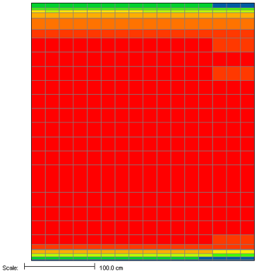
Fig. 5.4.2 MeshView plot of total plutonium content in the 3D depletion regions (XZ plane)

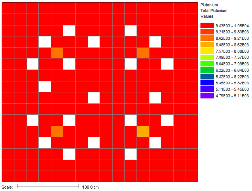
Fig. 5.4.3 MeshView plot of total plutonium content in the 3D depletion regions (XY plane).

5.4.6. Parallel Execution on Linux Clusters

For large 3D depletion problems it is advantageous to execute the ORIGEN calculations for different depletion regions in parallel. This can be done on Linux clusters using MPI. When parallel execution mode is enabled, ORIGAMI distributes the individual depletion cases across the pin rows, columns, and axial zones across several processors; the depletion calculation is thus split across several processors. ORIGAMI then collects the inventories from each calculation node and concatenates the output.

To execute ORIGAMI in parallel mode, a parallel-enabled MPI build of SCALE must be used and ORIGAMI should be invoked with the percent (%) prefix:

=%

<normal ORIGAMI input follows>

Additionally, for parallel jobs spanning multiple computational nodes (as opposed to those just using multiple processors on the same node, it is recommended to use the –T option to specify a common temporary directory (such as a network-mounted directory accessible to all nodes). This is due to the way ORIGAMI divides the problem space in parallel mode; each computational node stores its respective binary dump file of the individual pin/zone concentrations. Upon completion of execution, the master node must be able to locate these individual problem node-generated binary dump files; thus, by using a common temporary directory, ORIGAMI can correctly re-assembly the individual pinwise dumpfiles into a single consolidated “master” dump file.

The following is a typical execution command line to execute ORIGAMI in parallel.

scalerte –N [number of nodes] -M [machine file] –T [tmpdir] [input_file.inp]

For more information on executing SCALE in parallel, see the SCALE Readme file.

5.4.7. Sample Problems

This section shows sample problems for each of the three types of simulated assembly models: 0D fully lumped, 2D lumped axial depletion, and 3D pinwise depletion, and also demonstrates a restart case.

5.4.7.1. Sample problem 1: fully lumped assembly model

The first example, Example 5.4.10, corresponds to a fully-lumped assembly model in which the materials are depleted with a space-independent (i.e., assembly average) flux distribution. The assembly contains 0.38 MTU, and the fuel is 2.8 wt% enriched. The assembly also includes several non-fuel materials corresponding to cladding and other structural materials. Note that the non-fuel concentrations are specified in kg/MTU, and thus are not the actual total non-fuel masses in the 0.38 MTU assembly. The assembly is depleted for three cycles with specific powers of 40.0, 38.6, and 25.2 MW/MTU, respectively. The ORIGEN library data are interpolated for eight different burnup steps during the irradiation periods of the first two cycles, and for six burnup steps in the last cycle.

Table 5.4.10 gives the calculated actinide concentrations at the end of the third cycle.

Example 5.4.10 Input for ORIGAMI sample problem 1

 =origami
   title='fully lumped assembly model'
   libs=[ ce14x14 ]
   fuelcomp{
     stdcomp(fuel){
        base=uo2 iso[92234=0.02848 92235=3.2 92236=0.01472 92238=96.7568] }
        mix(1){ comps[fuel=100] }
    }
    options{ mtu=0.38 ft71=all }
    nonfuel=[ cr=3.366 mn=0.1525 fe=6.309 co=0.0302
              ni=2.366 zr=516.3 sn=8.412 gd=2.860 ]
    hist[
       cycle{ power=40 burn=284 nlib=4 down=54 }
       cycle{ power=38.6 burn=300 nlib=4 down=28 }
       cycle{ power=25.2 burn=250 nlib=3 down=30 }
    ]
    print{
       nuc {
           sublibs=[ac fp]
           units=[grams moles]
           total=no }
       }
 end

Table 5.4.10 Calculated Actinide inventories for sample problem 1
Nuclide *	Mass (g)
²³⁴U	6.820E+01
²³⁵U	3.621E+03
²³⁶U	1.487E+03
²³⁸U	3.598E+05
²³⁷Np	1.348E+02
²³⁸Pu	3.862E+01
²³⁹Pu	1.919E+03
²⁴⁰Pu	7.820E+02
²⁴¹Pu	3.960E+02
²⁴²Pu	1.394E+02
²⁴¹Am	1.474E+01
²⁴³Am	2.491E+01
²⁴²Cm	2.663E+00
²⁴⁴Cm	5.698E+00
TOTAL	6.820E+01

* Actinides with concentrations less than 0.0001 are not shown.

5.4.7.2. Sample problem 2: lumped axial depletion assembly model

The second example has the same lumped assembly and power history as sample problem 1, except in this case an axial power distribution is provided for eight zones, so that the fuel burnup will vary axially; the ORIGAMI input for this case is provided as Example 5.4.11. Also, the options to generate standard composition and decay output files are requested.

Table 5.4.11 gives the computed actinide concentrations in grams for the first four of the eight axial zones. Since the input axial power distribution is symmetrical about the assembly midplane, the last four zones have identical concentrations as the first four. The last column in the table shows actinide masses for the entire assembly.

Example 5.4.12 is a listing of the contents of the compBlock file, which contains standard composition input for the eight axial zones in the assembly at the end of cycle 3. A complete description of the SCALE standard composition input format is given in the XSPROC chapter The first entry on each line in Example 5.4.12 corresponds to the SCALE nuclide identifier. Only the default burnup credit analysis are included. The second entry is the mixture number associated with a particular axial zone. The mixture number for an axial zone is obtained using Eq. (5.4.14). The third entry is always zero in this file, and the fourth entry corresponds to the number density in atoms per barn-cm. The next entry on the line is the temperature, which has the default value of 293.0 since the input parameter temper was not specified. The final entry is an “end” statement. The information in this file can be used as the read comp input block for any SCALE module.

Example 5.4.13 shows a listing of the file AxialDecayHeat, which contains the heat source at the end of the third cycle. The entries in the file correspond to the decay power in watts for the eight axial zones, which are computed using Eq. (5.4.17).

Example 5.4.11 Input for ORIGAMI sample problem 2

 =origami
 title= 'lumped axial-deplete assembly model'
 libs=[ ce14x14 ]
 fuelcomp{
    uox(fuel2){ enrich=3.2 }
    mix(1){ comps[fuel2=100] }
 }
 options{
    mtu=0.38 stdcomp=yes decayheat=yes
  }
 pz=[ 1.0 2.0 3.0 4.0 4.0 3.0 2.0 1.0 ]
 nonfuel=[ cr=3.366 mn=0.1525 fe=6.309 co=0.0302
           ni=2.366 zr=516.3 sn=8.412 gd=2.860 ]
 hist[
    cycle{ power=40 burn=284 nlib=4 down=54 }
    cycle{ power=38.6 burn=300 nlib=4 down=28 }
    cycle{ power=25.2 burn=250 nlib=3 down=30 }
 ]
 end

Table 5.4.11 Calculated actinide inventories by axial zone for sample problem 2
Nuclide	Axial Zone 1 Mass (g)	Axial Zone 2 Mass (g)	Axial Zone 3 Mass (g)	Axial Zone 4 Mass (g)	TOTAL Mass (g)
²³⁴U	1.1384E+01	9.4326E+00	7.6666E+00	6.11E+00	6.92E+01
²³⁵U	9.7324E+02	5.9453E+02	3.3795E+02	1.78E+02	4.17E+03
²³⁶U	1.0392E+02	1.6544E+02	2.0053E+02	2.15E+02	1.37E+03
²³⁸U	4.5604E+04	4.5202E+04	4.4752E+04	4.43E+04	3.60E+05
²³⁷Np	4.7874E+00	1.2622E+01	2.0984E+01	2.83E+01	1.33E+02
²³⁸Pu	5.5445E-01	2.9024E+00	7.1722E+00	1.26E+01	4.65E+01
²³⁹Pu	1.7378E+02	2.2968E+02	2.4438E+02	2.46E+02	1.79E+03
²⁴⁰Pu	3.3124E+01	7.7894E+01	1.1457E+02	1.40E+02	7.30E+02
²⁴¹Pu	1.2974E+01	3.8401E+01	5.8714E+01	7.09E+01	3.62E+02
²⁴²Pu	1.4543E+00	1.0115E+01	2.6393E+01	4.75E+01	1.71E+02
²⁴¹Am	5.3938E-01	1.5121E+00	2.0433E+00	2.12E+00	1.24E+01
²⁴³Am	9.5029E-02	1.4341E+00	5.6093E+00	1.29E+01	4.00E+01
²⁴²Cm	< 0.0001	2.0213E-01	4.7744E-01	7.56E-01	2.93E+00
²⁴⁴Cm	< 0.0001	2.4685E-01	1.6315E+00	5.54E+00	1.49E+01
²⁴⁵Cm	< 0.0001	< 0.0001	5.8836E-02	2.40E-01	6.11E-01
TOTAL	4.6920E+04	4.6346E+04	4.5780E+04	4.5221E+04	3.6854E+05

Example 5.4.12 Sample Problem 2: Standard composition file (default burnup credit nuclides)

 o-16   1001 0 4.6395E-02 293.0 end
 u-234  1001 0 5.6529E-06 293.0 end
 u-235  1001 0 4.8120E-04 293.0 end
 u-236  1001 0 5.1165E-05 293.0 end
 u-238  1001 0 2.2263E-02 293.0 end
 np-237 1001 0 2.3470E-06 293.0 end
 pu-238 1001 0 2.7067E-07 293.0 end
 pu-239 1001 0 8.4481E-05 293.0 end
 pu-240 1001 0 1.6036E-05 293.0 end
 pu-241 1001 0 6.2547E-06 293.0 end
 pu-242 1001 0 6.9823E-07 293.0 end
 am-241 1001 0 2.6003E-07 293.0 end
 am-243 1001 0 4.5435E-08 293.0 end
 mo-95  1001 0 1.5700E-05 293.0 end
 tc-99  1001 0 1.7475E-05 293.0 end
 ru-101 1001 0 1.5272E-05 293.0 end
 rh-103 1001 0 9.4877E-06 293.0 end
 ag-109 1001 0 7.6473E-07 293.0 end
 cs-133 1001 0 1.8563E-05 293.0 end
 nd-143 1001 0 1.4504E-05 293.0 end
 nd-145 1001 0 1.0445E-05 293.0 end
 sm-147 1001 0 1.5451E-06 293.0 end
 sm-149 1001 0 8.0469E-08 293.0 end
 sm-150 1001 0 3.3359E-06 293.0 end
 sm-151 1001 0 3.5230E-07 293.0 end
 sm-152 1001 0 1.7469E-06 293.0 end
 eu-151 1001 0 1.5582E-09 293.0 end
 eu-153 1001 0 9.1077E-07 293.0 end
 gd-155 1001 0 1.3966E-09 293.0 end
 o-16   1002 0 4.6394E-02 293.0 end
 u-234  1002 0 4.6837E-06 293.0 end
 u-235  1002 0 2.9395E-04 293.0 end
 u-236  1002 0 8.1452E-05 293.0 end
 u-238  1002 0 2.2067E-02 293.0 end
 np-237 1002 0 6.1878E-06 293.0 end
 pu-238 1002 0 1.4169E-06 293.0 end
 pu-239 1002 0 1.1165E-04 293.0 end
 pu-240 1002 0 3.7710E-05 293.0 end
 pu-241 1002 0 1.8513E-05 293.0 end
 pu-242 1002 0 4.8561E-06 293.0 end
 am-241 1002 0 7.2896E-07 293.0 end
 am-243 1002 0 6.8566E-07 293.0 end
 mo-95  1002 0 2.9706E-05 293.0 end
 tc-99  1002 0 3.3424E-05 293.0 end
 ru-101 1002 0 3.0467E-05 293.0 end
 rh-103 1002 0 1.8486E-05 293.0 end
 ag-109 1002 0 2.2784E-06 293.0 end
 cs-133 1002 0 3.5311E-05 293.0 end
 nd-143 1002 0 2.4869E-05 293.0 end
 nd-145 1002 0 1.9393E-05 293.0 end
 sm-147 1002 0 2.4415E-06 293.0 end
 sm-149 1002 0 1.0154E-07 293.0 end
 sm-150 1002 0 7.3182E-06 293.0 end
 sm-151 1002 0 4.4543E-07 293.0 end
 sm-152 1002 0 3.4915E-06 293.0 end
 eu-151 1002 0 1.1064E-09 293.0 end
 eu-153 1002 0 2.5199E-06 293.0 end
 gd-155 1002 0 2.5157E-09 293.0 end
 o-16   1003 0 4.6392E-02 293.0 end
 u-234  1003 0 3.8068E-06 293.0 end
 u-235  1003 0 1.6709E-04 293.0 end
 u-236  1003 0 9.8728E-05 293.0 end
 u-238  1003 0 2.1847E-02 293.0 end
 np-237 1003 0 1.0287E-05 293.0 end
 pu-238 1003 0 3.5014E-06 293.0 end
 pu-239 1003 0 1.1880E-04 293.0 end
 pu-240 1003 0 5.5465E-05 293.0 end
 pu-241 1003 0 2.8306E-05 293.0 end
 pu-242 1003 0 1.2671E-05 293.0 end
 am-241 1003 0 9.8507E-07 293.0 end
 am-243 1003 0 2.6819E-06 293.0 end
 mo-95  1003 0 4.2205E-05 293.0 end
 tc-99  1003 0 4.7742E-05 293.0 end
 ru-101 1003 0 4.5361E-05 293.0 end
 rh-103 1003 0 2.6134E-05 293.0 end
 ag-109 1003 0 4.1770E-06 293.0 end
 cs-133 1003 0 5.0069E-05 293.0 end
 nd-143 1003 0 3.1519E-05 293.0 end
 nd-145 1003 0 2.6993E-05 293.0 end
 sm-147 1003 0 2.8511E-06 293.0 end
 sm-149 1003 0 1.2277E-07 293.0 end
 sm-150 1003 0 1.1691E-05 293.0 end
 sm-151 1003 0 5.2472E-07 293.0 end
 sm-152 1003 0 5.0112E-06 293.0 end
 eu-151 1003 0 9.0563E-10 293.0 end
 eu-153 1003 0 4.4446E-06 293.0 end
 gd-155 1003 0 4.0054E-09 293.0 end
 o-16   1004 0 4.6390E-02 293.0 end
 u-234  1004 0 3.0343E-06 293.0 end
 u-235  1004 0 8.7951E-05 293.0 end
 u-236  1004 0 1.0588E-04 293.0 end
 u-238  1004 0 2.1605E-02 293.0 end
 np-237 1004 0 1.3864E-05 293.0 end
 pu-238 1004 0 6.1605E-06 293.0 end
 pu-239 1004 0 1.1946E-04 293.0 end
 pu-240 1004 0 6.7542E-05 293.0 end
 pu-241 1004 0 3.4172E-05 293.0 end
 pu-242 1004 0 2.2786E-05 293.0 end
 am-241 1004 0 1.0210E-06 293.0 end
 am-243 1004 0 6.1463E-06 293.0 end
 mo-95  1004 0 5.3319E-05 293.0 end
 tc-99  1004 0 6.0395E-05 293.0 end
 ru-101 1004 0 5.9831E-05 293.0 end
 rh-103 1004 0 3.2151E-05 293.0 end
 ag-109 1004 0 6.2338E-06 293.0 end
 cs-133 1004 0 6.2779E-05 293.0 end
 nd-143 1004 0 3.4995E-05 293.0 end
 nd-145 1004 0 3.3350E-05 293.0 end
 sm-147 1004 0 2.9202E-06 293.0 end
 sm-149 1004 0 1.4469E-07 293.0 end
 sm-150 1004 0 1.6101E-05 293.0 end
 sm-151 1004 0 6.0099E-07 293.0 end
 sm-152 1004 0 6.3684E-06 293.0 end
 eu-151 1004 0 8.1899E-10 293.0 end
 eu-153 1004 0 6.4006E-06 293.0 end
 gd-155 1004 0 5.5315E-09 293.0 end
 o-16   1005 0 4.6390E-02 293.0 end
 u-234  1005 0 3.0343E-06 293.0 end
 u-235  1005 0 8.7951E-05 293.0 end
 u-236  1005 0 1.0588E-04 293.0 end
 u-238  1005 0 2.1605E-02 293.0 end
 np-237 1005 0 1.3864E-05 293.0 end
 pu-238 1005 0 6.1605E-06 293.0 end
 pu-239 1005 0 1.1946E-04 293.0 end
 pu-240 1005 0 6.7542E-05 293.0 end
 pu-241 1005 0 3.4172E-05 293.0 end
 pu-242 1005 0 2.2786E-05 293.0 end
 am-241 1005 0 1.0210E-06 293.0 end
 am-243 1005 0 6.1463E-06 293.0 end
 mo-95  1005 0 5.3319E-05 293.0 end
 tc-99  1005 0 6.0395E-05 293.0 end
 ru-101 1005 0 5.9831E-05 293.0 end
 rh-103 1005 0 3.2151E-05 293.0 end
 ag-109 1005 0 6.2338E-06 293.0 end
 cs-133 1005 0 6.2779E-05 293.0 end
 nd-143 1005 0 3.4995E-05 293.0 end
 nd-145 1005 0 3.3350E-05 293.0 end
 sm-147 1005 0 2.9202E-06 293.0 end
 sm-149 1005 0 1.4469E-07 293.0 end
 sm-150 1005 0 1.6101E-05 293.0 end
 sm-151 1005 0 6.0099E-07 293.0 end
 sm-152 1005 0 6.3684E-06 293.0 end
 eu-151 1005 0 8.1899E-10 293.0 end
 eu-153 1005 0 6.4006E-06 293.0 end
 gd-155 1005 0 5.5315E-09 293.0 end
 o-16   1006 0 4.6392E-02 293.0 end
 u-234  1006 0 3.8068E-06 293.0 end
 u-235  1006 0 1.6709E-04 293.0 end
 u-236  1006 0 9.8728E-05 293.0 end
 u-238  1006 0 2.1847E-02 293.0 end
 np-237 1006 0 1.0287E-05 293.0 end
 pu-238 1006 0 3.5014E-06 293.0 end
 pu-239 1006 0 1.1880E-04 293.0 end
 pu-240 1006 0 5.5465E-05 293.0 end
 pu-241 1006 0 2.8306E-05 293.0 end
 pu-242 1006 0 1.2671E-05 293.0 end
 am-241 1006 0 9.8507E-07 293.0 end
 am-243 1006 0 2.6819E-06 293.0 end
 mo-95  1006 0 4.2205E-05 293.0 end
 tc-99  1006 0 4.7742E-05 293.0 end
 ru-101 1006 0 4.5361E-05 293.0 end
 rh-103 1006 0 2.6134E-05 293.0 end
 ag-109 1006 0 4.1770E-06 293.0 end
 cs-133 1006 0 5.0069E-05 293.0 end
 nd-143 1006 0 3.1519E-05 293.0 end
 nd-145 1006 0 2.6993E-05 293.0 end
 sm-147 1006 0 2.8511E-06 293.0 end
 sm-149 1006 0 1.2277E-07 293.0 end
 sm-150 1006 0 1.1691E-05 293.0 end
 sm-151 1006 0 5.2472E-07 293.0 end
 sm-152 1006 0 5.0112E-06 293.0 end
 eu-151 1006 0 9.0563E-10 293.0 end
 eu-153 1006 0 4.4446E-06 293.0 end
 gd-155 1006 0 4.0054E-09 293.0 end
 o-16   1007 0 4.6394E-02 293.0 end
 u-234  1007 0 4.6837E-06 293.0 end
 u-235  1007 0 2.9395E-04 293.0 end
 u-236  1007 0 8.1452E-05 293.0 end
 u-238  1007 0 2.2067E-02 293.0 end
 np-237 1007 0 6.1878E-06 293.0 end
 pu-238 1007 0 1.4169E-06 293.0 end
 pu-239 1007 0 1.1165E-04 293.0 end
 pu-240 1007 0 3.7710E-05 293.0 end
 pu-241 1007 0 1.8513E-05 293.0 end
 pu-242 1007 0 4.8561E-06 293.0 end
 am-241 1007 0 7.2896E-07 293.0 end
 am-243 1007 0 6.8566E-07 293.0 end
 mo-95  1007 0 2.9706E-05 293.0 end
 tc-99  1007 0 3.3424E-05 293.0 end
 ru-101 1007 0 3.0467E-05 293.0 end
 rh-103 1007 0 1.8486E-05 293.0 end
 ag-109 1007 0 2.2784E-06 293.0 end
 cs-133 1007 0 3.5311E-05 293.0 end
 nd-143 1007 0 2.4869E-05 293.0 end
 nd-145 1007 0 1.9393E-05 293.0 end
 sm-147 1007 0 2.4415E-06 293.0 end
 sm-149 1007 0 1.0154E-07 293.0 end
 sm-150 1007 0 7.3182E-06 293.0 end
 sm-151 1007 0 4.4543E-07 293.0 end
 sm-152 1007 0 3.4915E-06 293.0 end
 eu-151 1007 0 1.1064E-09 293.0 end
 eu-153 1007 0 2.5199E-06 293.0 end
 gd-155 1007 0 2.5157E-09 293.0 end
 o-16   1008 0 4.6395E-02 293.0 end
 u-234  1008 0 5.6529E-06 293.0 end
 u-235  1008 0 4.8120E-04 293.0 end
 u-236  1008 0 5.1165E-05 293.0 end
 u-238  1008 0 2.2263E-02 293.0 end
 np-237 1008 0 2.3470E-06 293.0 end
 pu-238 1008 0 2.7067E-07 293.0 end
 pu-239 1008 0 8.4481E-05 293.0 end
 pu-240 1008 0 1.6036E-05 293.0 end
 pu-241 1008 0 6.2547E-06 293.0 end
 pu-242 1008 0 6.9823E-07 293.0 end
 am-241 1008 0 2.6003E-07 293.0 end
 am-243 1008 0 4.5435E-08 293.0 end
 mo-95  1008 0 1.5700E-05 293.0 end
 tc-99  1008 0 1.7475E-05 293.0 end
 ru-101 1008 0 1.5272E-05 293.0 end
 rh-103 1008 0 9.4877E-06 293.0 end
 ag-109 1008 0 7.6473E-07 293.0 end
 cs-133 1008 0 1.8563E-05 293.0 end
 nd-143 1008 0 1.4504E-05 293.0 end
 nd-145 1008 0 1.0445E-05 293.0 end
 sm-147 1008 0 1.5451E-06 293.0 end
 sm-149 1008 0 8.0469E-08 293.0 end
 sm-150 1008 0 3.3359E-06 293.0 end
 sm-151 1008 0 3.5230E-07 293.0 end
 sm-152 1008 0 1.7469E-06 293.0 end
 eu-151 1008 0 1.5582E-09 293.0 end
 eu-153 1008 0 9.1077E-07 293.0 end
 gd-155 1008 0 1.3966E-09 293.0 end

Example 5.4.13 Sample problem 2: Decay heat file with axial decay heat by zone (Watts)

11397E+02
43786E+03
18631E+03
95428E+03
95428E+03
18631E+03
43786E+03
11397E+02

5.4.7.3. Sample problem 3: restart decay calculation for lumped axial depletion assembly model

The third example shows a restart decay-only calculation, using the ORIGEN ft71 binary file obtained from sample problem 2. This case calculates the composition of the burned fuel produced in sample problem 2 after 100,000 additional days of decay. The input this problem is given in Example 5.4.15. Because the input parameter restart=yes is specified, the initial composition of the assembly is obtained from a file named assembly_restart.f71. The shell input that precedes the ORIGAMI input in Example 5.4.15 copies the output ft71 file produced in sample problem 2, which was named assembly_dump.f71, into a file named assembly_restart.f71 in the temporary directory for SCALE calculations. The restart file contains the complete inventory of nuclide compositions for eight axial zones. Because this restart case is decay only (i.e., power value is not given in the power-history block), it is necessary to provide the input parameter nz=8 because this value is used to determine how many axial zones were used in the previous burnup calculations.

Table 5.4.12 shows the actinide composition of the first four axial of the (symmetrical) eight zones after 100,000 days of decay. The initial masses of these nuclides before decay are the values given in numref:ex-origami-prob2-stdcmp. The last column in Table 5.4.12 shows actinide masses for the entire assembly after the decay period.

Example 5.4.14 Sample problem 3: restart decay for a lumped axial depletion model

 =origami
    title= 'lumped axial-deplete assembly model'
    libs=[ ce14x14 ]
    fuelcomp{
       %3.2 w/o
       uox(fuel){ enrich=3.2 }
       mix(1){ comps[fuel=100] }
    }
    options[ mtu=0.38 relnorm=no ]
    pz=[ 1.0 2.0 3.0 4.0 4.0 3.0 2.0 1.0 ]
    nonfuel=[ cr=3.366 mn=0.1525 fe=6.309 co=0.0302
              ni=2.366 zr=516.3 sn=8.412 gd=2.860 ]
    hist[
       cycle{ power=40 burn=284 nlib=8 down=54 }
       cycle{ power=38.6 burn=300 nlib=8 down=28 }
       cycle{ power=25.2 burn=250 nlib=6 down=30 }
    ]
    end
    =shell
       mv \*.assm.f71 assembly_restart.f71
    end
    =origami
       title= 'restart decay'
       asmid= 22
       libs=[ ce14x14 ]
       prefix=origam3
    options{
       stdcomp=yes decayheat=yes relnorm=no restart=yes nz=8
    }
    pz=[ 1.0 2.0 3.0 4.0 4.0 3.0 2.0 1.0 ]
    hist[
       cycle{ down=100000 }
    ]
    end
    =shell
       rm assembly_restart.f71
       rm ${OUTDIR}/\*origam3\*
    end

Table 5.4.12 Calculated actinide inventories by axial zone for sample problem 3
Nuclide	Axial Zone 1 Mass (g)	Axial Zone 2 Mass (g)	Axial Zone 3 Mass (g)	Axial Zone 4 Mass (g)	TOTAL Mass (g)
²³⁴U	1.1889E+01	1.2133E+01	1.4319E+01	1.7738E+01	1.1216E+02
²³⁵U	9.7454E+02	5.9616E+02	3.3963E+02	1.7955E+02	4.1798E+03
²³⁶U	1.0486E+02	1.6764E+02	2.0378E+02	2.1907E+02	1.3907E+03
²³⁸U	4.5604E+04	4.5202E+04	4.4752E+04	4.4256E+04	3.5963E+05
²³⁷Np	9.2242E+00	2.5723E+01	4.0929E+01	5.2246E+01	2.5625E+02
²³⁸Pu	6.8535E-02	3.6104E-01	8.8478E-01	1.5422E+00	5.7132E+00
²³⁹Pu	1.7243E+02	2.2794E+02	2.4262E+02	2.4413E+02	1.7742E+03
²⁴⁰Pu	3.2192E+01	7.5957E+01	1.1297E+02	1.4095E+02	7.2412E+02
²⁴¹Pu	< 0.0001	< 0.0001	< 0.0001	< 0.0001	< 0.0001
²⁴²Pu	1.4538E+00	1.0107E+01	2.6379E+01	4.7456E+01	1.7079E+02
²⁴¹Am	8.9945E+00	2.6564E+01	4.0451E+01	4.8623E+01	2.4927E+02
²⁴³Am	9.2577E-02	1.3965E+00	5.4616E+00	1.2516E+01	3.8934E+01
²⁴²Cm	< 0.0001	< 0.0001	< 0.0001	< 0.0001	< 0.0001
²⁴⁴Cm	< 0.0001	< 0.0001	< 0.0001	< 0.0001	< 0.0001
²⁴⁵Cm	< 0.0001	< 0.0001	5.7288E-02	2.3382E-01	5.9479E-01
TOTAL	4.6920E+04	4.6346E+04	4.5780E+04	4.5220E+04	3.6853E+05

5.4.7.4. Sample problem 4: Simplified 3D multi-pin model

The fourth example is a simulation of a simplified 3D depletion model. The ORIGAMI 3D model normally includes all fuel pins within the assembly, such as a 14×14 array. However to keep this example case simple and the execution time low, only a 2×2 array of four individual pins is considered for illustrative purposes. An axial fractional power distribution is also specified for two axial zones. Therefore the total number of depletion regions will be eight – two axial for each of the four pins. Two different ORIGEN libraries are used to obtain cross sections for the four pins. This is done whenever fuel pins in different locations in the assembly have significantly different neutron spectra, such as if some pins are adjacent to a control rod. In this sample problem, ORIGEN libraries for two different types of assembly designs CE (Combustion Engineering) 14×14 and 16×16 assembly designs, respectively are used to demonstrate the use of pin-dependent libraries, although in reality the ORIGEN libraries normally would be pre-generated for different pin locations within a single type of assembly configuration. The values specified in libmap indicate which library is to be used for each pin location. Example 5.4.15 shows the input for this sample problem.

Example 5.4.15 Input for ORIGAMI Sample Problem 4: a simplified multi-pin, multi-axial model

 =origami
  title= 'multi-pin; multi-library pin-deplete model'
  prefix= origam4
  libs=[ ce14x14 ce16x16 ]

  fuelcomp{
     %3.2 w/o
     stdcomp(fuel){ base=uo2 iso[92234=0.028569 92235=3.21 92236=0.014766
                                92238=96.746665] }
     mix(1){ comps[fuel=100] }
  }

  options{ mtu=0.4 decayheat=yes }
  libmap=[ 1 1
           2 2 ]
  pxy=[ 0.284 0.283
        0.218 0.215 ]
  pz=[ 0.55 0.45 ]
  hist[
    cycle{ power=39.78 burn=284.0 nlib=2 down=54.0 }
  ]
 end

Table 5.4.13 shows selected actinide compositions for the first row of two pins, that is, locations (1,1) and (1,2), for each of the two axial zones. The blended compositions over all fuel pins, for the two axial zones, are given in Table 5.4.14. The output decay heat file for the assembly is shown in Table 5.4.15, as a function of axial zone, summed over all pins. Note that this file has the prefix “sample4_” appended to the standard file name, since prefix=sample4 is specified in the input.

Table 5.4.13 Actinide inventories by axial zone for pins (1,1) and (1,2) in sample problem 4
Nuclide	pin (1,1) Axial Zone 1 Mass (g)	pin (1,1) Axial Zone 2 Mass (g)	pin (1,2) Axial Zone 1 Mass (g)	pin (1,2) Axial Zone 2 Mass (g)
²³⁴U	1.2115E+01	1.2493E+01	1.2143E+01	1.2516E+01
²³⁵U	1.0701E+03	1.1528E+03	1.0762E+03	1.1581E+03
²³⁶U	1.0383E+02	8.9286E+01	1.0277E+02	8.8348E+01
²³⁷U	1.0664E-03	< 0.0001	1.0428E-03	< 0.0001
²³⁸U	4.8003E+04	4.8074E+04	4.8009E+04	4.8078E+04
²³⁷Np	4.8000E+00	3.6009E+00	4.7055E+00	3.5303E+00
²³⁹Np	5.8742E-07	4.4485E-07	5.7555E-07	4.3692E-07
²³⁸Pu	4.7198E-01	2.9453E-01	4.5684E-01	2.8512E-01
²³⁹Pu	1.8855E+02	1.6706E+02	1.8705E+02	1.6560E+02
²⁴⁰Pu	3.3235E+01	2.5225E+01	3.2625E+01	2.4736E+01
²⁴¹Pu	1.3906E+01	9.2953E+00	1.3537E+01	9.0304E+00
²⁴²Pu	1.3733E+00	7.3260E-01	1.3161E+00	7.0081E-01
²⁴¹Am	2.3603E-01	1.5773E-01	2.2978E-01	1.5322E-01
²⁴³Am	8.4143E-02	< 0.0001	7.9365E-02	< 0.0001
TOTAL	4.9432E+04	4.9535E+04	4.9440E+04	4.9541E+04

4: Values < 0.0001 are not shown

Table 5.4.14 Blended actinide inventories by axial zone (all pins) for sample problem 4
Nuclide	Axial Zone 1 Mass (g)	Axial Zone 2 Mass (g)	TOTAL Mass (g)
²³⁴U	4.7388E+01	4.9082E+01	9.6469E+01
²³⁵U	4.0115E+03	4.3778E+03	8.3894E+03
²³⁶U	4.5851E+02	3.9537E+02	8.5387E+02
²³⁸U	1.9184E+05	1.9216E+05	3.8399E+05
²³⁷Np	2.2821E+01	1.7132E+01	3.9953E+01
²³⁸Pu	2.5739E+00	1.6049E+00	4.1789E+00
²³⁹Pu	7.8246E+02	6.9963E+02	1.4821E+03
²⁴⁰Pu	1.5436E+02	1.1801E+02	2.7238E+02
²⁴¹Pu	6.7918E+01	4.6455E+01	1.1437E+02
²⁴²Pu	8.1693E+00	4.4411E+00	1.2610E+01
²⁴¹Am	1.1476E+00	7.8696E-01	1.9346E+00
²⁴³Am	6.0150E-01	2.5995E-01	8.6145E-01
TOTAL	1.9740E+05	1.9787E+05	3.9526E+05

Table 5.4.15 Sample problem 4: Decay heat by axial zone (Watts)
6.96472E+03 5.72539E+03

5.4.7.5. Sample problem 5: PWR 3D assembly model

This sample problem shows the input for a simulated full 3D pressurized water reactor (PWR) assembly-depletion model, which corresponds to a 16×16 lattice with 26 axial zones. Example 5.4.16 shows the ORIGAMI input for this case. The arrays pxy and pz define the 3D XY-Z fractional power distribution. Four different pre-processed ORIGEN libraries are used to describe the pin-averaged ORIGEN cross-sections for the assembly. The array libmap assigns these libraries to the appropriate pin locations. It can be seen that the libmap array contains values of zero at 21 locations. These correspond to non-depleting (i.e., zero power) locations. The input includes the information (parameter pitch, and array z= ) necessary to generate 3D mesh summary maps for subsequent visualization. In this case, the axial mesh is not uniform. Since a total of 6110 ORIGEN cases are executed for the depletable pins, this ORIGAMI calculation was performed in parallel using MPI. Figure 5.4.3 shows a plot of the axial burnup distribution, summed over all pins.

Example 5.4.16 Input for ORIGAMI Sample Problem 4

  =%origami
  title= 'PWR 3D deplete model'
  prefix= pwr
  options{ pitch= 19.816 }
  fuelcomp{
  uox(fuel){ enrich=3.5 }
     mix(1){ comps[fuel=100] }
  }
  libs=[ lib1 lib2 lib3 lib4]
  libmap=[
2 2 2 2 2 2 2 2 2 2 2 2 2 2 3
1 1 1 1 4 1 1 1 1 4 1 1 1 1 2
1 1 4 4 0 4 4 1 4 0 4 4 1 1 2
1 4 0 4 4 4 0 4 1 4 4 0 4 1 2
1 4 4 1 4 1 4 1 1 4 1 4 4 1 2
4 0 4 4 0 4 1 1 4 0 4 4 0 4 2
1 4 4 1 4 1 1 1 1 4 1 1 4 1 2
1 4 0 4 1 1 4 1 1 1 1 4 1 1 2
1 1 4 1 1 4 0 4 1 1 4 0 4 1 2
1 4 1 1 4 1 4 1 1 4 1 4 4 1 2
4 0 4 4 0 4 1 1 4 0 4 4 0 4 2
1 4 4 1 4 1 4 1 1 4 1 4 4 1 2
1 4 0 4 4 4 0 4 1 4 4 0 4 1 2
1 1 4 4 0 4 4 1 4 0 4 4 1 1 2
1 1 1 1 4 1 1 1 1 4 1 1 1 1 2
2 2 2 2 2 2 2 2 2 2 2 2 2 2 3 ]
  pxy=[
99 0.98 0.98 0.99 0.99 0.99 0.99 0.99
99 0.99 0.99 0.99 0.98 0.98 0.97 0.98
99 0.99 0.99 1.00 1.01 1.02 1.00 1.00
00 1.01 1.02 1.00 0.99 0.98 0.98 0.98
00 1.00 1.01 1.03 1.03 0.00 1.03 1.01
03 1.04 0.00 1.03 1.02 1.00 0.99 0.98
01 1.01 1.03 0.00 1.04 1.04 1.02 0.00
03 1.04 1.04 1.04 0.00 1.02 1.00 0.99
01 1.02 1.02 1.05 0.73 1.04 1.02 1.02
03 1.03 1.04 0.72 1.04 1.04 1.01 1.00
02 1.04 0.00 1.05 1.04 0.00 1.03 1.01
01 1.03 0.00 1.03 1.04 0.00 1.02 1.00
02 1.03 1.02 1.05 1.04 1.04 1.02 1.01
01 1.02 1.03 1.02 1.02 1.03 1.01 1.00
01 1.02 1.04 0.00 1.04 1.02 1.02 1.03
01 1.01 1.01 1.02 1.03 1.02 1.00 1.00
00 1.01 1.02 1.03 1.02 1.02 1.03 0.00
02 1.01 1.01 1.03 0.00 1.02 0.99 0.98
00 1.01 1.03 1.02 1.02 1.03 1.03 1.03
01 1.01 1.03 1.02 1.03 1.03 1.00 0.99
01 1.02 0.00 1.04 1.03 0.00 1.03 1.01
01 1.02 0.00 1.03 1.03 0.00 1.01 0.98
00 1.01 1.04 1.04 0.72 1.04 1.03 1.03
01 1.01 1.02 0.71 1.03 1.02 0.99 0.98
00 1.00 1.02 0.00 1.04 1.04 1.04 0.00
02 1.01 1.03 1.03 0.00 1.01 0.98 0.97
99 0.99 1.01 1.03 1.04 0.00 1.04 1.03
01 1.02 0.00 1.02 1.01 0.99 0.97 0.97
99 0.99 0.99 1.00 1.01 1.03 1.01 1.00
00 1.00 1.01 1.00 0.99 0.97 0.97 0.97
00 0.99 1.00 1.00 1.01 1.01 1.01 1.00
99 0.99 0.99 0.99 0.98 0.97 0.97 0.97 ]

  pz=[0.486645842
510544887
641121243
798557507
931372279
063949280
173174524
178015382
241701554
247451593
203231683
228462686
237668911
221002529
191997899
231513011
222065701
172711869
200902470
164812132
083204453
931028309
810656652
700324838
611466339
516416427 ]

  meshz=[ 0.0 2.0 6.0 10.0 16.5 23.0 37.0 57.0 77.0 97.0 16.0
          136.0 156.0 176.0 196.0 216.0 236.0 256.0 276.0 296.0
          316.0 328.5 344.0 352.0 355.5 359.0 366.0 ]
  hist[
     cycle{ power=49.395 burn=385 nlib=3 down=52 }
     cycle{ power=43.772 burn=360 nlib=2 down=7673 }
  ]
  end

References

ORIGAMIOWHR94: O. W. Hermann, C. V. Parks and J. P. Renier. Technical Support for a Proposed Decay Heat Guide Using SAS2H/ORIGEN Data. Technical Report NUREG/CR-5625 (ORNL-6698), Martin Marietta Energy Systems, Inc., Oak Ridge National Laboratory, 9 1994.
ORIGAMIRGI10: G. Radulescu, I. C. Gauld, and G. Ilas. SCALE 5.1 Predictions of PWR Spent Nuclear Fuel Isotopic Compositions. Technical Report ORNL/TM-2010/44, Oak Ridge National Laboratory, Oak Ridge, TN (USA), 3 2010.
ORIGAMIRGlW12(1,2): G. Radulescu, I. C. Gauld, G. llas, and J. C. Wagner. An Approach for Validating Actinide and Fission Product Burnup Credit Criticality Safety Analyses-Isotopic Composition Predictions. Technical Report NUREG/CR-7108, ORNL/TM-2011/509, Oak Ridge National Laboratory, Oak Ridge, TN (USA), 4 2012.
ORIGAMISGRT12: S. Skutnik, I.C. Gauld, C.E. Romano, and H.R. Trellue. Creating NDA 'Working Standards' through High-Fidelity Spent Fuel Modeling. In Proceedings of the Institute of Nuclear Materials Management, 53rd Annual Meeting. Orlando, FL, 7 2012.
ORIGAMISHDLG13(1,2): S. Skutnik, F. Havlůj, D. Lago, and I. Gauld. Development of an Object-Oriented ORIGEN for Advanced Nuclear Fuel Modeling Applications. In International Conference on Mathematics and Computational Methods Applied to Nuclear Science & Engineering (M&C 2013). Sun Valley, ID, 5 2013.

Array Name	Description	Default
libs *	List of ORIGEN library file names for fuel in assembly. [characters]	None
libmap	XY map of library identifiers associated with each pin in assembly. Library identifiers correspond to the order of the ORIGEN libraries entered in the libs block. [integers]	1
compmap	XY map of mixture identifiers that correspond to the mixture ID in the `fuelcomp` block. [integers]	1
pxy	XY map of pin power shaping factors / fractional powers. Must be a square array (e.g., 15×15). Defaults to lumped assembly model (no individual pins). [real numbers]	1.0
pz	Axial (Z) power shaping factors / fractional power distribution for the assembly. [real numbers]	1.0
meshz	Axial mesh boundaries (cm) for the axial relative power zones. Only required to define axial mesh for viewing results; but if entered, it must be consistent with axial power shape. The number of entries should be one greater than number of entries in `pz` array. [real numbers]	None
modz	Axial variation in water density (g/cc) corresponding to the axial power zones. [real numbers]	0.723
nonfuel	Non-fuel materials contained in assembly. Values are entered in pairs of (element-symbol=mass(kg) per mtu of HM ). If parameter fracnf is input, mass of non-fuel materials is normalized to this fraction of fuel mtu. NOTE: Oxygen mass in UO₂ should not be entered here (i.e., this is pre-supplied by ORIGAMI). [character / real number pairs]	None
ggrp	Energy boundaries (eV) for defining decay gamma source spectrum. [real numbers]	None
ngrp	Energy boundaries (eV) for defining \(\left(\alpha,n\right)\) and fission neutron source spectrum. [real numbers]	None
nuccomp	List of nuclide IZZZAAAs to be included in output compBlock file.	Table 5.4.9 Nuclides
* indicates required