7.1. XSPROC: The Material and Cross Section Processing Module for SCALE
M. L. Williams, L. M. Petrie, R. A. Lefebvre, K. T. Clarno, J. P. Lefebvre, U. Merturyek, D. Wiarda, and B. T. Rearden
ABSTRACT
The material and cross section processing module of SCALE (XSProc) was improved for the 6.2 release to prepare data for continuous-energy and multigroup calculations. XSProc expands material input from Standard Composition Library definitions into atom number densities and, for multigroup calculations, performs cross section resonance self-shielding, energy group collapse, and spatial homogenization. XSProc implements capabilities for problem-dependent temperature interpolation, calculation of Dancoff factors, resonance self-shielding using Bondarenko factors with full-range intermediate resonance treatment, as well as use of continuous energy resonance self-shielding in the resolved resonance region. The SCALE 6.3 XSProc maintains the same architecture with SCALE 6.2 which integrated and enhanced the capabilities previously implemented independently in BONAMI, CENTRM, PMC, WORKER, ICE, and XSDRNPM, along with some additional capabilities that were provided by MIPLIB and SCALELIB. The SCALE 6.3 XSProc development focuses on improving accuracy, applicability and stability for any advanced reactor analysis including Light Water Reactors (LWR), Pebble and Prismatic High Temperature Gas-cooled Reactors (HTGR), Molten Salt Reactors (MSR), Sodium- and Lead-cooled Fast Reactors (SFR and LFR) without any limitation.
ACKNOWLEDGMENTS
Development and maintenance of XSProc and related codes and methods have been sponsored by the US Nuclear Regulatory Commission (NRC) and the US Department of Energy (DOE).
VERSION INFORMATION
XSProc has evolved from the concept of a Material Information Processor library (MIPLIB) that used alphanumeric material specifications, which was initially proposed and developed by R. M. Westfall. J. R. Knight and J. A. Bucholz expanded and refined MIPLIB in early SCALE releases.
SCALE 6.1 (2011) and 6.2 (2016): M. L. Williams and L. M. Petrie led development and improvement for XSProc and contributors include, R. A. Lefebvre, K. T. Clarno, J. P. Lefebvre, U. Merturyek, D. Wiarda, B. T. Rearden, S. Goluoglu, D. F. Hollenbach, N. F. Landers, J. A. Bucholz, C. F. Weber, and C. M. Hopper. With the SCALE modernization initiative beginning in SCALE 6.2, MIPLIB is no longer part of the XSProc analysis, but the original concepts and input formatting were preserved in the new implementation.
SCALE 6.3 (2021): K. S. Kim led responsibility and contributors include A. M. Holcomb, D. Wiarda, R. Bostelmann, M. A. Jessee, and W. A. Wieselquist. The SCALE 6.3 XSProc has been focused on improving accuracy, applicability and stability for advanced reactor analysis including high temperature gas cooled reactors and fast spectrum reactors.
7.1.1. Introduction
Self-shielding of multigroup cross sections is required in SCALE sequences for criticality safety, reactor physics, radiation shielding, and sensitivity analysis. In all previous versions of SCALE, resonance self-shielding calculations were done by executing a series of stand-alone executable codes, each dedicated to a specific aspect of the self-shielding operations. Each sequence had its own unique internal coding to launch the executable codes. Multigroup (MG) and continuous-energy (CE) cross sections and other data were passed between the individual executable codes by external I/O, which could require a substantial amount of clock time. In the modern version of SCALE, all self-shielding operations are consolidated into a single driver module named XSProc, and the stand-alone executable codes have been transformed into callable “computational modules” [XSProc-RLL+15]. The functions of XSProc are to (a) read input data, (b) generate in-memory data structures (objects) containing problem-definition information (compositions, cell geometries, computation options), as well as self-shielding information (MG and CE cross sections and fluxes), and (c) execute appropriate computational modules for the requested self-shielding option. Calculated results produced by one module may be stored in the internal data objects and passed to other modules through application program interfaces (APIs). At the completion of XSProc the self-shielded MG cross sections on the data objects can be passed along to transport solvers for continued execution of the control sequence or can be written to an external AMPX library file.
In the future, XSProc will be extended to parallel computations in which self-shielding calculations are done simultaneously for multiple types of unit cells. At the present time, however, XSProc is limited to serial computations; but even in serial mode it typically requires less time than older versions of SCALE to process shielded cross sections, and significant speedups have been observed for heavily I/O bound problems. Integrating the self-shielding capabilities into a single module has a number of additional benefits as well, including maintainability, extensibility, and the ability to easily replace an entire computational module with a future implementation containing new features. Additionally, the size of the problem-dependent MG library generated by XSProc may be greatly reduced compared to previous versions of SCALE because macroscopic cross sections are stored rather than a general-purpose library of microscopic data.
7.1.2. Techniques
XSProc integrates and enhances the capabilities previously implemented independently in BONAMI, CENTRM, PMC, WORKER, ICE, and XSDRNPM, as well as other capabilities formerly provided by MIPLIB and SCALELIB. It provides capabilities for problem-dependent temperature interpolation of both CE and MG nuclear data, calculation of Dancoff factors, and resonance self-shielding of MG cross sections using several available options. XSProc produces shielded microscopic data for each nuclide or macroscopic data for each material. Additionally, a flux-weighting spectrum can be applied to collapse cross sections to a coarser group structure and/or to integrate over volumes for homogenized cross sections. The flux-weighting spectrum can be input by the user or calculated using one-dimensional (1-D) coupled neutron/gamma transport model. These operations are performed by the sequences CSAS-MG, CSAS1, CSASI, and T-XSEC described in Sect. 7.1.3.2.
7.1.2.1. Overview of XSProc procedures
XSProc reads the COMPOSITION and CELL DATA blocks of the SCALE input, which are described in the following sections. After reading the user input data, XSProc loads the specified MG library to be self-shielded and, depending on the selected self-shielding method, additional CE data files for nuclides appearing in the problem specification. Finally XSProc performs MG self-shielding calculations for all compositions by calling APIs to computational modules such as BONAMI (BONdarenko AMPX Interpolator), CRAWDAD (Code to Read And Write DAta for Discretized solution), CENTRM (Continuous ENergy TRansport Module), PMC (Produce Multigroup Cross sections), CHOPS (Compute HOmogenized Pointwise Stuff), CAJUN (CE AJAX UNiter), WAX (Working AJAX), XSDRNPM (X-Section Development for Reactor Nucleonics with Petrie Modifications), and/or MIXMACRO to provide a problem-dependent cross section library. Many computational modules have been modernized compared to earlier executable codes distributed in previous versions of SCALE.
Like earlier versions of SCALE, XSProc provides several options for self-shielding an input MG library [XSProc-Wil11]. The first, based on the Bondarenko method [XSProc-IB64], uses the computational module BONAMI. BONAMI is always used to compute self-shielded cross sections for all energy groups. If parm=bonami is specified, the shielded cross sections provided by BONAMI are the final values output from XSProc. However the Bondarenko method has several limitations, especially in the resolved resonance range. Therefore XSProc provides another self-shielding method, with several computation options, which often produces more accurate MG data in the resolved resonance and thermal energy ranges. If parm=centrm or parm=2region is specified on the sequence line, XSProc calls APIs for the modules CRAWDAD, CENTRM, and PMC to compute CE flux spectra for processing problem-specific, self-shielded cross sections “on the fly [XSProc-WA95]. CENTRM performs MG transport calculations in the fast and lower energy ranges, coupled to pointwise (PW) transport calculations that use CE cross sections in the resonance range. PMC uses the PW flux spectra from CENTRM to compute MG values, which replace the previous values obtained from BONAMI over the specified range of the CE calculation. The original BONAMI shielded cross sections are retained for all other groups.
The CENTRM/PMC approach is the default for criticality and lattice physics calculations, while the BONAMI-only method is default for radiation shielding calculations. The end results of an XSProc calculation are self-shielded macroscopic and/or microscopic MG cross sections stored in memory for subsequent transport calculations; or alternatively a shielded MG AMPX library can be written to an external file and saved for future use.
7.1.2.2. Standard composition material processing
A primary function of the XSProc module is to expand user input in the COMPOSITION block into nuclear number densities (nuclei/b-cm) for every nuclide in each defined mixture. Mixtures can be specified through the direct use of materials presented in the Standard Composition Library, which includes individual nuclides, elements with natural abundances, numerous compounds, alloys and mixtures found in engineering practice, as well several variations of fissile solutions. Additionally, users may define their own materials as atom percent or weight percent combinations. Nuclear masses and theoretical densities are provided in the Standard Composition Library, and methods are available to determine equilibrium states for fissile solutions. Input options for composition data are described in Sect. 7.1.3.3 with several examples provided in Appendix A.
7.1.2.3. Unit cells for MG resonance self-shielding
XSProc utilizes a unit cell description to provide information for resonance self-shielding calculations of the input mixtures. As many unit cells as needed to describe the problem may be specified; however, each mixture (other than 0 for a void mixture) can appear only in one unit cell in the CELLDATA block. If a nuclide appears in more than one mixture, multiple sets of self-shielded cross sections are calculated for the nuclide-one for each mixture in each unit cell. Four types of cells are available for self-shielding calculations: INFHOMMEDIUM, LATTICECELL, MULTIREGION, and DOUBLEHET. The default calculation type is CENTRM/PMC for CSAS, TRITON, and TSUNAMI sequences and BONAMI for MAVRIC. All materials not specified in a unit cell are treated as infinite homogeneous media and shielded with BONAMI only, unless the mixture contains a fissionable nuclide, in which case an infinite medium CENTRM/PMC model is used. Note that previous versions of SCALE used infinite medium CENTRM/PMC calculations for all unassigned mixtures. The default type of self-shielding calculation can be overridden, as described in Sect. 7.1.3.2. The following is a brief description of the types of unit cells that can be input in CELLDATA and the computation procedures used.
7.1.2.3.1. INFHOMMEDIUM (infinite homogeneous medium) Treatment
The INFHOMMEDIUM treatment is best suited for large masses of materials where the size of each material is large compared with the average mean-free path of the material or where the fraction of the material that is a mean-free path from the surface of the material is very small. When INFHOMMEDIUM cell is specified, the material in the unit cell is treated as an infinite homogeneous lump. Systems composed of small fuel lumps or resonance nuclides sandwiched between moderating regions should not be treated as infinite homogeneous media. In these cases a MULTIREGION or LATTICECELL geometry should be used.
7.1.2.3.2. LATTICECELL Treatment
The LATTICECELL model is appropriate for arrays of resonance absorber mixtures-with or without clad-arranged in a square or a triangular pitch configuration within a moderator. Annular fuel (e.g., with an internal moderator in the center) can also be addressed. Input data for the LATTICECELL treatment are described in Sect. 7.1.3.5. Self-shielded cross sections are generated for each material zone in a unit cell of the lattice. If a nuclide appears in more than one zone, self-shielded cross sections are produced for each zone where the nuclide is present. Limitations of the LATTICECELL treatment are listed below.
The cell description is limited to unit cells for arrays of spherical, plate (slab), or cylindrical fuel bodies. In the case of cylindrical pins in a square-pitch lattice, the default (parm=centrm) self-shielding calculation uses the CENTRM method of characteristics (MoC) option to represent the 2D rectangular unit cell with reflected boundary conditions. By default, self-shielding for all other arrays uses a CENTRM 1D SN calculation for the unit cell (spherical and cylindrical geometries use Wigner-Seitz cells). If parm=bonami is specified, heterogeneous self-shielding effects are treated by equivalence theory [XSProc-Wil11] The computation option parm=2region, described in Sect. 7.1.3.1, can also be used for self-shielding lattice cells.
Only predefined choices of cell configurations are available. The available options are described in detail in Sect. 7.1.3.5.
The basic treatment for LATTICECELL assumes an infinite, uniform array of unit cells. This assumption is a good approximation for interior fuel regions within a large, uniform array. The approximation becomes less rigorous for fuel regions on the periphery of the array or adjacent to a nonuniformity (e.g., control rod, water hole, etc.) in the lattice. For some cases it may be desirable to address this issue by specifying a different lattice cell for this type of fuel pin and using a modified procedure to define an effective unit cell, as described below.
**** LATTICECELL treatment for nonuniform arrays*.
Nonuniform lattice effects may be treated in CENTRM calculation by specifying the keyword DAN2PITCH=dancoff in the optional CENTRM DATA (see Sect. 7.1.3.9). In this approach, the SCALE standalone code MCDancoff must be run prior to the self-shielding calculation in order to compute Dancoff factors for the fuel regions of interest in the nonuniform lattice configuration. MCDancoff performs a simplified one-group Monte Carlo calculation to compute Dancoff factors for complex geometries (see Sect. 7.8). The Dancoff value for the fuel region of interest is assigned to the DAN2PITCH keyword in the input for the corresponding cell. Using an iterative procedure, CENTRM computes the pitch of a uniform lattice that has the same Dancoff value as the nonuniform lattice.
7.1.2.3.3. MULTIREGION Treatment
The MULTIREGION treatment is appropriate for 1-D geometric regions where the geometry effects may be important, but the limited number of zones and boundary conditions in the LATTICECELL treatment are not applicable. The MULTIREGION unit cell allows more flexibility in the placement of the mixtures but requires all regions of the cell to have the same geometric shape (i.e., slab, cylinder, sphere, buckled slab, or buckled cylinder). Lattice arrangements can be approximated by specifying a non-vacuum boundary condition on the outer boundary. See Sect. 7.1.3.6 for more details. Limitations of the MULTIREGION cell treatment are listed below.
A MULTIREGION cell is limited to a 1-D approximation of the system being represented. An exact 1D model can be defined for the following multizone geometries with vacuum boundary conditions: spheres, infinitely long cylinders, and slabs; and for an infinite array of slabs with reflected or periodic boundaries.
The shape of the outer boundary of the MULTIREGION cell is the same as the shape of the inner regions. Cells with curved outer surfaces cannot be stacked physically to create arrays; however, arrays can be approximated by a Wigner-Sietz cell with a white outer boundary condition, where the outer radius is defined to preserve the area of the true rectangular or hexagonal unit cell.
Boundary conditions available in a MULTIREGION problem include vacuum (eliminated at the boundary), reflected (reflected about the normal to the surface at the point of impact), periodic (a particle exiting the surface effectively enters an identical cell having the same orientation and continues traveling in the same direction), and white (isotropic return about the point of impact). Reflected and periodic boundary conditions on a slab can represent real physical situations but are not valid on a curved outer surface. A single, non-interacting cell has a vacuum outer boundary condition. If the cell outer boundary condition is not a vacuum boundary, the unit cell approximates some type of array.
When using the CENTRM/PMC self-shielding method, the MULTIREGION cell model must include fissionable material. This can be accomplished by adding a trace amount of a fissionable material to one or more mixtures, or by modeling a region of homogenized fuel and water, or by adding a thin (e.g., 1e-6 cm-thick) layer containing at least a trace of a fissionable nuclide on the periphery of the problem.
7.1.2.3.4. DOUBLEHET Treatment
DOUBLEHET cells use a specialized CENTRM/PMC calculational approach to treat resonance self-shielding in “doubly heterogeneous” systems. The fuel for these systems typically consists of small, heterogeneous, spherical fuel particles (grains) embedded in a moderator matrix to form the fuel compact. The fuel-grain/matrix compact constitutes the first level of heterogeneity. Cylindrical(rod). spherical (pebble), or slab fuel elements composed of the compact material are arranged in a moderating medium to form a regular or irregular lattice, producing the second level of heterogeneity. The fuel elements are also referred to as “macro cells.” Advanced reactor fuel designs that use TRISO (tri-material, isotopic) or fully ceramic microencapsulated (FCM) fuel require the DOUBLEHET treatment to account for both levels of heterogeneities in the self-shielding calculations. Simply ignoring the double-heterogeneity by volume-weighting the fuel grains and matrix material into a homogenized compact mixture can result in a large reactivity bias.
In the DOUBLEHET cell input, keywords and the geometry description for grains are similar to those of the MULTIREGION treatment, while keywords and the geometry for the fuel element (macro-cell) are similar to those of the LATTICECELL treatment. The following rules apply to the DOUBLEHET cell treatment and must be followed. Violation of any rules may cause a fatal error.
As many grain types as needed may be specified for each unique fuel element. Note that grain type is different from the number of grains of a certain type. For example, a fuel element that contains both UO2 and PuO2 grains has two grain types. The same fuel element may contain 10000 UO2 grains and 5000 PuO2 grains. In this case, the number of grains of type UO2 is 10000, and the number of grains of type PuO2 is 5000.
As many fuel elements as needed may be specified, each requiring its own DOUBLEHET cell. This may be the case for systems with many fuel elements at different fuel enrichments, burnable poisons, etc. Each fuel element may have one or more grain types.
Since the grains are homogenized into a new mixture to be used in the fuel element (macro-cell) cell calculation, a unique fuel mixture number must be entered. XSProc creates a new material with the new mixture number designated by the keyword fuelmix=, containing all the nuclides that are homogenized. The user must assign the new mixture number in the transport solver geometry (e.g., KENO) input unless a cell-weighted mixture is created.
The type of lattice or array configuration for the fuel-element may be spheres on a triangular pitch (SPHTRIANGP), spheres on a square pitch (SPHSQUAREP), annular spheres on a triangular pitch (ASPHTRIANGP), annular spheres on a square pitch (ASPHSQUAREP), cylindrical rods on a triangular pitch (TRIANGPITCH), cylindrical rods on a square pitch (SQUAREPITCH),annular cylinderical rods on a triangular pitch (ATRIANGPITCH), annular cylindrical rods on a square pitch (ASQUAREPITCH), a symmetric slab (SYMMSLABCELL), or an asymmetric slab (ASYMSLABCELL).
If there is only one grain type for a fuel element, the user must enter either the pitch, the aggregate number of particles in the element, or the volume fraction for the grains. The code needs the pitch and will directly use it if entered. If pitch is not given, then the volume fraction (if given) is used to calculate the pitch. If neither the pitch nor the volume fraction is given, then the number of particles is used to calculate the pitch and the volume fraction. The user should only enter one of these items.
If the fuel matrix contains more than one grain type, all types are homogenized into a single mixture for the compact. As for the one grain type case, the pitch is needed for the spherical cell calculations. However, the pitch by itself is not sufficient to perform the homogenization. Since each grain’s volume is known (grain dimensions must always be entered), entering the number of particles for each grain type essentially provides the total volume of each grain type and therefore enables the calculation of the volume fraction and the pitch. Likewise, entering the volume fraction for each grain type essentially provides the total volume of each grain type and therefore enables the calculation of the number of particles and the pitch. Therefore, one of these two quantities must be entered for multiple grain types. In these cases, since pitch is not given, the available matrix material is distributed around the grains of each grain type proportional to the grain volume and is used to calculate the corresponding pitch. Over-specification is allowed as long as the values are not inconsistent to greater than 0.01%.
For cylindrical rods and for slabs, fuel height must also be specified. For slabs the slab width must also be specified.
The CENTRM calculation option must be Sn.
7.1.2.4. Cell weighting of MG cross sections
Cell-weighted self-shielded cross sections are created when CELLMIX= is specified in a LATTICECELL or MULTIREGION cell input. In this case, after finishing the self-shielding calculations for all mixtures in the cell, XSProc calls the computational module XSDRNPM, which solves the 1-D MG transport equation to obtain k∞ and space-dependent MG fluxes for the cell. The resultant fluxes are used to compute MG flux disadvantage factors for processing cell-weighted cross sections of all nuclides in the cell. When the cell-weighted cross sections are used with homogenized number densities of the cell nuclides, the reaction rates of the homogenized mixture preserve the spatially averaged reactions rates of the heterogeneous configuration. The user must input a new mixture ID to identify the homogenized mixture associated with the cell-weighted cross sections. This homogenized mixture should not be used in the heterogeneous geometry data for other transport codes such as KENO, NEWT, etc. Instead, the cell-homogenized mixture that is created should be used at the location of the original cell. Also, cell weighted homogenized cross sections should not be used in MG sensitivity data calculations performed using the TSUNAMI sequences.
7.1.3. XSPROC Input Data Guide
XSProc input data are entered in free form, allowing alphanumeric data, floating-point data, and integer data to be entered in an unstructured manner. Up to 252 characters per line are allowed. Data can usually start or end in any column. Each data entry must be followed by one or more blanks to terminate the data entry. For numeric data, either a comma or a blank can be used to terminate each data entry. Integers may be entered for floating values. For example, 10 will be interpreted as 10.0 if a floating point value is required. Imbedded blanks are not allowed within a data entry unless an E precedes a single blank as in an unsigned exponent in a floating-point number. For example, 1.0E 4 would be correctly interpreted as 1.0 × 10⁴. A number with a negative exponent must include an “E”. For example 1.0-4 cannot be used for 1.0E-4.
The word “END” is a special data item. An END may have a name or label associated with it. The name or label associated with an END is separated from the END by a single blank and is a maximum of 12 characters long. At least two blanks or a new line MUST follow every labeled and unlabeled END. WARNING: It is the user’s responsibility to ensure compliance with this restriction. Failure to observe this restriction can result in the use of incorrect or incomplete data without the benefit of warning or error messages.
Multiple entries of the same data value can be achieved by specifying the number of times the data value is to be entered, followed by either R, *, or $, followed by the data value to be repeated. Imbedded blanks are not allowed between the number of repeats and the repeat flag. For example, 5R12, 5*12, 5$12, or 5R 12, etc., will enter five successive 12’s in the input data. Multiple zeros can be specified as nZ where n is the number of zeroes to be entered.
7.1.3.1. XSProc data checking and resonance processing options
To check the XSProc input data, run CSAS-MG and specify PARM=CHECK or PARM=CHK after the sequence specification as shown below.
=CSAS-MG PARM=CHK
In this case the actual XSProc cross section processing calculations are not performed. The input data are checked, the problem description is printed, appropriate error and warning messages are printed, and a table of additional data is printed.
Resonance processing will automatically be performed by the default method for the sequence selected. The default methods are CENTRM/PMC for CSAS, TRITON, and TSUNAMI sequences and BONAMI for the MAVRIC sequences. Alternatively, a resonance processing procedure may be chosen by entering PARM=option, where option CENTRM selects the recommended CENTRM/PMC transport method for each cell type, option 2REGION selects the CENTRM/PMC two-region calculation, and option BONAMI applies full range Bondarenko factors to all energy groups without utilizing CENTRM/PMC. For example, to run CSAS1X sequence using only BONAMI for self-shielding, rather than the default CENTRM/PMC method, enter the computational sequence specification shown below.
=CSAS1X PARM=BONAMI
Multiple PARM options are specified by enclosing parameters in parenthesis, such as
=CSAS1X PARM=(CHK, BONAMI)
XSProc resonance self-shielding options are summarized below.
PARM=BONAMI.
This is the fastest MG processing method. It performs resonance self-shielding for all energy groups using the Bondarenko method. BONAMI computes the appropriate background cross section of a given unit cell and then interpolates the corresponding shielding factor from Bondarenko factors on the MG library. Dancoff factors needed to evaluate the background cross section for lattices are computed internally, but these can be overridden by input values in the MORE DATA block. More details on this method are given in the BONAMI section of the manual.
PARM=CENTRM.
This executes the CENTRM/PMC modules to process shielded MG cross sections using CE flux spectra calculated with the recommended type of CE transport solver for the designated type of cell. The CENTRM-recommended CE transport solvers are (a) infinite homogeneous medium calculation for INFHOMMEDIUM cells; (b) 2D MoC transport calculation for a LATTICECELL consisting of cylindrical fuel pins in a square lattice; and (c) 1-D discrete Sn transport for all other LATTICECELLs and for all MULTIREGION cells. The recommended type of transport solver can be overridden for individual cells, as well as for selected energy ranges, by using the CENTRM DATA block described in Sect. 7.1.3.9.
PARM=2REGION.
The CENTRM two-region (2R) option computes the PW flux using a simplified collision probability method for an absorber (e.g., fuel) region surrounded by an external moderator region which has an asymptotic energy spectrum. To account for the heterogeneous effects of a lattice, a correction known as the Dancoff factor is applied to the escape probabilities in the 2R calculation (see the CENTRM chapter of the SCALE manual). These Dancoff factors are calculated internally by XSProc for a uniform array of mixtures in slab, spherical, or cylindrical geometries. These mixture-dependent Dancoff factors can be modified by user input using the DAN parameters contained in the MORE DATA block, as defined in Sect. 7.1.3.8.
Note on CENTRM/PMC self-shielding options:
The energy range of the CENTRM flux calculation is subdivided into three sections: fast, PW, and low energy. PMC only computes self-shielded cross sections for groups within the PW range defined by parameters demax and demin, which, respectively, define the upper and lower energies of the CENTRM PW flux calculation. Problem-dependent cross sections for groups in the fast and low energy ranges are obtained with the more approximate BONAMI method. Default values for parameters demax and demin are defined appropriately for self-shielding of important resonance materials in thermal reactor systems. The PW self-shielding range can be extended or decreased for individual cells by modifying these parameters using CENTRM DATA.
7.1.3.2. XSProc input data
The types of input data required for XSProc are given in Table 7.1.1, and individual entries are explained in the text following the table. The title, cross section library name (either CE or MG), and standard composition specification data (READ COMP input block) are required for all sequences that use XSProc. The name of the cross section library is used to determine if the transport solver is executed using CE or MG data (e.g., CE or MG KENO calculations). The unit cell descriptions (READ CELL input block) are only used for MG self-shielding calculations. If the specified sequence executes in CE mode, the cell data input can be omitted, or it will be skipped if present. If the cell data information is omitted for MG calculations, all mixtures are self-shielded using the infinite medium approximation.
There are seven standard SCALE sequences that run just XSProc, and produce a MG cross section library or libraries.
=XSPROC produces three libraries with an optional fourth library.
sysin.microLib is a self-shielded library of the individual nuclides in the problem for use in a later transport calculation,
sysin.macroLib is a self-shielded library of the mixture cross sections in the problem for use in a later transport calculation,
sysin.smallMicroLib is a self-shielded library of specific reaction rate cross sections and the elastic and total inelastic scattering transfer matrices for later use in calculating reaction rates and sensitivity values, and
sysin.xsdrnWeightedLib is an optional library produced if the input specifies having XSDRN do a weighting calculation. This can be a cell weighted and/or a group collapse calculation. The library can be either individual nuclides or mixtures, depending on input.
=CSAS-MG produces an ft04f001 library that is equivalent to the sysin.microLib. With appropriate input it can also produce an ft03f001 which is equivalent to sysin.xsdrnWeightedLib above.
=CSASI or =CSASIX produce an ft04f001 library that is equivalent to sysin.microLib, and an ft02f001 library that is equivalent to sysin.macroLib. CSASIX will run an XSDRN on the first cell without any MOREDATA input. With appropriate input they both can produce an ft03f001 that is the equivalent of sysin.xsdrnWeightedLib.
=CSAS1 or =CSAS1X produce an ft04f001 library that is the equivalent of sysin.microLib. Both sequences will run an XSDRN on the first cell. With appropriate input, they both can produce an ft03f001 that is the equivalent of sysin.xsdrnWeightLib.
=T-XSEC produces an ft04f001 library that is equivalent to sysin.macroLib. and an ft44f001 library that is equivalent to sysin.microLib.
The reactions (MT numbers) written to each library are listed in the
SequenceNeutronMT.txt file located in the etc directory installed with
SCALE.

|
TITLE. An 80-character maximum title is required. The title is the first 80 characters of the XSPROC data.
CROSS SECTION LIBRARY NAME. This item specifies the cross section library that is to be used in the calculation. See Table Standard SCALE cross-section libraries in the XSLIB chapter of the SCALE manual for a discussion of the available libraries.
The keywords READ COMP followed by the standard compositions specifications. These data are used to define mixtures used in the problem. See Sect. 7.1.3.3 and Table 7.1.2 for a description of the standard composition specification data. These data are required for every problem. After all mixtures have been entered, the keywords END COMP must be entered.
The keywords READ CELLDATA followed by the input describing each unit cell as defined below. After all unit cells are described, the keywords END CELLDATA terminate this input block.
TYPE OF CALCULATION. The options are INFHOMMEDIUM, LATTICECELL, MULTIREGION, DOUBLEHET, or nothing. A description of these cell types and the associated computational methods are provided in Sect. 7.1.2.3. If all input mixtures are to be treated as infinite homogeneous media, the CELLDATA block can be omitted. In this case the self-shielding calculations will not account for any geometrical effects, so users should be careful in applying this approach. Similarly, mixtures not explicitly assigned to a cell are treated as infinite homogeneous media in the manner discussed in Sect. 7.1.2.3.
CELL GEOMETRY SPECIFICATION. See Sect. 7.1.3.4 and Table 7.1.7 for an explanation of the optional unit cell data associated with an INFHOMMEDIUM problem. See Sect. 7.1.3.5 for an explanation of the data associated with LATTICECELL problems. Sect. 7.1.3.6 explains the data required for a MULTIREGION problem. Sect. 7.1.3.7 explains the required data for a DOUBLEHET problem. The DOUBLEHET input may be thought of as a combination of MULTIREGION input for the fuel grains and LATTICECELL input for the fuel element.
OPTIONAL MORE PARAMETER DATA. This option allows certain defaulted parameters to be re-specified by the user. This block begins with MORE DATA and is used by XSDRN. These data apply only to the unit cell immediately preceding them. Data placed prior to all unit cell data apply to all materials not listed in any unit cell and are treated as infinite homogeneous media. Omit these data unless they are needed. This block ends with END MORE. See Sect. 7.1.3.8.
OPTIONAL CENTRM PARAMETER DATA. This optional data block begins with CENTRM DATA and ends with END CENTRM. These data allow the user to override default data for CENTRM and PMC. These data apply only to the unit cell immediately preceding them. Data placed prior to all unit cell data apply to all materials not listed in any unit cell and are treated as infinite homogeneous media.
7.1.3.3. Standard composition specification data
Mixtures utilized in the problem are defined using standard composition specification data. The standard composition input begins with the keywords READ COMP, followed by standard composition specifications for all mixtures in the problem. When all mixtures have been described, enter the words END COMP to signal the completion of this block of data. XSProc computes macroscopic cross sections for all mixtures defined in the COMP block.
The required input for the standard composition specification data varies, depending on the type of standard composition material. However, every standard composition specification must include the following:
a standard composition material name.
a mixture number (MX) that contains this material, and
a terminator for the standard composition specification data (enter the word END).
The types of standard compositions in SCALE are (a) basic mixtures, (b) fissile solutions, (c) chemical compounds, and (d) alloys. The four general options for inputting these types of data are shown in Table 7.1.2. For some cases, more than one option could possibly be used to specify the mixture. The user may select whichever options are most convenient to define a particular mixture, and these may be entered in any order.

|
Names of the standard composition materials (the alphanumeric identifiers) appearing in the COMP block input must be selected from the tables of elements, compounds, solutions, and alloys given in the SCALE manual section describing the Standard Composition Library. An error message will be printed if the user enters an invalid standard composition material name or if any isotopes in the compound do not exist in the specified library
Input data to define each of the standard composition types in Table 7.1.2 are summarized in Table 7.1.3 through Table 7.1.6. Optional input is indicated by curly brackets { }. Since some of the input is not keyword based, the order of entries is important in the standard composition specification. The temperature specification is used for Doppler broadening and/or determination of the proper thermal scattering data. Input material densities are not modified for temperature effects. Additional description of the standard composition input for each type of material is given following all the tables. As in the tables, input parameters enclosed by curly brackets { } indicate that these are optional.

|

|

|

|
STANDARD COMPOSITION INPUT FOR BASIC MIXTURES (see Table 7.1.3).
Two input syntaxes are available for standard composition specifications of basic mixtures in the COMP block. The first uses information (e.g., densities, atomic weights, physical constants, etc.) contained in the Standard Composition Library, along with user specified input, to automatically compute the number densities for mixture components. In the second option, the user computes the nuclide number densities, and inputs these directly for each component of the mixture. XSProc recognizes syntax 2 if the third entry of the composition specification is zero, as shown below. It is allowable to use syntax 1 for some standard composition specifications and syntax 2 for others. The two syntaxes to define basic mixtures with the standard composition specifications are shown below.
syntax 1: Standard Composition Library data used to compute number densities.
sc mx DEN=roth {VF=}vf temp iza1 wtp1 … izaN wtpN END
syntax 2: User input number densities
sc mx 0 aden temp END
The definitions for these input parameters are given below.
A1. sc
STANDARD COMPOSITION MATERIAL NAME. This corresponds to one of the material names given in the Standard Composition Library for isotopes, elements, thermal moderators and activity materials, chemical compounds, and alloys/mixtures. Some types of these materials require entering certain data such as the volume fraction or theoretical density and other engineering-type data. For standard compositions containing more than one isotope of an element (such as UO2), the user is free to specify the weight percent for each isotope, such that they total 100%. See the Basic standard composition specifications section for examples of basic standard compositions.
A2. mx
MIXTURE ID NUMBER. An arbitrary mixture number is required on every standard composition specification for both syntaxes. It defines the mixture that contains the material defined by the standard composition specification data. The mixture numbers are utilized in the CELLDATA block Cell Block for INFHOMMEDIUM, LATTICECELL, MULTIREGION, or DOUBLEHET problems and the geometry data.
A3. DEN=roth
MIXTURE DENSITY. The keyword DEN is assigned a value of roth, where roth is the specified density of the mixture component in g/cm3. It should always be entered for materials that contain enriched multi-isotopic nuclides. The effective density of the material component is equal to the product of roth and vf. An example of this is demonstrated in Appendix A.
A4. {VF=}vf
VOLUME FRACTION. The keyword VF is assigned a value of vf. It is also allowable to omit the keyword VF= and just enter the value vf . The default value of the volume fraction is 1.0. The volume fraction can be interpreted as
a. the volume fraction of this standard composition component in the mixture,
b. the density of the standard composition component in this application divided by the theoretical or default density given in the Standard Composition Library, or
the product of (a) and (b).
Appendix A discusses the interaction between roth and vf. For example, assume a homogenized mixture representing the water moderator and Zircaloy cladding around a fuel pin is to be described. If the volume of the clad is 5.32 cc and the volume of the water moderator is 44.68 cc, the mixture can be described using H2O with a volume fraction of 0.8936 [i.e., 44.68/(44.68+5.32)] and ZIRCALOY with a volume fraction of 0.1064 [i.e., 5.32/(44.68+5.32)].
A5. aden
NUMBER DENSITY (not used for syntax 1, but required for 2). The number density is entered ONLY if 3rd entry on the standard composition specification is entered as zero. The number density is entered in units of atoms per barn-cm.
A6. temp
TEMPERATURE. The default value of the temperature is 300 K. The temperature can be omitted if entries A7 and A8 are also omitted.
A7. iza
ISOTOPE ZA NUMBER. Enter a value for each isotope in the standard composition component, entry 1. Do not enter a value if the volume fraction, VF, is zero (A4 above).
The ZA number of the isotope is entered if the user wishes to specify the isotopic distribution. This is done by entering iza and wtp for each isotope until all the desired isotopes have been described. In most cases the “ZA” ID number is (A+1000*Z), where A is the atomic mass or weight of the isotope, and Z is the atomic number. For example, the ZA number for 235U is 92235.
Entries A7 and A8 can be skipped if the default values listed in Table 7.1.2 are acceptable.
A8. wtp
WEIGHT PERCENT OF THE ISOTOPE. If entry A7 is entered, a value must also be entered for A8. The weight percent of the isotope is the percent of this isotope in the element. The weight percent of all specified isotopes of the element must sum to 100 (± 0.01).
A9. END
The word END is entered to terminate the input data for a standard composition component. This END can have a label associated with it that can be as long as 12 characters. The label is optional, and if entered must be preceded from the END by a single blank. At least two blanks or a new line must separate this item from the next data entry.
STANDARD COMPOSITION INPUT FOR FISSILE SOLUTIONS (see Table 7.1.4).
Syntax:
SOLUTION {MIX=}mx RHO[fuelsalt]=fd (iza_i  wtp_i) MOLAR[acid]=aml
     MASSFRAC[name]=mfrac  MOLEFRAC[name] =molfrac
     MOLALITY[name]=molal  DENSITY=roth
     TEMPERATURE=temp VOL_FRAC=vf
END SOLUTION
where
mx is the mixture number,
fuelsalt is the Standard Composition Library component name of one of the fissile compounds
fd is the fuel density in grams of uranium or plutonium per liter of solution
acid is one of the Standard Composition Library acid compounds (e.g., HNO3 or HFACID)
name is one of the Standard Composition Library solution components
aml is the acid molarity of the acid component (moles of acid/ liter of solution)
mfrac is the mass fraction of name in the solution (grams of metal in name/gram solution)
molfrac is the mole fraction of name in the solution (moles of name/mole solution)
molal is the mass fraction of name in the solution (moles of name/kg water)
roth is the density of the solution,
vf is the density multiplier (ratio of actual to theoretical density of the solution),
temp is the temperature in Kelvin,
iza is the isotope ID number from table Available fissile solution components, and
wtp is the weight percent of the isotope in the material.
Below are the input data for fissile solutions.
SOLUTION
Keyword starting a solution specification. Solutions require the specification of the mixture and at least one component. Current possible components are given in the Standard Composition Library table, Available fissile solution components. Only the mixture number and one component are required. Appendix A contains examples of the input data for solutions.
mx
MIXTURE ID NUMBER. A mixture number is required on every standard composition specification. It defines the mixture that contains the material defined by the standard composition specification data. The mixture numbers are utilized in the Unit Cell Specification for INFHOMMEDIUM, LATTICECELL, or MULTIREGION.
KEYWORD PARAMETERS TO DEFINE CONCENTRATIONS OF SOLUTION COMPONENTS. Each keyword specifies the unit, the component name from the Standard Composition Library and the component value, as shown Table 7.1.4. Up to three components can be specified for a solution if one is an acid. After the value, the isotopic enrichments of the nuclides can be given as pairs of isotope IDs and weight percent. NOTE: the square brackets [ ] containing the component name are required.
DENSITY=roth
Keyword specifying the overall solution density as grams per cubic centimeter or as a “?”, meaning it is to be solved for. Solving for the density is the default behavior, but the density can be given, and a component value can be solved for instead.
TEMPERATURE=temp
Keyword defining temperature of the solution. The default value is 300 K.
VOLFRAC=vf
Keyword defining volume fraction - the default volume fraction is 1.0. This value must be greater than 0.0. The volume fraction can be interpreted as: a. the volume fraction of this solution specification in the mixture, b. the density of the solution in this application divided by the calculated density of the solution, or c. the product of (a) and (b).
END SOLUTION
STANDARD COMPOSITION INPUT FOR CHEMICAL COMPOUNDS (see Table 7.1.5)
Syntax:
ATOMnn mx roth nel ncza1 atpm1 … nczanel atpmnel {vf {temp {iza1 wtp1 …} } } END
Below are the data for user-defined chemical compounds.
C1. ATOMnn
COMPOUND NAME. User-specified compounds (also defined as “arbitrary” in older versions of SCALE) require the user to provide all the information normally found in the Standard Composition Library. This option allows specifying a compound not available in the Standard Composition Library by utilizing nuclides and elements available in the library. An user-specified compound name must start with the four characters “ATOM.” A maximum of twelve characters is allowed for the compound name, and imbedded blanks are not allowed.
C2. mx
MIXTURE ID NUMBER. A mixture number is required on every standard composition specification. It defines the mixture that contains the material defined by the compound specification data. The mixture numbers are utilized in the Unit Cell Specification for INFHOMMEDIUM, LATTICECELL, or MULTIREGION problems and the KENO V.a or KENO-VI geometry data.
C3. roth
MIXTURE DENSITY. The density of the arbitrary material is entered in units of g/cm3. roth and vf interact to produce the density of the mixture used in the problem. Note that this is a required entry and does not use “DEN=” keyword.
C4. nel
NUMBER OF ELEMENTS IN THE MATERIAL. Enter the number of components from the Standard Composition Library that are to be used to define this material.
C5. ncza
ID NUMBER. This is the “ZA” ID number for the element or isotope. Usually, ncza=A+1000*Z, where A is the atomic mass or weight of the nuclide, and Z is the atomic number.
C6. atpm
ATOMIC or ELEMENT ABUNDANCE. Enter the number of atoms of this element per molecule of compound. Repeat the sequence ncza and atpm (C5 and C6) for every element in the compound before going to entry C7.
C7. vf
VOLUME FRACTION. The default value of the volume fraction is 1.0. This value must be greater than 0.0. The volume fraction can be interpreted as
the volume fraction of this compound in the mixture,
the density of the compound in this application divided by the input density of the compound, or
the product of (a) and (b).
C8. temp
TEMPERATURE. The default value of the temperature is 300 K. The temperature can be omitted if entries C9 and C10 are also omitted.
C9. iza
ISOTOPE ZA NUMBER. Enter a value for each isotope in the element in the compound. The ZA number of the isotope is entered if the user wishes to specify the isotopic distribution. This is done by entering iza and wtp for each isotope until all the desired isotopes have been described. In most cases the “ZA” ID number is (A+1000*Z), where A is the atomic mass or weight of the isotope, and Z is the atomic number.
Entries C9 and C10 can be skipped if the default values listed in Table 7.1.2 of Sect. 7.1 are acceptable.
C10. wtp WEIGHT PERCENT OF THE ISOTOPE. If entry C9 is entered, a value must also be entered for C10. The weight percent of the isotope is the percent of this isotope in the element. The weight percents of all specified isotopes of the element must sum to 100 (± 0.01).
Repeat the sequence iza wtp until the sum of the wtps sum to 100. The sequence iza wtp is repeated until all of the desired isotopes have been specified.
C11. END
The word END is entered to terminate the input data for compound. This END can have a label associated with it that can be as long as 12 characters. The label is optional, and if entered must be preceded from the END by a single blank. At least two blanks or a new line must separate item C11 from the next data entry.
STANDARD COMPOSITION INPUT FOR MIXTURES AND ALLOYS (see Table 7.1.6)
Syntax:
WTPTnn mx roth nel ncza1 wpct1 … nczanel wpctnel {vf {temp {iza1 wtp1 …} }} END
Below are the input data for arbitrary (i.e., user-defined) physical mixture or alloy.
D1. WTPTnn
ARBITRARY MIXTURE/ALLOY NAME. The arbitrary user-specified mixture/alloy option allows specifying a mixture or an alloy not available in the Standard Composition Library by utilizing the nuclides and elements available in the library. An arbitrary mixture/alloy name must start with the four characters “WTPT.” A maximum of 12 characters is allowed for the arbitrary mixture/alloy name. Imbedded blanks are not allowed in an arbitrary mixture/alloy name. Appendix A contains input data for arbitrary mixture/alloys.
D2. mx
MIXTURE ID NUMBER. A mixture number is required on every standard composition specification. It defines the mixture that contains the material defined by the arbitrary compound specification data. The mixture numbers are utilized in the Unit Cell Specification for INFHOMMEDIUM, LATTICECELL, MULTIREGION, or DOUBLEHET problems and the KENO V.a or KENO-VI geometry data.
D3. roth
MIXTURE DENSITY. The density of the arbitrary material is entered in units of g/cm3. roth and vf interact to produce the density of the mixture used in the problem. Note that this is a required entry and does not use “DEN=” keyword.
D4. nel
NUMBER OF ELEMENTS IN THE MATERIAL. Enter the number of components from the Standard Composition Library that are to be used to define this arbitrary material.
D5. ncza
ID NUMBER. This is the “ZA” ID number for the element or isotope. Usually, ncza=A+1000*Z, where A is the atomic mass or weight of the nuclide, and Z is the atomic number.
D6. wpct
ATOMIC or ELEMENT ABUNDANCE. Enter the weight percent of this element in the arbitrary alloy. The sum of all the weight percents for each specified element in the arbitrary alloy MUST be 100.0. Repeat the sequence ncza and wpct (D5 and D6) for every element in the arbitrary mixture/alloy before going to entry D7.
D7. vf
VOLUME FRACTION. The default value of the volume fraction is 1.0. This value must be greater than 0.0. The volume fraction can be interpreted as:
the volume fraction of this mixture or alloy in the mixture,
b. the density of the mixture or alloy in this application divided by the input density (roth) of the mixture or alloy, or
the product of (a) and (b).
D8. temp
TEMPERATURE. The default value of the temperature is 300 K. The temperature can be omitted if entries D9 and D10 are also omitted.
D9. iza
ISOTOPE ZA NUMBER. Enter a value for each isotope in the element in the arbitrary alloy. The ZA number of the isotope is entered if the user wishes to specify the isotopic distribution. This is done by entering iza and wtp for each isotope until all the desired isotopes have been described. In most cases the “ZA” ID number is (A+1000*Z), where A is the atomic mass or weight of the isotope, and Z is the atomic number.
Entries D9 and D10 can be skipped if the default values listed in Table 7.1.2 are acceptable.
D10. wtp
WEIGHT PERCENT OF THE ISOTOPE. If entry D9 is entered, a value must also be entered for D10. The weight percent of the isotope is the percent of this isotope in the element. Weight percents of all specified isotopes of the element must sum to 100 (±0.01).
D11. END
The word END is entered to terminate the input data for an arbitrary compound. This END can have a label associated with it that can be as long as 12 characters. The label is optional and if entered must be preceded from the END by a single blank. At least two blanks or a new line must separate this item from the next data entry.
7.1.3.4. Unit cell specification for infinite homogeneous problems
This section describes the unit cell data that can be entered for an INFHOMMEDIUM problem. Additional information is available in Appendix B.
Syntax:
INFHOMMEDIUM mx {CELLMIX{=}*mix*} END
The data required to specify the unit cell for an INFHOMMEDIUM unit cell are given in Table 7.1.7. The individual entries are explained in the following text.
celltype
INFHOMMEDIUM. The keyword INFHOMMEDIUM is entered to indicate this unit cell contains one mixture with no geometry corrections. This data must be entered. The keyword may be truncated to any number of characters as long as the characters present are identical from the beginning of the keyword (i.e., INF is acceptable). All mixtures not in a defined unit cell are by default processed as infhommedium.
mx
MIXTURE NUMBER. The mixture number defines the mixture to be used in the cell. This data must be entered. Be sure the mixture number entered is defined in the standard composition data.
CELLMIX=mix
CELL-WEIGHTED MIXTURE NUMBER. (the = sign can be replaced by a space if desired). Enter ONLY if a cell-weighted mixture is to be generated. Enter a unique mixture number to be used by XSDRN to create the cell-weighted mixture (Sect. 7.1.2.4). For INFHOMMEDIUM cells, cross sections for the cell mixture are equal to the shielded values of the original mixture.
END
The word END is entered to terminate the INFHOMMEDIUM data. An optional label can be associated with this END. The label can be as many as 12 characters long and is separated from the END by a single blank. At least two blanks must follow this entry.

|
7.1.3.5. Unit cell specification for LATTICECELL problems
This section describes the unit cell input data for a LATTICECELL problem. The LATTICECELL description is especially suited to self-shield arrays of repeated cells such as a fuel assembly lattice. The unit cell specification plays a major role in providing accurate problem-dependent cross sections using the computational procedures described in Sect. 7.1.2.3. Unit cells are limited to (a) infinitely long cylindrical rods in a square or triangular lattice, (b) spheres in a cubic or triangular lattice, (c) a symmetric array of slabs, or (d) an asymmetric array of slabs. Both “regular” and “annular” fuel geometries can be used in LATTICECELL problems. “Regular” cells allow a concentric spherical, cylindrical, or symmetric slab configuration, where the central region is fuel, surrounded by an optional gap, an optional clad, and an external moderator. “Annular” cells also allow concentric spherical, cylindrical, or asymmetric slab configurations, but the central region corresponds to an inner moderator region which is surrounded by a fuel region having an optional gap and optional clad on each side of the fuel. An inner gap may be specified inside the fuel region, and an outer gap may be specified outside the fuel region. Similarly an inner clad may be specified inside the fuel region, and an outer clad may be specified outside the fuel region. For both regular and annular fuel cells, the outer boundary of the unit cell is determined from the square or triangular pitch of the array.
Regular cells are SQUAREPITCH, TRIANGPITCH, SPHSQUAREP, SPHTRIANGP, and SYMMSLABCELL.
Annular cells are ASQUAREPITCH (or ASQP), ATRIANGPITCH (or ATRP), ASPHSQUAREP (or ASSP), ASPHTRIANGP (or ASTP), and ASYMSLABCELL
Syntax:
celltype ctp PITCH (or HPITCH) pitch mm FUELD (or FUELR) fuel mf
GAPD (or GAPR) gap mg CLADD (or CLADR) clad mc
IMODD (or IMODR) imod mim IGAPD (or IGAPR) igap mig
ICLADD (or ICLADR) iclad mic {CELLMIX=mix} END
The unit cell geometry data required to specify a LATTICECELL problem are given in Table 7.1.8. The individual entries are explained in the text below.
celltype
LATTICECELL. The keyword LATTICECELL is entered to indicate this unit cell contains mixtures that are positioned in a regular array. This data must be entered. The keyword may be truncated to any number of characters as long as the characters present are identical from the beginning of the keyword (e.g., LAT is acceptable). This unit cell is normally used for regular arrays of materials such as fuel pins in an assembly.
ctp
TYPE OF LATTICE. This defines the type of lattice or array configuration. Any one of the following alphanumeric descriptions may be used. Note that the alphanumeric description must be separated from subsequent data entries by one or more blanks. Fig. 7.1.1 Mixture and position data are entered using keywords. Mixture number 0 may be entered for void and may be used multiple times in each and all unit cells. For regular cells, the minimum requirement is that a fuel region and a moderator region are specified and no other inner components are specified. For annular cells, the minimum requirement is the fuel and outer moderator and inner moderator regions are specified. Regular and annular cell configurations are specified as shown below.
Regular Cells
SQUAREPITCH is used for an array of cylinders arranged in a square lattice, as shown in Fig. 7.1.1. The clad and/or gap can be omitted.
TRIANGPITCH is used for an array of cylinders arranged in a triangular-pitch lattice as shown in Fig. 7.1.2. The clad and/or gap can be omitted.
SPHSQUAREP is used for an array of spheres arranged in a square-pitch lattice. A cross section view through a cell is represented by Fig. 7.1.1. The clad and/or gap can be omitted.
SPHTRIANGP is used for an array of spheres arranged in a triangular-pitch (dodecahedral) lattice. A cross section view through a cell is represented by Fig. 7.1.2. The clad and/or gap can be omitted.
SYMMSLABCELL is used for an infinite array of symmetric slab cells, as shown in Fig. 7.1.3. The clad and/or gap can be omitted.
Annular Cells
ASQUAREPITCH or ASQP is used for annular cylindrical rods in a square-pitch lattice as shown in Fig. 7.1.4. The inner and outer clad and gap are independently entered so they must be different materials and dimensions. Note that each mixture in the problem can be used only once and in only one zone of a cell.
ATRIANGPITCH or ATRP is used for annular cylindrical rods in a triangular-pitch lattice as shown in Fig. 7.1.5. The inner and outer clad and gap are independently entered, so they must be different materials and dimensions.
ASPHSQUAREP or ASSP is used for spherical shells in a square-pitch lattice as shown in Fig. 7.1.4. The inner and outer clad and gap are independently entered, so they must be different materials and dimensions.
ASPHTRIANGP or ASTP is used for spherical shells in a triangular-pitch (dodecahedral) lattice as shown in Fig. 7.1.5. The inner and outer clad and gap are independently entered, so they must be different materials and dimensions.
ASYMSLABCELL is used for a periodic, but asymmetric, array of slabs as shown in Fig. 7.1.6. The inner and outer clad and gap are independently entered, so they may be different materials and dimensions.
PITCH or HPITCH
ARRAY PITCH. This is the center-to-center spacing or half-spacing between the fuel lumps (rods, pellets, or slabs), pitch, in cm followed by the outer moderator material number, mm, as shown in Fig. 7.1.1 through Fig. 7.1.6.
FUELD or FUELR
OUTSIDE DIMENSION OF FUEL. This is the outside diameter or radius of the fuel, fuel, in cm followed by the fuel mixture number, mf, as shown in Fig. 7.1.1 through Fig. 7.1.6.
GAPD or GAPR
OUTSIDE DIMENSION OF OUTER GAP. Enter only if outer gap is present. This is the outside diameter or radius of the outer gap, gap, in cm followed by the gap mixture number, mg, as shown in Fig. 7.1.1 through Fig. 7.1.6.
CLADD or CLADR
OUTSIDE DIMENSION OF OUTER CLAD. Enter ONLY if a clad is present. This is the outside diameter or radius of the outer clad, clad, in cm followed by the clad mixture number, mc, as shown in Fig. 7.1.1 through Fig. 7.1.6.
IMODD or IMODR
DIMENSION OF INNER MODERATOR. Enter ONLY if an annular cell is specified. This is the outside diameter or radius of the inner moderator, imod, in cm followed by the inner moderator mixture number, mim, as shown in Fig. 7.1.4 through Fig. 7.1.6.
IGAPD or IGAPR
OUTSIDE DIMENSION OF INNER GAP. Enter ONLY if an annular cell is specified and inner gap is present. This is the outside diame*ter or radius of the inner gap, igap, in cm followed by the inner gap mixture number, mig, as shown in Fig. 7.1.4 through Fig. 7.1.6.
ICLADD or ICLADR
OUTSIDE DIMENSION OF INNER CLAD. Enter ONLY if an annular cell is specified and inner clad is present. This is the outside diameter or radius of the inner clad, iclad, in cm followed by the inner clad mixture number, mic, as shown in Fig. 7.1.4 through Fig. 7.1.6.
{CELLMIX=}mix
CELL-WEIGHTED MIXTURE NUMBER. [the = sign can be replaced by a space if desired). Enter ONLY if a cell-weighted mixture is to be generated. Enter a unique mixture number to be used by XSDRN to create the cell-weighted mixture (Sect. 7.1.2.4).
END
The word END is entered to terminate the LATTICECELL data. An optional label can be associated with this END. The label can be as many as 12 characters long and is separated from the END by a single blank. At least two blanks must follow this entry. Must not start in column 1.

|
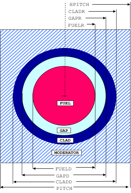
Fig. 7.1.1 Arrangement of materials in a SQUAREPITCH and SPHSQUAREP unit cell.
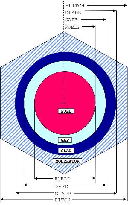
Fig. 7.1.2 Arrangement of materials in a TRIANGPITCH and SPHTRIANGP unit cell.
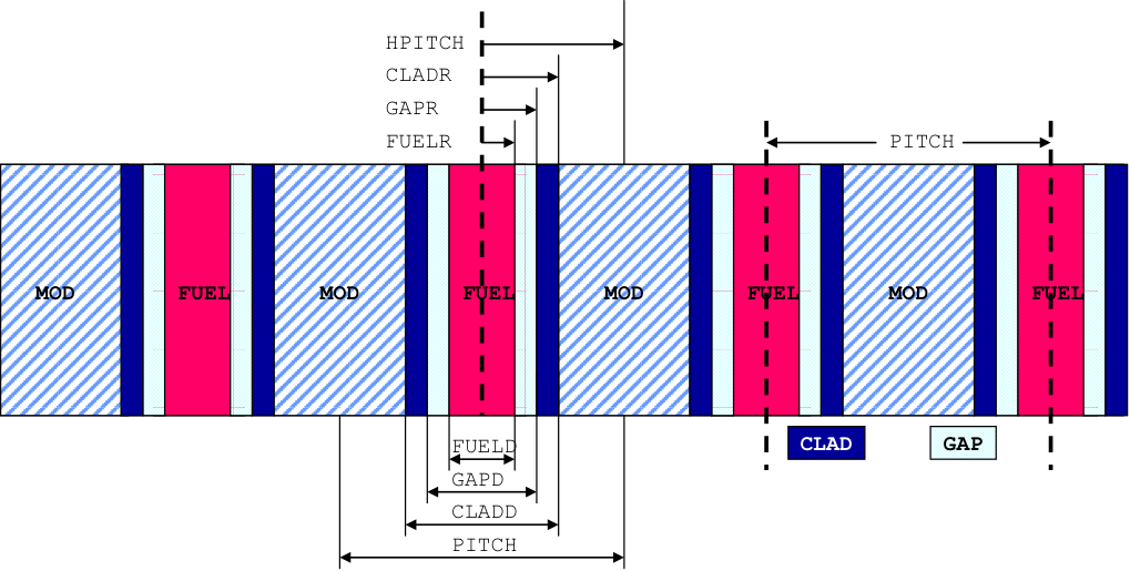
Fig. 7.1.3 Arrangement of materials in a SYMMSLABCELL unit cell having reflected left and right boundary conditions.
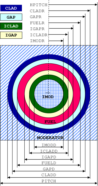
Fig. 7.1.4 Arrangement of materials in an ASQUAREPITCH and ASPHSQUAREP unit cell.
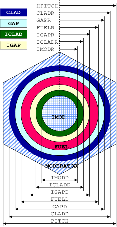
Fig. 7.1.5 Arrangement of materials in an ATRIANGPITCH and ASPHTRIANGP unit cell.
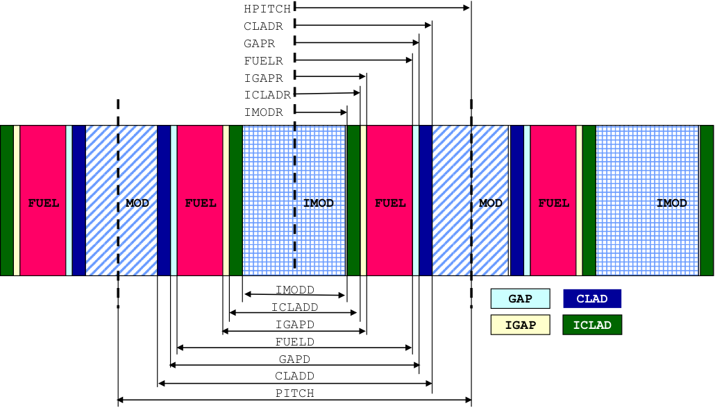
Fig. 7.1.6 Arrangement of materials in an ASYMSLABCELL unit cell having reflected left and right boundary conditions.
7.1.3.6. Unit cell specification for MULTIREGION cells
A MULTIREGION cell can be used to define a 1-D geometric arrangement that is more general than allowed by a LATTICECELL. It can also be used for large geometric regions where the geometry effects for the cross sections are small. For CENTRM/PMC self-shielding, lattice effects can be approximated by applying reflected, periodic, or white external boundary conditions to a MULTIREGION cell. HOWEVER, MULTIREGION CELLS SHOULD NOT BE USED FOR BONAMI-ONLY SELF-SHIELDING OF AN ARRAY UNIT CELL. In this case a LATTICECELL should always be used for BONAMI self-shielding in order to incorporate the proper Dancoff effects.
The data required for a MULTIREGION cell are given in Table 7.1.9 and explained in the following text.
celltype
MULTIREGION. The keyword MULTIREGION is used to represent arbitrary 1-D geometries, with no restrictions the on number or placement of mixtures in the cell. The keyword may be truncated to any number of characters as long as the characters presented are identical from the beginning of the keyword (i.e., M is acceptable).
cs
TYPE OF GEOMETRY. The type of geometry must always be specified for a MULTIREGION cell. The available geometry options are listed below.
SLAB. This is used to describe a slab geometry.
CYLINDRICAL. This is used to describe cylindrical geometry.
SPHERICAL. This is used to describe spherical geometry.
BUCKLEDSLAB. This is used for slab geometry with a buckling correction for the two transverse directions. Inactive in SCALE 6.2 and later.
BUCKLEDCYL. This is used for cylindrical geometry with a buckling correction in the axial direction. Inactive in SCALE 6.2 and later.
RIGHT_BDY
RIGHT BOUNDARY CONDITION. This is defaulted to VACUUM. The available options and their qualifications are listed below.
VACUUM. This imposes a vacuum at the boundary of the system.
REFLECTED. This imposes mirror image reflection at the boundary. Do not use for CYLINDRICAL or SPHERICAL.
PERIODIC. This imposes periodic reflection at the boundary. Do not use for CYLINDRICAL or SPHERICAL.
WHITE. This imposes isotropic return at the boundary.
LEFT_BDY
LEFT BOUNDARY CONDITION. This is defaulted to REFLECTED. The available options and their qualifications are listed below.
VACUUM. This imposes a vacuum at the boundary of the system.
REFLECTED. This imposes mirror image reflection at the boundary. For CYLINDRICAL or SPHERICAL, this is the only valid boundary condition because the left boundary corresponds to the centerline of the cylinder or the center of the sphere.
PERIODIC. This imposes periodic reflection at the boundary.
WHITE. This imposes isotropic return at the boundary.
ORIGIN
LOCATION OF LEFT BOUNDARY ON THE ORIGIN. The default value of ORIGIN is 0.0. This is the only value allowed for CYLINDRICAL or SPHERICAL geometry. For SLABs, enter the location of the left boundary on the X-axis perpendicular to the slab (in cm).
DY
BUCKLING HEIGHT. This is the buckling height in cm. It corresponds to one of the transverse dimensions of an actual 3-D slab assembly or the length of a finite cylinder. Inactive in SCALE 6.2 and later.
DZ
BUCKLING DEPTH. This is the buckling width in cm. It corresponds to the second transverse dimension of an actual 3-D slab assembly. Inactive in SCALE 6.2 and later.
CELLMIX
CELL-WEIGHTED MIXTURE NUMBER. Enter ONLY if a cell-weighted mixture is required. Enter a unique mixture number used to create a cell-weighted homogeneous mixture (Sect. 7.1.2.4).
END
The word END is entered to terminate these data before entering the zone description data. It must not be entered in columns 1 through 3, and at least two blanks must separate it from the zone description. A label can be associated with this END. The label can be a maximum of 12 characters and is separated from the END by a single blank. At least two blanks must follow this entry.
The zone description data are entered at this point. Entries 10 and 11 are entered for each zone, and the sequence is repeated until all the desired zones have been described. To terminate the data, enter the words END ZONE. Zone dimensions must be in increasing order.
mxz
MIXTURE NUMBER IN THE ZONE. Enter the mixture number of the material that is present in the zone. Enter a zero for a void. Repeat the sequence of entries 10 and 11 for each zone. Mixtures other than zero must not be used more than once in a cell and may be used in no more than one cell.
rz
OUTSIDE RADIUS OF THE ZONE. Enter the outside dimension of the zone in cm.
In SLAB geometry, rz is the location of the zone’s right boundary on the X-axis. Repeat the sequence of entries 10 and 11 for each zone.
END ZONE
Is used to terminate the MULTIREGION zone data. Enter the words END ZONE when all the zones have been described. Note that ZONE is a label associated with this END. This label can be as long as 12 characters, but the first four characters must be ZONE. At least two blanks must follow this entry.

|
7.1.3.7. Unit cell specification for doubly heterogeneous (DOUBLEHET) cells
The data required for a DOUBLEHET cell are given in Table 7.1.10 and explained in the following text.
Details about the computation procedures for DOUBLEHET cells can be found in Sect. 7.1.2.3.
“Grain” refers to a spherical fuel particle surrounded by one or more coating zones and does not include the matrix material the grains are in. “Grain type” refers to a grain that has specified dimensions and mixtures such as a 0.025-cm-radius UO2 fuel kernel with a 0.01-cm-thick carbon coating. Another grain type could be a 0.012-cm-radius PuO2 fuel kernel with a 0.01-cm-thick carbon coating. The user must first define all grain types in a fuel element. Next, all fuel element–related data must be entered.
Since all grains and the matrix material are homogenized into a single uniform mixture for the fuel element, there are restrictions on how each grain type must be defined so that the volume fraction of each grain type within the homogenized fuel mixture can be determined. Related entries are PITCH, NUMPAR (number of particles), and VF (volume fraction). If there is only one grain type for a fuel element, the code needs the pitch and will directly use the input value if entered. If PITCH is not given, then the VF (if given) is used to calculate the pitch. If neither PITCH nor VF is given, then NUMPAR is used to calculate the pitch and the volume fraction. The user should only enter one of these items.
If more than one grain type is present, additional information is needed since all grain types are homogenized into a single mixture. Similar to the one grain type case, the pitch is needed to perform the CENTRM spherical cell calculations. However, the pitch by itself is not sufficient to perform the homogenization. Therefore, the user needs to input VF or NUMPAR for each grain type. Since each grain’s volume is known (grain dimensions must always be entered), entering NUMPAR or VF for each grain type essentially provides the total volume of each grain type and therefore enables the calculation of the other unknowns (VF or NUMPAR, and PITCH). In this case, since pitch is not given, the available matrix material is distributed around the grains of each grain type proportional to the grain volume to calculate the corresponding pitch.
Syntax:
DOUBLEHET fuelmix END
GF(D|R)=fuel mg (COAT(D|R)=coat mc)|(COATT=coat mc) {H}PITCH=mod MATRIX=mm NUMPAR=npar VF=vf END GRAIN
mct ctp FUEL(D|R)=mfuel {FUELH=hfuel} {FUELW=wfuel} {GAP(D|R)=mgap mmg} {CLAD(D|R)=mclad mmc} {H}PITCH=mpitch mmm {CELLMIX=mcmx} END
celltype
DOUBLEHET. The keyword DOUBLEHET is used to represent a doubly heterogeneous problem such as fuel units that are composed of grains of fuel.
fuelmix
HOMOGENIZED MIXTURE NUMBER. Enter a unique mixture number to be used for the homogenized grains and matrix material.
END
The word END is entered to terminate these data before entering the grain and fuel element description data. It must not be entered in columns 1 through 3, and at least two blanks must separate it from the zone description. A label can be associated with this END. The label can be a maximum of 12 characters and is separated from the END by a single blank. At least two blanks must follow this entry.
The grain description data are entered at this point. Entries 5 through 12 are entered for each grain, and the sequence is repeated until all the grains have been described. To terminate the data, enter the words END GRAIN. Data may be entered in any order.
PITCH or HPITCH
EQUIVALENT CELL DIMENSION. This is the equivalent spherical diameter (or radius), in cm, of the “average” unit cell for this grain, as shown in Fig. 7.1.7. Physically, the volume of the average unit cell is equal to the volume of the fuel element divided by the total number of all grain types.
GFD or GFR
OUTSIDE DIMENSION OF FUEL. This is the outside diameter or radius of the fuel zone in a grain, fuel, in cm followed by the fuel mixture number, mg, as shown in Fig. 7.1.7.
COATD or COATR
OUTSIDE DIMENSION OF COATING. This is the outside diameter or radius of a coating zone, coat, in cm followed by the coating mixture number, mc, as shown in Fig. 7.1.7. As many coating-mixture pairs as desired may be entered. If the coating dimensions are entered using COATD or COATR, then the COATT keyword should not be used.
COATT
THICKNESS OF COATING. This is the thickness of a coating zone, coat, in cm followed by the coating mixture number, mc, as shown in :numref`fig7-1-7`. As many coating-mixture pairs as desired may be entered. If the coating dimensions are entered using COATT, then the COATD or COATR keyword should not be used.
MATRIX
MIXTURE NUMBER OF THE MATRIX MATERIAL. This is the mixture number, mm, of the matrix material that encloses the grains.
NUMPAR
NUMBER OF PARTICLES. This is the number of grains, npar, of this type in each fuel element.
VF
VOLUME FRACTION. This is the volume fraction, vf, of grains of this type in each fuel element’s fuel zone. A fuel element’s fuel zone is entered using the entry number 16-FUELD (or FUELR).
END GRAIN
This is used to terminate the grain zone data for this grain type. At least two blanks must follow this entry.
REPEAT ENTRIES 4-11 FOR EACH GRAIN TYPE IN A FUEL ELEMENT.
mct
TYPE OF FUEL ELEMENT (macro cell type). One of the keywords PEBBLE or ROD or SLAB is entered to indicate the type of the fuel element, i.e., the second layer of heterogeneity. This data must be entered. The keyword may NOT be truncated. PEBBLE is used for spherical fuel elements; ROD is used for cylindrical fuel elements; and SLAB for plate fuel elements.
ctp
TYPE OF LATTICE. This defines the type of lattice or array configuration. Any one of the following alphanumeric descriptions may be used. Note that the alphanumeric description must be separated from subsequent data entries by one or more blanks. Fig. 7.1.1 Mixture and position data are entered using keywords. Mixture number 0 may be entered for void and may be used multiple times in each and all unit cells. For regular cells, the minimum requirement is that a fuel region and a moderator region are specified and no inner components are specified. For annular cells, the minimum requirement is the fuel and outer moderator and inner moderator regions are specified. Regular and annular cell configurations are specified as shown below.
Regular Cells
SQUAREPITCH is used for an array of cylinders arranged in a square lattice, as shown in Fig. 7.1.1. The clad and/or gap can be omitted.
TRIANGPITCH is used for an array of cylinders arranged in a triangular-pitch lattice as shown in Fig. 7.1.2. The clad and/or gap can be omitted.
SPHSQUAREP is used for an array of spheres arranged in a square-pitch lattice. A cross section view through a cell is represented by Fig. 7.1.1. The clad and/or gap can be omitted.
SPHTRIANGP is used for an array of spheres arranged in a triangular-pitch (dodecahedral) lattice. A cross section view through a cell is represented by Fig. 7.1.2. The clad and/or gap can be omitted.
SYMMSLABCELL is used for an infinite array of symmetric slab cells, as shown in Fig. 7.1.3. The clad and/or gap can be omitted.
Annular Cells
ASQUAREPITCH or ASQP is used for annular cylindrical rods in a square-pitch lattice as shown in Fig. 7.1.4. The inner and outer clad and gap are independently entered so they may be different materials and dimensions.
ATRIANGPITCH or ATRP is used for annular cylindrical rods in a triangular-pitch lattice as shown in Fig. 7.1.5. The inner and outer clad and gap are independently entered, so they may be different materials and dimensions.
ASPHSQUAREP or ASSP is used for spherical shells in a square-pitch lattice as shown in Fig. 7.1.4. The inner and outer clad and gap are independently entered, so they may be different materials and dimensions.
ASPHTRIANGP or ASTP is used for spherical shells in a triangular-pitch (dodecahedral) lattice as shown in Fig. 7.1.5. The inner and outer clad and gap are independently entered, so they may be different materials and dimensions.
ASYMSLABCELL is used for a periodic, but asymmetric, array of slabs as shown in Fig. 7.1.6. The inner and outer clad and gap are independently entered, so they may be different materials and dimensions.
PITCH or HPITCH
ARRAY PITCH. This is the center-to-center spacing or half-spacing between the fuel lumps (pebbles or rods or slabs), mpitch, in cm followed by the outer moderator material number, mmm, as shown in Fig. 7.1.1 and Fig. 7.1.2.
FUELD or FUELR
OUTSIDE DIMENSION OF FUEL. This is the outside dimension (diameter or radius for sphere/cylinder or x-thickness for slab) of the fuel region, mfuel, in cm, as shown in Fig. 7.1.1 and Fig. 7.1.2.
FUELH
HEIGHT OF FUEL ROD OR SLAB. This is the height (z-dimension) of the fuel plate, hfuel, in cm. (only used to compute volume of fuel plate).
FUELW
WIDTH OF FUEL ROD or slab. This is the width/depth (y-dimension) of the fuel plate, wfuel, in cm. (only used to compute volume of fuel plate).
GAPD or GAPR
OUTSIDE DIMENSION OF GAP. Enter only if outer gap is present. This is the outside diameter or radius of the outer gap, mgap, in cm followed by the gap mixture number, mmg, as shown in Fig. 7.1.1 and Fig. 7.1.2.
CLADD or CLADR
OUTSIDE DIMENSION OF CLAD. Enter ONLY if a clad is present. This is the outside diameter or radius of the outer clad, mclad, in cm followed by the clad mixture number, mmc, as shown in Fig. 7.1.1 and Fig. 7.1.2.
CELLMIX
CELL-WEIGHTED MIXTURE NUMBER. Enter ONLY if cell-weighted mixture, mcmx, is to be created.
IMODD or IMODR
DIMENSION OF INNER MODERATOR. Enter ONLY if an annular cell is specified. This is the outside diameter or radius of the inner moderator, imod, in cm followed by the inner moderator mixture number, mim, as shown in Fig. 7.1.4 through Fig. 7.1.6.
IGAPD or IGAPR
OUTSIDE DIMENSION OF INNER GAP. Enter ONLY if an annular cell is specified and inner gap is present. This is the outside diameter or radius of the inner gap, igap, in cm followed by the inner gap mixture number, mig, as shown in Fig. 7.1.4 through Fig. 7.1.6.
ICLADD or ICLADR
OUTSIDE DIMENSION OF INNER CLAD. Enter ONLY if an annular cell is specified and inner clad is present. This is the outside diameter or radius of the inner clad, iclad, in cm followed by the inner clad mixture number, mic, as shown in Fig. 7.1.4 through Fig. 7.1.6.
END
The word END is entered to terminate the DOUBLEHET data. An optional label can be associated with this END. The label can be as many as 12 characters long and is separated from the END by a single blank. At least two blanks must follow this entry.
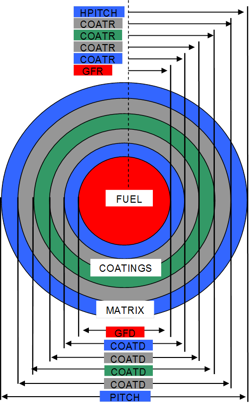
Fig. 7.1.7 Arrangement of materials in a grain (first level cell) in a DOUBLEHET unit cell.

|

|

|
7.1.3.8. Optional MORE DATA parameter data
MORE DATA is an optional sub-block of the READ CELL block. MORE DATA parameters allow certain default options in BONAMI and XSDRNPM to be modified for individual cell calculations. Each MORE DATA sub-block applies only to the unit cell immediately preceding it. However a MORE DATA sub-block placed prior to all unit cell definitions applies to all mixtures not assigned to a unit cell, which are treated as infinite homogeneous media. If the default parameters are acceptable, this section of input data should be omitted in its entirety. Non-default values for one or more of the parameters can be specified by entering the words MORE DATA followed by the desired keyword parameters and their associated values. One or more of the parameters can be entered in any order. Default values are used for parameters that are not entered. Each parameter is entered by spelling its name, followed immediately by an equal sign and the value to be entered. There should not be a blank between the parameter name and the equal sign. Each parameter specification must be separated from the rest by at least one blank. For example, if an XSDRNPM calculation is performed for particular unit cell (e.g., cellmix= is specified),
MORE DATA ISN=16 EPS=0.00008 END MORE
would result in using an S16 angular quadrature set and tightening the convergence criteria to 0.00008 in the XSDRNPM calculation.
A description of each entry is given. (Also see sections on BONAMI and XSDRNPM input description.)
MORE DATA These words, followed by one or more blanks, are entered ONLY if optional parameter data are to be entered. Entries 2 through 42 can be entered in any order.
NSENSX This is the XSDRNPM sensitivity output file for TSUNAMI sequences.
CROSSEDT BONAMI CROSS SECTION EDIT. Cross section print option for BONAMI 0/1 –no/yes (default is 0).
FFACTEDT BONDARENKO FACTOR EDIT. Bondarenko factor (f-factor) print option 0/1 –no/yes (default is 0).
ISSOPT BONAMI BACKGROUND XSEC OPTIONS. BONAMI background cross section selection option if > 1000 potential; otherwise, total cross section is used (default is –1).
IROPT BONAMI IR/NR CALCULATION OPTION. BONAMI uses intermediate resonance (IR) if iropt=1 and narrow resonance (NR) approximation for iropt=0 (default is 0).
BELLOPT BELL FACTOR OPTION. Optional user-defined bell factor calculation option (default is -1).
BELLFACT BELL FACTOR. Optional user-defined bell factor for BONAMI (default is 0.0).
ESCXSOPT ESCAPE CROSS SECTION CALC OPTION. Escape cross section calculation for IR calculations. 0/1 =consistent/inconsis tent (default is 0).
BONAMIEPS BONAMI CONVERGENCE CRITERIA. BONAMI Bondarenko iteration convergence criteria (default is 0.001).
LBARIN INPUT MEAN CORD LENGTH. Mean cord length for each zone (default is 0.00).
ADJTHERM ADJUST 1D THERMAL CROSS SECTIONS TO MATCH SUM OF 2D CROSS SECTIONS. Flag determining whether 1-D cross sections are scaled to match the 2-D cross sections or the 2-D cross sections are scaled to match the 1-D cross sections.
EXSIG ESCAPE CROSS SECTION. External escape cross section for BONAMI (default is 0.00).
IEVT XSDRNPM CALCULATION TYPE. The type of calculation to be performed- fixed source, eigenvalue, alpha, zone width search, outer radius search, buckling search, direct buckling search (default is 1).
ICLC THEORY OPTION. Number of outer iterations to use an alternative theory (diffusion, infinite medium, or BN) before using discrete ordinates. Negative values indicate alternative theory (default is 0).
IPVT PARAMETRIC EIGENVALUE SEARCH. 0 – none; 1 – search for eigenvalue equal PV; 2 – alpha search (default is 0).
IPP WEIGHTED CROSS SECTION PRINT. 2 -> No print; -1 -> 1-D edit; 0-N – edit through PN cross section arrays (default is 2).
IFLU GENERALIZED ADJOINT CALCULATION. 0 is a standard calculation; 1 is a generalized adjoint calculation (default is 0).
IFSN FISSION SOURCE SUPPRESSION. Non-zero suppresses the fission source in a fixed source calculation (default is 0).
IQM VOLUMETRIC FIXED SOURCES. The number of volumetric sources in a fixed source problem (default is 0).
IPM BOUNDARY FIXED SOURCES. The number of boundary sources in a fixed source problem (default is 0).
XNF SOURCE NORMALIZATION FACTOR. The value used to normalize the problem source (default is 1.0).
VSC VOID STREAMING CORRECTION. The height of a void streaming path in a cylinder or slab in centimeters (default is 0.0).
EV EIGENVALUE GUESS. Starting eigenvalue guess for a search calculation (default is 0.0).
EQL INITIAL SEARCH CONVERGENCE. Initial eigenvalue search convergence (default is 0.0001).
XNPM DAMPING FACTOR. Damping factor used in search calculations (default is 0.75).
ISN ORDER OF ANGULAR QUADRATURE FOR XSDRNPM. Quadrature sets are geometry-dependent quantities that are defaulted to order 8 by the XSProc for LATTICECELL and cylindrical MULTIREGION. The default is 32 for MULTIREGION slabs and spheres. See the automatic quadrature generator and Appendix B for a more detailed explanation.
SZF SPATIAL MESH SIZE FACTOR FOR XSDRNPM. The size of the mesh intervals can be adjusted by entering a value for SZF, which is a multiplier of the mesh size. The default value is 1.0. A value between zero and 1.0 yields a finer mesh; a value greater than 1.0 yields a coarser mesh. If SZF \(\leq 0\), the user specifies the number of mesh intervals in each zone immediately following the MORE DATA block. If SZF = 0, the interval spacing is automatically generated, while if SZF < 0 the intervals are equally spaced intervals in each zone.
IIM MAXIMUM NUMBER OF INNER ITERATIONS FOR XSDRNPM. This is the maximum number of inner iterations to be used in the XSDRNPM calculation. The default value is 20. See Appendix B for a more detailed explanation.
ICM MAXIMUM NUMBER OF OUTER ITERATIONS FOR XSDRNPM. This is the maximum number of outer iterations to be used in the XSDRNPM calculation. The default value is 25. If the calculation reaches the outer iteration limit, a larger value should be used. See Appendix B for a more detailed explanation.
EPS OVERALL CONVERGENCE CRITERIA FOR XSDRNPM. This is used by XSDRNPM after each outer iteration to determine if the problem has converged. The default value of EPS is 0.00001. A value less than 0.00001 tightens the convergence criteria; a larger value loosens the convergence criteria.
PTC POINTWISE CONVERGENCE CRITERIA FOR XSDRNPM. This is the point flux convergence criteria used by XSDRNPM to determine if convergence has been achieved after an inner iteration. The default value for PTC is 0.000001. A smaller value tightens convergence; a larger value loosens it.
BKL BUCKLING FACTOR FOR XSDRNPM. A buckling factor should be used ONLY for a MULTIREGION BUCKLEDSLAB or BUCKLEDCYL problem. Because cylinders are assumed to be infinitely long and slabs are assumed to be infinite in both transverse directions, the analytic sequence may tend to overestimate the total flux for a finite system. A buckling correction can be used to approximate the leakage from the system in the transverse direction(s). The extrapolation distance factor, BKL, is defaulted to 1.420892.
IUS UPSCATTER SCALING FLAG for XSDRNPM. This option allows the use of upscatter scaling to accelerate the solution or force convergence. The default value is zero, in which case upscatter scaling is not used. IUS=1 facilitates upscatter scaling. Guidelines are not available to indicate when upscatter scaling is needed. Some problems will not converge with it, and some will not converge without it. See Appendix B for a more detailed explanation.
DAN(mm) DANCOFF FACTOR for the specified mixtures used in BONAMI and in the CENTRM 2REGION option. This value overrides the internally computed Dancoff factor used in the resonance correction for the specified mixture mm. The Dancoff data are entered in the form DAN(mm) = Dancoff factor. Note that the parentheses must be entered as part of the data, and the mixture number, mm, must be enclosed in the parentheses. See Appendix B for additional details. (Note: this is not to be confused with the DAN2PITCH parameter in CENTRMDATA)
BAL BALANCE TABLE PRINT FLAG for XSDRNPM. This allows control of the balance table print from XSDRNPM. The default value is FINE. BAL=NONE suppresses the balance table print. BAL=ALL prints all of the balance tables. BAL=FINE prints only the fine-group balance tables. See Appendix B for additional details.
DY FIRST TRANSVERSE DIMENSION for XSDRNPM. This is the first transverse dimension, in cm, used in a buckling correction to calculate the leakage normal to the principal calculation direction (the height of a slab or cylinder). It should only be entered if XSDRNPM is to create cell-weighted cross sections and/or calculate the eigenvalue of a cylinder or slab system of finite height for a LATTICECELL problem. DY= is defaulted to an infinite height, or is set to DY for a buckled MULTIREGION cell description. A value entered here overrides any buckling height value entered in the MULTIREGION data.
DZ SECOND TRANSVERSE DIMENSION for XSDRNPM. This is the second transverse dimension, in cm, used for a buckling correction for a slab of finite width. It should only be entered if XSDRNPM is to create cell-weighted cross sections and/or calculate the eigenvalue of a LATTICECELL slab of finite width. DZ= is defaulted to an infinite width, or is set to DZ for a buckled MULTIREGION slab cell of finite width. A value entered here overrides any buckling depth value entered in the MULTIREGION data.
COF DIFFUSION COEFFICIENT FOR TRANSVERSE LEAKAGE CORRECTIONS IN XSDRNPM. The default value is 3. The available options are as follows.
COF=0 sets a transport-corrected cross section for each zone
COF=1 use a spatially averaged diffusion coefficient for each zone
COF=2 use a diffusion coefficient for all zones that is one-third of the diffusion coefficient determined from the spatially averaged transport cross section for all zones
COF=3 use a flux and volume weighting across all zones
See Appendix B or XSDRNPM Input/Output Assignments in the XSDRNPM chapter, 3$ array, variable IPN for more details.
NT3 UNIT WHERE XSDRNPM WRITES THE WEIGHTED LIBRARY. If XSDRN does a weighting calculation, this is the unit number it uses to write the weighted library on (default is 3).
NT4 UNIT WHERE XSDRNPM WRITES THE ANGULAR FLUXES. XSDRN writes the angular fluxes on this unit if it is non-zero (default is 16).
ADJ Adjoint mode flag for XSDRNPM. Set to 1 to cause XSDRNPM to solve the adjoint problem (default is 0).
NTA UNIT WHERE XSDRNPM WRITES THE ACTIVITIES. XSDRN writes the calculated activities on this unit if it is non-zero (default is 75).
NBU UNIT WHERE XSDRNPM WRITES BALANCE TABLES. If the balance tables file is to be saved, enter the unit number where it is to be written (default is 76).
NTC UNIT WHERE XSDRNPM WRITES THE DERIVED DATA. XSDRN writes the derived input data on this unit if it is non-zero (default is 73).
NTD UNIT WHERE XSDRNPM WRITES THE DATA FOR A SENSITIVITY ANALYSIS. XSDRN writes the data for a sensitivity analysis on this unit if it is non-zero (default is 0).
FRD UNIT WHERE XSDRNPM READS INPUT FLUX GUESS. If greater than 0, a flux guess will be read from this unit.
FWR UNIT WHERE XSDRNPM WRITES OUPUT FLUX. If greater than 0, the space-dependent multigroup scalar flux is written in binary format to this unit.
WGT CROSS SECTION WEIGHTING FLAG for XSDRNPM. The default is 0, not to perform cross section weighting. To turn on cross section weighting, a positive value should be entered. A value of 1 will weight the cross sections by nuclide; 2 will weight by mixture.
ZMD(iz) ZONE WIDTH MODIFIERs for an XSDRNPM search problem. This allows entering a zone width modifier for zone iz in the XSDRNPM problem description. The zone width data are entered in the following form:
ZMD(iz)=modifier
Note that the parentheses must be entered as part of the keyword. The zone number iz, to which the modifier is applied, must be enclosed in the parentheses. The modifier is entered after the equal sign. See the “Dimension Search Calculations” description in the XSDRNPM chapter for more information.
INT(iz) NUMBER OF MESH INTERVALS FOR ZONE IZ in XSDRNPM. The default is 0, which causes the number to be calculated. The data are entered in the following form:
INT(iz)=number
Note that the parentheses must be entered as part of the keyword. The zone number iz, for which the number of intervals is specified, must be enclosed in the parentheses. The number of intervals is entered after the equal sign.
KEF DESIRED VALUE OF kEFF for an XSDRNPM zone width search. The default value is 1.0. If it is desired to search for some other value, such as 0.9, then input it here.
KFM The first eigenvalue modifier used in an XSDRNPM search. This value is used to make the first change in the XSDRNPM search. The default value is -0.1. A user may sometimes need to change this to make the search converge.
ID1 SCALAR FLUX PRINT CONTROL. The default value is -1, which suppresses printing the scalar fluxes in XSDRNPM. See the XSDRNPM Input/Output Assignments section in the XSDRNPM chapter, 2$ array, variable ID1 for allowed values and corresponding actions.
ISCT ORDER OF SCATTERING for XSDRMPM. The default is 5 for all libraries.
ICON TYPE OF WEIGHTING (see Cross-Section Weighting section in the XSDRNPM chapter).
INNERCELL - followed by integer N (zones in the cell). Cell weighting is performed over the N innermost regions in the problem. Nuclides outside these regions are not weighted.
CELL - cell weighting
ZONE - zone weighting
REGION - region weighting
IGMF NUMBER OF GROUPS IN COLLAPSED LIBRARY. Enter number of groups after equal sign, followed by group lower energy boundaries (eV) in descending order.
ITP COLLAPSED OUTPUT FORMAT. The default is 0.
0-19 - cross sections are written only in the AMPX weighted library formats on logical 3. A weighted library is always written when IFG=1.
The various values of ITP (modulo 10) are used to select the different transport cross section weighting options mentioned earlier. The options are as follows:
ITP = 0, 10, … \(\sqrt{(\psi^{g}_{1} + (DG\psi))^{2}}\)
ITP = 1 ,11, … absolute value of current
ITP = 2, 12, … \(DB^{2}\psi_{g}\) + outside leakage
ITP = 3, 13, … \(\frac{\psi}{\Sigma^{g}_{t}}\)
ITP = 4, 14, … \(DB\psi_{g}\)
ITP = Other values are reserved for future development and should not be used.
GAMMA_MT_LIST LIST OF GAMMA 1D REACTIONS ASSOCIATED WITH INPUT. A list of 1-D gamma reactions to be included on a condensed library for later use gamma_mt_list= numberEntries mt1 mt2 … mt_numberEntries.
NEUTRON_MT_LIST LIST OF NEUTRON 1D REACTIONS ASSOCIATED WITH INPUT. A list of 1-D neutron reactions to be included on a condensed library for later use neutron_mt_list= numberEntries mt1 mt2 … mt_numberEntries.
NEUTRON_2D_LIST LIST OF NEUTRON 2D ARRAYS FOR THE MICRO LIBRARY. This list flags the finalizer to place 2-D arrays (currently MT 2, 4, 16) on the micro library for use in SAMS.
ACTIVITY Enter:
IAZ (number of activities)
IAI (calculate activities by zone or interval)
0 – zone
1 – interval
LACFX (unit number to which activities are written)
LAZ (IAZ sets of numbers consisting of the nuclide and process numbers for each activity)
BAND NUMBER OF REBALANCE BANDS for XSDRNPM (default is 1).
IPRT CROSS SECTION PRINT CONTROL. The default value is -2, which suppresses printing the cross sections in XSDRNPM. See XSDRNPM chapter, 2$ array, variable IPRT for allowed value, and corresponding actions.
GRAIN_K Flag to control execution of XSDRNPM after each grain calculation for a DOUBLEHET cell.
SOURCE(iz) ZONE SOURCE for an XSDRNPM fixed source problem. This allows entering a source spectrum for zone iz in the XSDRNPM problem description. The source spectrum data are entered in the following form:
SOURCE(iz)= numEntries spectrum_grp_1 … spectrum_grp_numEntries
Note that the parentheses must be entered as part of the keyword. The zone number, iz, to which the spectrum is applied, must be enclosed by the parentheses. The numEntries follows the equal sign and must be less than or equal to the number of energy groups for the problem. It is followed by numEntries numbers defining the spectrum for the first numEntries groups for zone iz. Groups not defined are set to zero. The spectrum applies uniformly to zone iz. A different spectrum may be entered for different zones.
END MORE Terminate the optional parameter data.
7.1.3.9. Optional CENTRM DATA parameter data
The CENTRM DATA block defines input parameter values for the CENTRM, PMC and CRAWDAD modules. XSProc defines default values for these parameters which are adequate for most applications. If all default values are acceptable, this section of input data can be omitted. The CENTRM DATA block applies only to the unit cell immediately preceding it. CENTRM DATA placed prior to all unit cell data applies to all materials not listed in any unit cell. Parameter values are assigned by entering the words CENTRM DATA followed by the desired keyword parameters and their associated values. One or more parameters can be entered in any order. There should not be a blank between the parameter name and the equal sign. Each parameter specification must be separated from the rest by at least one blank. For example,
CENTRM DATA ISN=16 PTC=0.0008 N1D=1 END CENTRM DATA
A description of CENTRM DATA parameters is given below.
CENTRM DATA These words, followed by one or more blanks, are entered ONLY if optional parameter data are to be entered. They must precede all other optional parameter data. Entries 2 through 42 can be entered in any order.
ISN ORDER OF SN ANGULAR QUADRATURE FOR CENTRM. SN Quadrature sets are geometry-dependent quantities. Default value for ISN is 6 (only used for NFST and NTHR=0; and NPXS=1).
ISCT LEGENDRE POLYNOMIAL PN ORDER OF SCATTERING. These are used to determine the number of moments calculated for the scattering cross sections. Default value is 0 for 2-D MoC option and 1 for 1-D Sn, which have been found adequate for nearly all cases.
IIM MAXIMUM NUMBER OF INNER ITERATIONS. This is the maximum number of inner iterations for Sn transport calculations in CENTRM. Default value is 10.
IUP MAXIMUM NUMBER OF OUTER ITERATIONS IN THERMAL RANGE. This is the maximum number of outer iterations used to converge PW flux changes caused by upscattering in the thermal range. Default value is 3. More iterations (~ 15) may be required for higher accuracy in some cases.
NFST FAST RANGE MULTIGROUP CALCULATION OPTION, E > DEMAX. This determines what type of calculation is done above DEMAX. The options are (0) S:sub:N, (1) diffusion theory, (2) homogenized infinite medium, (3) zonewise infinite medium, or (6) 2D MoC lattice cell [NOTE: NFST=4,5 are deprecated]. Default value is 0 (SN).
NTHR THERMAL RANGE MULTIGROUP CALCULATION OPTION, E < DEMIN. This determines what type of calculation is done below DEMIN. The options include (0) S:sub:N, (1) diffusion, (2) homogenized infinite medium, (3) zonewise infinite medium, or (6) 2-D MoC lattice cell [NOTE: NTHR=4,5 are deprecated]. Default value is 0 (SN ).
NPXS POINTWISE RANGE MULTIGROUP CALCULATION OPTION, DEMIN < E < DEMAX. This determines what type of calculation is done between DEMIN and DEMAX. The options include (0) MG calculation, (1) 1-D SN, (2) collision probability, (3) homogenized infinite medium, (4) zonewise infinite medium, (5) two-region, or (6) 2-D MoC lattice cell. Default value is 1 (SN), except for square-pitch LATTICECELL where the default is 6 (2D MoC).
ISVAR LINEARIZATION OPTION. This determines if the MG source and/or the cross sections are linearized in CENTRM calculations. Options for linearizing are (0) neither, (1) source, (2) cross section, or (3) both. Default value is 3.
ISCTI LEGENDRE POLYNOMIAL PN ORDER OF SCATTERING IN THE INELASTIC RANGE. These are used to determine the number of moments calculated for the inelastic scattering cross sections. Default value is 0, isotropic.
NMF6 INELASTIC FLAG. This determines if inelastic data are used. The options are to include (-1) no inelastic data, (0) discrete inelastic data, and (1) discrete inelastic and continuum. Default value is -1. Use of NMF6=1 is not recommended due to long running times.
IPRT MIXTURE CROSS-SECTION OUTPUT OPTION. This determines the output of cross section. The options include (-3) none, (-2) output macro PW cross sections to file “_centrm.pw.macroxs”, (-1) 1-D MG cross sections, (N) P0 to PN MG 2-D matrices. Default value is -3, none.
ID1 FLUX EDIT OPTION. This option determines the output of flux energy spectra. The options are (-1) none, (0) print MG fluxes, (1) also print MG flux moments, (2) save CE fluxes on output file, “_centrm.pw_flux”. Default value is -1.
KERNEL BOUND KERNELS. This indicates use of CENTRM PW thermal kernel data [S(\(\alpha\),:math:beta)] for bound nuclides if KERNEL=1. If KERNEL=0, all thermal kernels are treated as free gas; Default is 1, use bound scattering kernels if available.
IPBT PRINT GROUP SUMMARY TABLES. Group summary tables for each zone are printed in CENTRM if greater than 0. Default is 0. Balance ratios are not computed in thermal groups or for MoC option.
IPN GROUP DIFFUSION COEFFICENT. Used for DB2 loss term. See XSDRNPM chapter for more information. Default is 2.
IXPRT PRINT OPTION FOR CENTRM. This value is >0 if more information is printed to output. Default value is 0, minimum output.
MLIM MASS VALUE RESTRICTION ON ORDER OF SCATTERING. Nuclides with mass ratios greater than MLIM are limited to a NLIM order of scattering. Default value is 100.
NLIM ORDER OF SCATTERING RESTRICTION. This is the limiting order of scattering for all nuclides with mass ratios greater than MLIM. Default value is 0.
EPS INTEGRAL CONVERGENCE CRITERIA. This is used by CENTRM after each outer iteration to determine if the problem has converged. Default value is 0.001. A value less than 0.0001 tightens the convergence criteria; a larger value loosens the convergence criteria.
PTC POINTWISE CONVERGENCE CRITERIA. This is the point flux convergence criteria used by CENTRM to determine if convergence has been achieved after an inner iteration. Default value is 0.0001. A smaller value tightens convergence; a larger value loosens it.
B2 MATERIAL BUCKLING FACTOR (cm-2). This is used with a buckled system. If a buckled system is specified for a unit cell, the code will use this value. Default value is 0.0.
DEMIN LOWEST ENERGY OF POINTWISE FLUX CALCULATION. This value is the lowest energy (eV) for which CENTRM calculates PW fluxes. Default is 0.001 eV.
DEMAX HIGHEST ENERGY OF POINTWISE FLUX CALCULATION. This value is the highest energy (eV) for which CENTRM calculates PW fluxes. Default is 20,000.0 eV, which encompasses the resolved resonance range of all actinides. It is recommended that DEMAX be <500 keV.
TOLE CENTRM PW THINNING TOLERANCE. This is the tolerance used to thin the PW material cross sections after they are mixed. Default value is 0.001.
FLET FRACTIONAL LETHARGY CONSTRAINT. This is the maximum lethargy difference between points in the flux solution energy mesh. Smaller values increase the number of energy points. Default value is 0.1.
DAN2PITCH CENTRM DANCOFF FACTOR SEARCH. Fuel Dancoff factor to search for a Dancoff-equivalent pitch used in the CENTRM cell calculation. Only applicable in LATTICECELL and DOUBLEHET cases with fuel in center region, with SN or MoC transport solvers. Default is 0, which indicates no pitch modification. NOTE! This option should not be used to enter Dancoff factors for the CENTRM 2REGION transport option-use EDAN(m) array in MOREDATA for these values.
MRANGE PMC GROUP CROSS-SECTION PROCESSING RANGE. This option determines the range over which the group cross sections will be processed. The options are (0) compute new group cross section over the PW range, (1) over the resolved resonance range of each nuclide, or (2) over the PW flux range (DEMAX to DEMIN). Default value is 2.
N2D PMC ELASTIC MATRIX PROCESSING FLAG. This option determines how MG PN elastic scattering matrices are obtained. Options are (-2) perform operations in both (-1) and (2); (-1) compute P0 self-scatter, then renormalize matrix to shielded 1-D elastic values; (0) normalize original scatter matrix to shielded 1-D elastic values; (1) compute new PN moments of elastic matrix using scalar flux and S-wave kinematics for both thermal and epithermal energy ranges; or (2) use flux-moments to compute “consistent PN” correction for diagonal elements of elastic PN components. Default value is -1. For unit cell calculations in reactor lattices, option -2 may improve results. NOTE: option 0 is always used in thermal range except for option 1.
IXTR3 PMC PN ORDER FLAG. This option determines the maximum order of Legendre moments to be retained on output MG library. The default is 5; i.e., retain scattering moments up to P5 if available on the input MG library. If (-1) is entered, all elastic moments on the MG library are included.
NPRT PMC PRINT FLAG. This option determines what is printed to output. The options include (-1) minimum output, (0) standard output, (1) print 1-D cross sections, (2) print both 1-D and 2-D cross sections. Default value is -1, minimum output.
NWT PMC MULTIGROUP SPATIAL-WEIGHTING FLAG. This option determines if the MG data are (0) zone-weighted or (1) cell-weighted. Default value is 0.
MTT PMC MT PROCESSING FLAG. This option determines if reaction MTs are processed individually or treat dependencies explicitly. If MTT=0 all MTs are processed independently; if MTT=1, all MTs are processed except 1, 27, and 101. These are then computed as follows: MT101 = sum MT102 - 114, MT27 = MT18 + MT101, MT1 = MT2 + MT4 + MT16 + MT17 + MT27. Default value is 1.
N1D PMC WEIGHTING FUNCTION FLAG. This is used to determine if (0) flux weighting or (1) current weighting is used to collapse the cross sections. Default value is 0, flux weighting.
PMC_DILUTE PMC DILUTE BACKGROUND CROSS SECTION. The background cross section \(\sigma_{0}\) value above which nuclide cross sections are not processed in PMC but the BONAMI cross sections are used instead. No resonance shielding corrections are performed for materials with background cross sections greater than pmc_dilute. Higher values of pmc_dilute result in more nuclides being processed. The default value is 1.0E10.
MTOUT PW REACTION TYPES. Reactions included by CRAWDAD on PW library for MG processing in PMC: (0) all; (1) output only MTs 1, 2, 4, 102, 18, 452, 455, 456 (and 107 for 10B or 7Li); (2) all from option (1) and all inelastic MTs and 16. Default is MTOUT=1 for NMF6=-1 and MTOUT=2 for NMF6>-1.
IBR CENTRM RIGHT BOUNDARY TYPE. Type of boundary condition on right boundary of unit cell for CENTRM LATTICECELL calculations. See allowable IBR values in CENTRM. Default is white (IBR = 3) for 1D SN; 2D MoC transport option always uses reflected.
IBL CENTRM LEFT BOUNDARY TYPE. Same as IBR, but for left boundary. Default is reflected (IBL = 1).
ALUMP MASS LUMPING FRACTION. A value in range [0.0, 1.0] indicates fractional mass lumping criterion for CENTRM. Value of 0 indicates no lumping applied. For example, ALUMP=0.3 means that materials are combined into one or more lumps such that their masses are within +/-30% of the effective lump mass, while preserving the slowing-down power. This approximation reduces execution time. Default value is 0.2.
PMC_OMIT PMC NUCLIDES SKIPPED. PMC normally processes problem-dependent (e.g., self-shielded) MG cross sections for all materials. If PMC_OMIT=1, processing is only performed for materials contained in fuel mixtures. Default value is 0 (all materials processed).
PXSMEM CENTRM PW DATA STORAGE. Option to store PW data in memory or in external file during centrm execution. If PXSMEM=1, PW cross section data are stored by group in external scratch file during CENTRM calculation; if PXSMEM=0 (default value), all PW cross sections are kept in memory.
MOCMESH CENTRM MOC MESH OPTION. Pre-defined space mesh intervals for CENTRM MoC calculation: 0=>coarse mesh (1 interval per zone); 1=>regular mesh (4 intervals in fuel, 2 in moderator, 1 in others); 2=> fine mesh (8 in fuel, 4 in moderator, 1 in others). Default=0.
MOCRAY CENTRM MOC RAY SPACING. Distance between characteristic rays in CENTRM MoC calculation. Default=0.02.
MOCPOL CENTRM NUMBER OF MOC POLAR ANGLES. Allowable values are 2, 3, 4. Default=3 (only used for NPXS=6).
MOCAZI CENTRM NUMBER OF MOC AZIMUTHAL ANGLES. Allowable values are 2–16. Default=8 (only used for NPXS=6).
MOCZONE_INT CENTRM MOC MESH BY ZONE. User-defined mesh intervals by zone; e.g., moczone_int(1)=5 defines five intervals for zone 1; zero value means not used. This overrides the predefined meshs described by MOCMESH
ISRC CENTRM SOURCE TYPE. CENTRM can use a fission-spectrum source (isrc=1), an input source spectrum (isrc=0), or a combination(isrc=3) for transport. Default=1.
XNF CENTRM SOURCE NORMALIZATION. The integrated source (fission-spectrum and/or fixed source spectrum) is normalized to this value. Default=1.0.
ITERP CRAWDAD TEMPERATURE INTERPOLATION METHOD. Method to use for CE cross section interpolation 0=>combination of square-root(T) and finite-difference; 1=>only square-root(T); 2=> only finite-difference. Default is 0.
END CENTRM The word END is entered to terminate the optional parameter data. A label can be associated with this END. The label can be as long as 12 characters but must be preceded by a single blank. If this END is entered without a label, it must not begin in column 1. At least two blanks must follow this entry.
References
- XSProc-IB64
Igor Ilich Bondarenko. Group constants for nuclear reactor calculations. Consultants Bureau, 1964.
- XSProc-RLL+15
Bradley T. Rearden, Robert A. Lefebvre, Jordan P. Lefebvre, Kevin T. Clarno, Mark A. Williams, Lester M. Petrie, and Ugur Mertyurek. Modernization enhancements in SCALE 6.2. In PHYSOR 2014. Kyoto, Japan, 2015.
- XSProc-Wil11(1,2)
Mark L. Williams. Resonance self-shielding methodologies in SCALE 6. Nuclear Technology, 174(2):149–168, May 2011. URL: https://doi.org/10.13182/NT09-104, doi:10.13182/NT09-104.
- XSProc-WA95
Mark L. Williams and Mehdi Asgari. Computation of continuous-energy neutron spectra with discrete ordinates transport theory. Nuclear Science and Engineering, 121(2):173–201, 1995. Publisher: Taylor & Francis.
7.1.4. Appendices
- 7.1.4.1. XSProc: Standard Composition Examples
- 7.1.4.1.1. Standard composition fundamentals
- 7.1.4.1.2. Basic standard composition specifications
- 7.1.4.1.3. User-defined (arbitrary) chemical compound specifications
- 7.1.4.1.4. User-defined (arbitrary) mixture/alloy specifications
- 7.1.4.1.5. Fissile solution specifications
- 7.1.4.1.6. Combinations of standard composition materials to define a mixture
- 7.1.4.1.7. Combinations of user-defined compound and user-defined mixture/alloy to define a mixture
- 7.1.4.1.8. Combinations of solutions to define a mixture
- 7.1.4.1.9. Combinations of basic and user-defined standard compositions to define a mixture
- 7.1.4.1.10. Combinations of basic and solution standard compositions to define a mixture
- 7.1.4.1.11. Combinations of user-defined compound and solution to define a mixture
- 7.1.4.2. XSProc Standard Composition Examples
- 7.1.4.3. Examples of Complete XSProc Input Data
- 7.1.4.3.1. Infinite homogeneous medium input data
- 7.1.4.3.2. LATTICECELL input data
- 7.1.4.3.3. MULTIREGION input data
- 7.1.4.3.4. DOUBLEHET input data
- 7.1.4.3.5. Two methods of specifying a fissile solution
- 7.1.4.3.6. Multiple unit cells in a single problem
- 7.1.4.3.7. Multiple fissile mixtures in a single unit cell
- 7.1.4.3.8. Cell weighting an infinite homogeneous problem
- 7.1.4.3.9. Cell weighting a LATTICECELL problem
- 7.1.4.3.10. Cell weighting a MULTIREGION problem