2.1. CSAS: Control Module For Enhanced Criticality Safety Analysis Sequences With KENO
K. B. Bekar, L. M. Petrie 1, S. Goluoglu 1, D. F. Hollenbach 1 and N. F. Landers 1
The Criticality Safety Analysis Sequences with KENO codes provide reliable and efficient means of performing keff calculations for systems that are routinely encountered in engineering practice. Two CSAS sequence implementations, CSAS5 and CSAS6, with two variants of KENO codes, KENO V.a and KENO-VI, provide identical solution capabilities with different geometry packages. In the multigroup calculation mode, CSAS uses XSProc to process the cross sections for temperature corrections and problem-dependent resonance self-shielding and calculates the keff of a three-dimensional (3D) system model. If the continuous-energy calculation mode is selected no resonance processing is needed and the continuous-energy cross sections are used directly in KENO codes, with temperature corrections provided as the cross sections are loaded. The geometric modeling capabilities available in KENO codes coupled with the automated cross-section processing within the control sequences allow complex, 3D systems to be easily analyzed.
The CSAS5 search capability available in previous SCALE versions is no longer supported by the CSAS5 sequence in SCALE 6.3.
In SCALE 6.3, CSAS5 and CSAS6 support two new sequence data blocks, definitions and tallies data, to allow flexible definition and output control of mesh tallies. The mesh responses neutron flux, fission rate, and fission source can now be requested multiple times on different spatial and energy grids in the same calculation.
1 Formerly with Oak Ridge National Laboratory.
2.1.1. Acknowledgments
CSAS5 and its related Criticality Safety Analysis sequences are based on the old CSAS2 control module (no longer in SCALE) and the KENO V.a functional module described in Sect. 8.1. Therefore, special acknowledgment is made to J. A. Bucholz, R. M. Westfall, and J. R. Knight who developed CSAS2. G. E. Whitesides is acknowledged for his contributions through early versions of KENO. Appreciation is expressed to C. V. Parks and S. M. Bowman for their guidance in developing CSAS5.
2.1.2. Introduction
Criticality Safety Analysis Sequence with KENO V.a (CSAS5) and KENO-VI (CSAS6) provide reliable and efficient means of performing keff calculations for systems that are routinely encountered in engineering practice, especially in the calculation of keff of three-dimensional (3D) system models. CSAS5 and CSAS6 implement XSProc to process material input and provide a temperature and resonance-corrected cross-section library based on the physical characteristics of the problem being analyzed. If a continuous energy cross-section library is specified, no resonance processing is needed and the continuous energy cross sections are used directly in KENO codes, with temperature corrections provided as the cross sections are loaded.
The search capability available in the CSAS5S in previous SCALE versions is no longer supported by the CSAS5 in SCALE 6.3. This capability was excluded when doing modernization work for CSAS sequences in SCALE 6.2 and permanently disabled in SCALE 6.3 due to the inconsistencies between the legacy code implementation and the modern CSAS framework. Research is being continued to support equivalent search capabilities in a more robust modernized code framework for the next SCALE release.
In SCALE 6.3, CSAS5 and CSAS6 support two new sequence data blocks, definitions and tallies data, to allow flexible definition and output control of mesh tallies. The mesh responses neutron flux, fission rate, and fission source can now be requested multiple times on different spatial and energy grids in the same calculation. This capability helps users efficiently manage computational resources when collecting detailed information, depending on their requirements. For example, fission density can be tallied in a very fine spatial mesh in a few energy groups while performing calculations in high resolution with SCALE’s very fine group multigroup library (1597 energy groups), or fission density can be tallied on multiple spatial fine meshes rather than using a large global fine mesh to keep the runtime and memory footprint of the calculation at reasonable levels.
2.1.3. Sequence Capabilities
In the CSAS sequence framework, SCALE data handling is automated as much as possible. CSAS and many other SCALE sequences apply a standardized procedure to provide appropriate number densities and cross sections for the calculation. XSProc is responsible for reading the standard composition data and other engineering-type specifications, including volume fraction or percent theoretical density, temperature, and isotopic distribution as well as the unit cell data. XSProc then generates number densities and related information, prepares geometry data for resonance self-shielding and flux-weighting cell calculations, if needed, and (if needed) provides problem-dependent multigroup cross-section processing. Sequences that execute KENO codes include a KENO Data Processor to read and check the KENO data. When the data checking has been completed, the control sequence executes XSProc to prepare a resonance-corrected microscopic cross-section library in the AMPX working library format if a multigroup library has been selected.
For each unit cell specified as being cell-weighted, XSProc performs the necessary calculations and produces a cell-weighted microscopic cross-section library. KENO codes may be executed to calculate the keff or neutron multiplication factor using the cross-section library that was prepared by the control sequence.
Computational capabilities available in KENO codes—including the determination of k-effective, neutron lifetime, generation time, energy-dependent leakages, energy- and region-dependent absorptions, fissions, the system mean-free-path, the region-dependent mean-free-path, average neutron energy, flux densities, fission densities, reaction rate tallies, mesh tallies, source convergence diagnostics, problem-dependent continuous-energy temperature treatments, parallel calculations, restart capabilities, and many more—are also provided by the CSAS5 sequence. Details of each capability, their input methods, and output edits are provided in Sect. 8.1 of this document and will not be repeated here.
2.1.3.1. Multigroup limitations
The CSAS control module was developed to use simple input data and prepare problem-dependent cross sections for use in calculating the effective neutron multiplication factor of a 3D system using KENO codes, KENO V.a and KENO-VI. An attempt was made to make the system as general as possible within the constraints of the standardized methods chosen to be used in SCALE. Standardized methods of data input were adopted to allow easy data entry and for quality assurance purposes. Some of the limitations of the CSAS multigroup sequences are a result of using preprocessed multigroup cross sections. Inherent limitations in multigroup CSAS calculations are as follows:
1. Two-dimensional (2D) effects such as fuel rods in assemblies where some positions are filled with control rod guide tubes, burnable poison rods and/or fuel rods of different enrichments. The cross sections are processed as if the rods are in an infinite lattice of identical rods. If the user inputs a Dancoff factor for the cell (such as one computed by MCDancoff), XSProc can produce an infinite lattice cell, which reproduces that Dancoff. This can mitigate some two dimensional lattice effects
2.1.3.2. Continuous energy limitations
When continuous energy KENO calculations are desired, none of the resonance processing capabilities of XSProc are applicable or needed. The continuous energy cross sections are directly used in KENO. An existing multigroup input file can easily be converted to a continuous energy input file by simply specifying the continuous energy library. In this case, all cell data is ignored. However, the following limitations exist:
If CELLMIX is defined in the cell data, the problem will not run in the continuous energy mode. CELLMIX implies new mixture cross sections are generated using XSDRNPM-calculated cell fluxes and therefore is not applicable in the continuous energy mode.
Only VACUUM, MIRROR, PERIODIC, and WHITE boundary conditions are allowed. Material-specific albedos, e.g., WATER, CARBON, POLY, etc., are for multigroup only.
Problems with DOUBLEHET cell data are not allowed as they inherently utilize CELLMIX feature.
2.1.4. Input Data Guide
This section describes the input data required for the CSAS with
KENO transport codes. A typical CSAS input,
shown in Example 2.1.1, starts
with the sequence identifier always preceded by the = sign
(=CSAS5 and =CSAS6), and
it is followed by the problem title. Then, a cross section library
name is specified, and all these entries are followed by several
data blocks each starting with READ data_block and
ending with END data_block.
=sequence_identifier parm=(parm_options)
problem title

' ----- XSProc data
' cross section library name (REQUIRED)
ce_v7.1

' List of material specifications in standard SCALE format (REQUIRED)
read composition
...
end composition

' Specify data for resonance processing (OPTIONAL)
read celldata
...
end celldata

' ---- New CSAS sequence data blocks

' Used to define energy bounds and grid geometries for
' the tallies defined in tallies data block
' (REQUIRED if tallies data block exists)
read definitions
...
end definitions

' Used to define tallies in a more robust way (OPTIONAL)
read tallies
...
end tallies

' ---- KENO transport data
' Specify the problem geometry (REQUIRED)
read geometry
...
end geometry

' Other input data blocks (OPTIONAL)
The input data for the CSAS sequence are composed of three broad categories of data, as shown in Example 2.1.1. The first is XSProc data, including Standard Composition Specification Data and Unit Cell Geometry Specification Data. This first category specifies the cross section library and then defines the composition of each mixture and optionally unit cell geometry that may be used to process the cross sections. This data block is necessary for the CSAS sequence.
Note
Sequence implementation determines the calculation (transport) mode automatically, either as multigroup or continuous-energy, by testing the cross section library whose name has been entered.
Warning
Continuous-energy mode does not process data entered in celldata data block(s).
The second category of data, the CSAS sequence input data, includes
two new data blocks, definitions data and tallies data, for
flexible tally definitions. These new blocks available in all CSAS
sequences in SCALE 6.3 currently provide only accumulation of neutron
flux, fission rate, and neutrons produced from fission on
different energy and spatial grids. Although similar to capabilities
activated with old-style KENO parameter input methods (with GFX,
CDS, and FIS as described in Sect. 8.1.3.3), these input
methods do not allow tallying the requested quantities on different
energy and spatial grids. This limitation is relaxed with the new
CSAS input blocks.
The third category of data, the KENO input data, is used to specify the geometric and boundary conditions that represent the physical 3D configuration of a KENO problem.
CSAS ensures data consistency among these three category of data.
For example, it verifies that mixture numbers used in the KENO
geometry data block must correspond to those defined
either in the composition data or celldata data blocks.
Note that in multigroup mode, a unique mixture number can be
specified in the celldata data block by CELLMIX=
if the cell is cell-weighted.
Note
As depicted in Example 2.1.1, a successful CSAS calculation requires at least a problem title and cross section library definitions, followed by composition data and geometry data. Depending on the requirements of the problem, other optional data blocks can be activated. Following CSAS5 input demonstrates this minimal requirement.
=csas5
sample problem 14  u metal cylinder in an annulus
ce_v7.1

read comp
   uranium  1 den=18.69 1 300  92235 93.2 92238 5.6 92234 1.0 92236 0.2 end
end comp

read geom
   global unit 1
      cylinder  1 1 8.89 10.109 0.0 orig 5.0799 0.0
      cylinder  0 1 13.97 10.109 0.0
      cylinder  1 1 19.05 10.109 0.0
end geom
end data
end
Unlike the CSAS5 and CSAS6 versions in previous SCALE releases, in SCALE 6.3, user can enter all data blocks in any order in both CSAS5 and CSAS6 inputs. Following CSAS5 input illustrates this input flexibility.
=csas5
sample problem 14  u metal cylinder in an annulus
ce_v7.1

read geom
   global unit 1
      cylinder  1 1 8.89 10.109 0.0 orig 5.0799 0.0
      cylinder  0 1 13.97 10.109 0.0
      cylinder  1 1 19.05 10.109 0.0
end geom

read comp
   uranium  1 den=18.69 1 300  92235 93.2 92238 5.6 92234 1.0 92236 0.2 end
end comp

end data
end
All data are entered in free form, allowing alphanumeric data, floating-point data, and integer data to be entered in an unstructured manner. Up to 252 columns of data entry per line are allowed. Data can usually start or end in any column with a few exceptions. As an example, the word END beginning in column 1 and followed by two blank spaces or a new line will end the problem and any data following will be ignored. Each data entry must be followed by one or more blanks to terminate the data entry. For numeric data, either a comma or a blank can be used to terminate each data entry. Integers may be entered for floating-point values. For example, 10 will be interpreted as 10.0. Imbedded blanks are not allowed within a data entry unless an E precedes a single blank as in an unsigned exponent in a floating-point number. For example, 1.0E 4 would be correctly interpreted as 1.0 \(\times\) 104.
The word “END” is a special data item. An “END” may have a name or label associated with it (e.g., “END DATA”). The name or label associated with an “END” is separated from the “END” by a single blank and is a maximum of 12 characters long. At least two blanks or a new line MUST follow every labeled and unlabeled ``END``. It is the user’s responsibility to ensure compliance with this restriction. Failure to observe this restriction can result in the use of incorrect or incomplete data without the benefit of warning or error messages.
Multiple entries of the same data value can be achieved by specifying
the number of times the data value is to be entered, followed by either
R, \*, or $, followed by the data value to be repeated. Imbedded blanks
are not allowed between the number of repeats and the repeat flag. For
example, 5R12, 5*12, 5$12, or 5R12, etc., will enter five successive
12’s in the input data. Multiple zeros can be specified as nZ where n is
the number of zeroes to be entered.
The purpose of this section is to define the input data in discrete subsections relating to a particular type of data. Tables of the input data are included in each subsection, and the entries are described in more detail in the appropriate sections.
Resonance-corrected cross sections are generated using the appropriate boundary conditions for the unit cell description (i.e., void for the outer surface of a single unit, white for the outer surface of an infinite array of cylinders). As many unit cells as needed may be specified in a problem. A unit cell is cell-weighted by using the keyword “CELLMIX=” followed by a unique user specified mixture number in the unit cell data.
To check the input data without actually processing the cross sections
and without performing transport calculations, the sequence parameter
options PARM=CHECK or PARM=CHK should be entered, as shown below.
=CSAS5 PARM=CHK

=CSAS6 PARM=CHK
This will cause the input data for CSAS to be checked and appropriate error messages to be printed. If plots are specified in the data, they will be printed. This feature allows the user to debug and verify the input data while using a minimum of computer time.
2.1.4.1. XSProc data
The XSProc reads the standard composition specification data and the unit cell geometry specifications. It then produces the mixing table and unit cell information necessary for processing the cross sections if needed. Sect. 7 of this manual provides a detailed description of the input data and processing options. CSAS sequences are responsible for passing data such that mixing table and problem-dependent cross sections from XSProc calculations are conveyed to the transport calculations. Note that reported elapsed time in each transport calculation does not include the time required to process and prepare multigroup cross section data. When running the transport module concurrently on multiple cores, these data are broadcasted to all instances of the transport module running on each computational node.
In contrast, in continuous-energy mode, only mixing table data generated from XSProc utilities are passed to the transport module. In addition to this, the defined continuous-energy data library is first verified by the utilities that exist in XSProc, and then temperature correction is applied to each nuclide data using the defined temperatures when loading these data from disk by each instance of the transport module. Therefore, elapsed time reported at the end of each transport module calculation also includes the time spent on temperature correction and data loading.
In multigroup mode, the XSProc calculation path for each unit cell is always determined with the following hierarchy to prepare the problem-dependent multigroup cross section data:
All non-fissionable cells are processed with BONAMI by default, and this cannot be changed.
All fissionable cells are processed with CENTRM by default, and this can be overridden by defining a cross section processing option with the sequence parameter option (PARM=BONAMI or PARM=2REGION).
Double-het cells defined in the celldata data block are always processed with CENTRM, and this cannot be changed.
CSAS sequences always print a cross section processing summary of the cells used/defined in the problem. This can be seen in Sect. 2.1.5.3. See Sect. 7 of this manual for detailed description of these unit cell processing options.
2.1.4.2. CSAS input data
Two new data blocks, definitions data and tallies data, are currently supported by CSAS sequences to provide flexible tally definitions. These new data blocks are currently available to define the mesh responses flux, fission_density, and fission_source on different spatial and energy grids. This section introduces these two new data blocks and discusses the limitations with some details.
2.1.4.2.1. Definitions data
The definitions data input block allows (1) multiple spatial grids to be defined using the gridGeometry data blocks inside the definitions data block, and (2) multiple energy grids to be defined using the energyBounds data inside the definitions data block. The syntax for defining a gridGeometry inside a definitions block is the same as defining a standalone grid at the root level of input (i.e., KENO’s gridgeometry data block). The syntax for defining energyBounds is already used for defining energy grids in the MAVRIC sequence. See Sect. 8.2 for further details.
The energy grid definition permits specification of individual energy boundaries, equal-width energy bins and equal-width lethargy bins within a specified energy, and SCALE energy group structures (such as the 56-group structure). The SCALE energy group structure can be any group structures that is used by a SCALE multigroup library that is available in the DATA directory. The syntax is <num>n for neutron libraries and <num>p for photon (gamma) libraries. A combination of the different options is also supported (see Example 2.1.2).
Note
As shown in example given Example 2.1.2
READ keyword is not required when defining energy boundaries with
energyBounds data block. This may show differences from one CSAS
sequence to another.
READ DEFINITIONS

read grid 1
   xlinear 30 -10 70
   ylinear 10 -20 60
   zlinear 50 -30 40
end grid

read grid 2
   numxcells=10 xmin=-18.5 xmax=+68.5
   numycells=25 ymin=-28.5 ymax=+58.5
   numzcells=10 zmin=-38.5 zmax=+48.5
end grid

'user specified energy grid
read energyBounds 1
   bounds 2e7 0.625 1e-5 end
end energyBounds

'user specified energy grid using equal-energy bins'
energyBounds 2
   linear=10 1e-5 2e7
end energyBounds

'user specified energy grid using equal-lethargy bins'
energyBounds 3
   logarithmic=10 1e-5 2e7
end energyBounds

'SCALE 56-group neutron structure with additional energy points'
energyBounds 10
   56n
   bounds 1.1  0.11 0.011 0.0011 end
energyBounds

END DEFINITIONS
In continuous-energy mode, a special DEFAULT keyword
allows modification of the default energy group structure
that was previously defined with the NGP parameter and/or
the KENO energy data block.
Note
The default energy group structure is currently
acquired from the SCALE 252-group neutron library. This may
be overridden by defining data with the NGP parameter,
data in the KENO energy data block, or data in
the definitions data block entered with DEFAULT keyword.
Caution
CSAS does not allow using definitions data block
together with KENO NGP parameter and/or KENO energy data
block.
Caution
CSAS does not allow using definitions data block
together with KENO FIS, GFX, CDS, and MSH parameters.
In multigroup mode, DEFAULT energy boundaries are always obtained from the multigroup library used by KENO codes in the neutron transport calculation, and this cannot be overriden by a DEFAULT energy boundaries specification in the definitions data block. In other words, an energyBounds DEFAULT is not permitted in multigroup mode.
Warning
In multigroup mode, DEFAULT energy boundaries are always acquired from the library used by the KENO V.a transport, and it cannot be changed.
Caution
In multigroup calculations, energy points of the user-defined energy boundaries must be a subset of the energy points of the energy structure obtained from the multigroup library used by KENO transport. Otherwise, execution will be terminated and an appropriate error message is displayed.
The sample definitions data block given in Example 2.1.3
defines an energy grid labeled 1 and an energy grid labeled DEFAULT
in the definitions data block.
 READ DEFINITIONS

 'user defined energy grid 1
   read energyBounds 1
      bounds 2e7 0.625 1e-5 end
   end energyBounds

 'user defined default energy grid
   energyBounds DEFAULT
      bounds    2e7 8.2e5 2.0e4 1.05e2 5.0 0.65 0.15 0.04 1.e-5 end
   end energyBounds

 END DEFINITIONS
When using this definitions block in
continuous-energy mode, KENO codes read DEFAULT energy boundaries from
the definitions data and utilizes these data in all tally
calculations (energyBounds DEFAULT overrides the current
default that is acquired from the SCALE 252-group library) if requested otherwise
in the tallies block for the supported mesh responses. The two
energy boundaries read from definitions data are printed
in KENO’s energy boundaries edit in the output as shown in
Fig. 2.1.1.
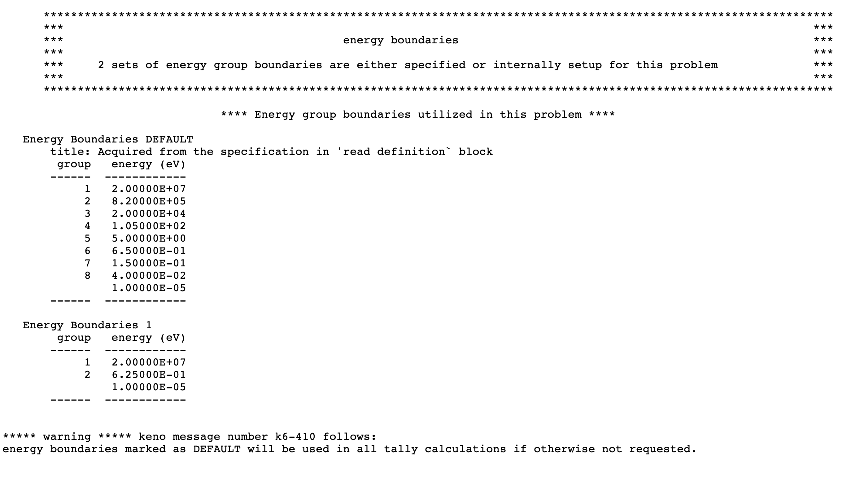
Fig. 2.1.1 Sample energy boundaries output edit when running CSAS with the above definitions data in the continuous-energy mode.
Unlike continuous-energy mode, when the data defined in
the sample definition block given above are processed in
mutigroup mode, reading the energy boundaries DEFAULT
from the definitions data is ignored, and the user is notified with a
warning message, as shown in Fig. 2.1.2.
However, the calculation is terminated because the
energy boundaries given with energy identifier 1 does
not conform to the default energy boundaries acquired from
the library used by KENO transport (in this test case,
the SCALE 28-group neutron and 19-group gamma library was used).
The corresponding error message is also shown in
Fig. 2.1.2 printed
to the output just before the code termination.
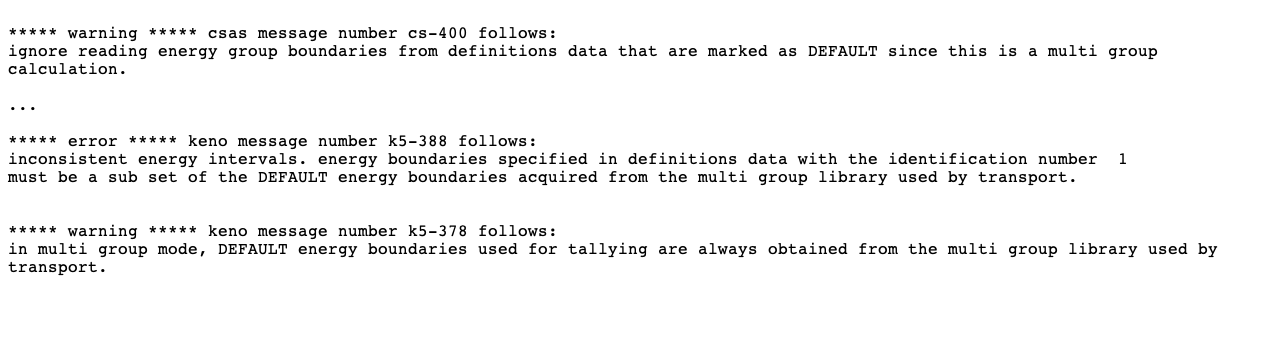
Fig. 2.1.2 CSAS terminates execution with an error message when the definitions data given above are used in multigroup mode.
2.1.4.2.2. Tallies data
The new tallies data input allows mesh responses to be
requested using any energy grid and/or spatial grid from
the definitions block. Three response types shown in
Table 2.1.1 were added as
mesh tally options for CSAS. Note that the same
responses can also be activated by GFX, FIS,
and CDS, but only using the default energy boundaries.
Description |
Old KENO input method to activate the same tally |
New response name in tallies implementation |
Neutron flux averaged over mesh volumes |
|
|
Fission rates per voxel volume |
|
|
Neutron production per voxel volume |
|
|
Note
Either input method (parameter input or tallies data)
can be used to request the mesh tallies described in Table 2.1.1.
It is recommended to request mesh tallies using the new response names (flux,
fission_density, fission_source) with the tallies data
block rather than the old-style parameter inputs (GFX, FIS, CDS)
with the limited energy and spatial grid options.
A typical mesh tally input block is given in Example 2.1.4. Each spatial and energy grid used by each mesh tally must be defined in the definitions data block. Note that, as shown in Example 2.1.4, the same mesh response can be defined multiple times using different spatial and energy grids.
READ TALLIES

   read mesh 1
      response=FLUX
      grid=1
      energy= 1
   end mesh

   read mesh 2
      response=FISSION_DENSITY
      grid=2
      energy=2
   end mesh

   read mesh 3
      response=FISSION_SOURCE
      grid=3
      energy=default
   end mesh

   read mesh 13
      response=FISSION_SOURCE
      grid=3
      energy=2
   end mesh

END TALLIES
The KENO codes in SCALE 6.3 support multiple sets of
energy group boundaries for tallying purposes. A data
container was designed to store all energy boundaries
that are either set up by KENO for some internal use
or specified by the user. Note that multiple
sets of energy boundaries can be defined only by
using the new definitions data block available in CSAS
and TRITON sequences. In continuous-energy mode,
KENO with the NGP parameter or data in energy
data block provides only a single set of energy boundaries, and
these always override KENO’s default energy group
boundaries used in all tallies.
After processing data entered in the definitions and tallies data blocks, KENO codes print the summary of all corresponding definitions in energy boundaries, grid definitions, and tally definitions output edits. The following sample input can be used to demonstrate the new output edits in KENO codes with continuous-energy mode:
read definitions

 read gridgeometry 11
    numxcells=2 numycells=2 numzcells=2
    xmin=-0.73 xmax=0.73
    ymin=-0.73 ymax=0.73
    zmin=0 zmax=10.0
 end gridgeometry

 read gridgeometry 12
    numxcells=2 numycells=2 numzcells=8
    xmin=-0.73 xmax=0.73
    ymin=-0.73 ymax=0.73
    zmin=0 zmax=10.0
 end gridgeometry

read gridgeometry 13
    numxcells=4 numycells=2 numzcells=4
    xmin=-0.73 xmax=0.73
    ymin=-0.73 ymax=0.73
    zmin=0 zmax=10.0
 end gridgeometry

 read energyBounds 12
   title "ebounds is a sub-set of 8 group MG test library"
   bounds
              2.00000E+07
              1.05000E+02
              5.00000E+00
              1.00000E-05
   end
 end energyBounds

 read energyBounds DEFAULT
   title "SCALE 8 group test library structure"
   bounds
             2.00000E+07
             8.20000E+05
             2.00000E+04
             1.05000E+02
             5.00000E+00
             6.50000E-01
             1.50000E-01
             4.00000E-02
             1.00000E-05
   end
 end energyBounds

end definitions

read tallies
read mesh 1
  energy=DEFAULT
  grid=11
  response=FLUX
end mesh

read mesh 2
  energy=DEFAULT
  grid=12
  response=FLUX
end mesh

read mesh 3
  energy=12
  grid=13
  response=FLUX
end mesh

read mesh 100
  energy=12
  grid=12
  response=FISSION_DENSITY
end mesh

read mesh 200
  energy=DEFAULT
  grid=13
  response=FISSION_DENSITY
end mesh

read mesh 1000
  energy=12
  grid=11
  response=FISSION_SOURCE
end mesh

read mesh 1080
  energy=DEFAULT
  grid=13
  response=FISSION_SOURCE
end mesh

end tallies
The energy boundaries output edit depicted in Fig. 2.1.3 summarizes the data stored in the energy boundaries data container. For the above sample problem, two sets of energy group boundaries are read from the definitions data and stored in the data container.
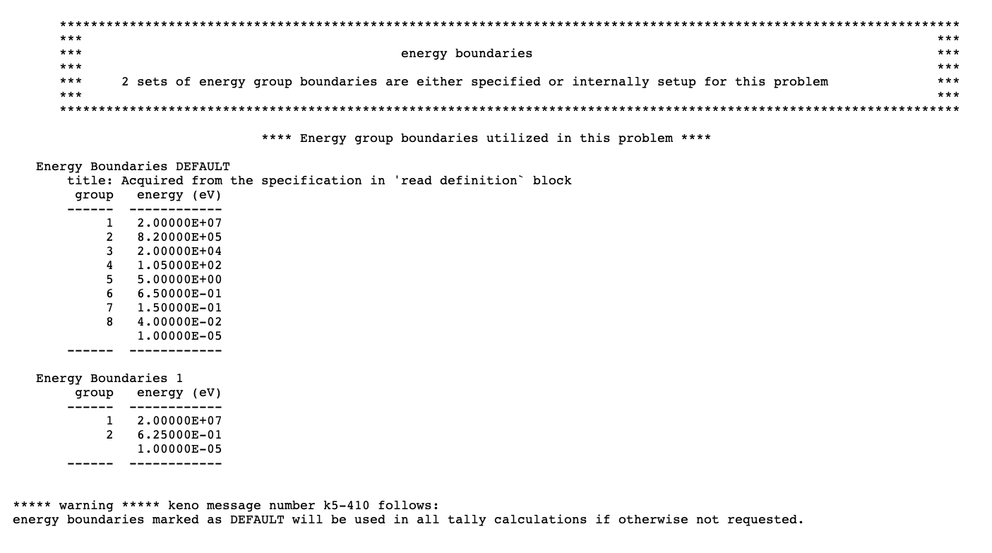
Fig. 2.1.3 Energy boundaries edit in KENO output
Another edit that was added to KENO’s output is the grid definitions edit, which summarizes the mesh grids that were either defined by the user or automatically constructed by KENO for Shannon entropy tallies. The grid definitions output edit corresponds to the above provided sample input and is shown in Fig. 2.1.4. Note that Fig. 2.1.4 shows only a part of the mesh tallies output edit.
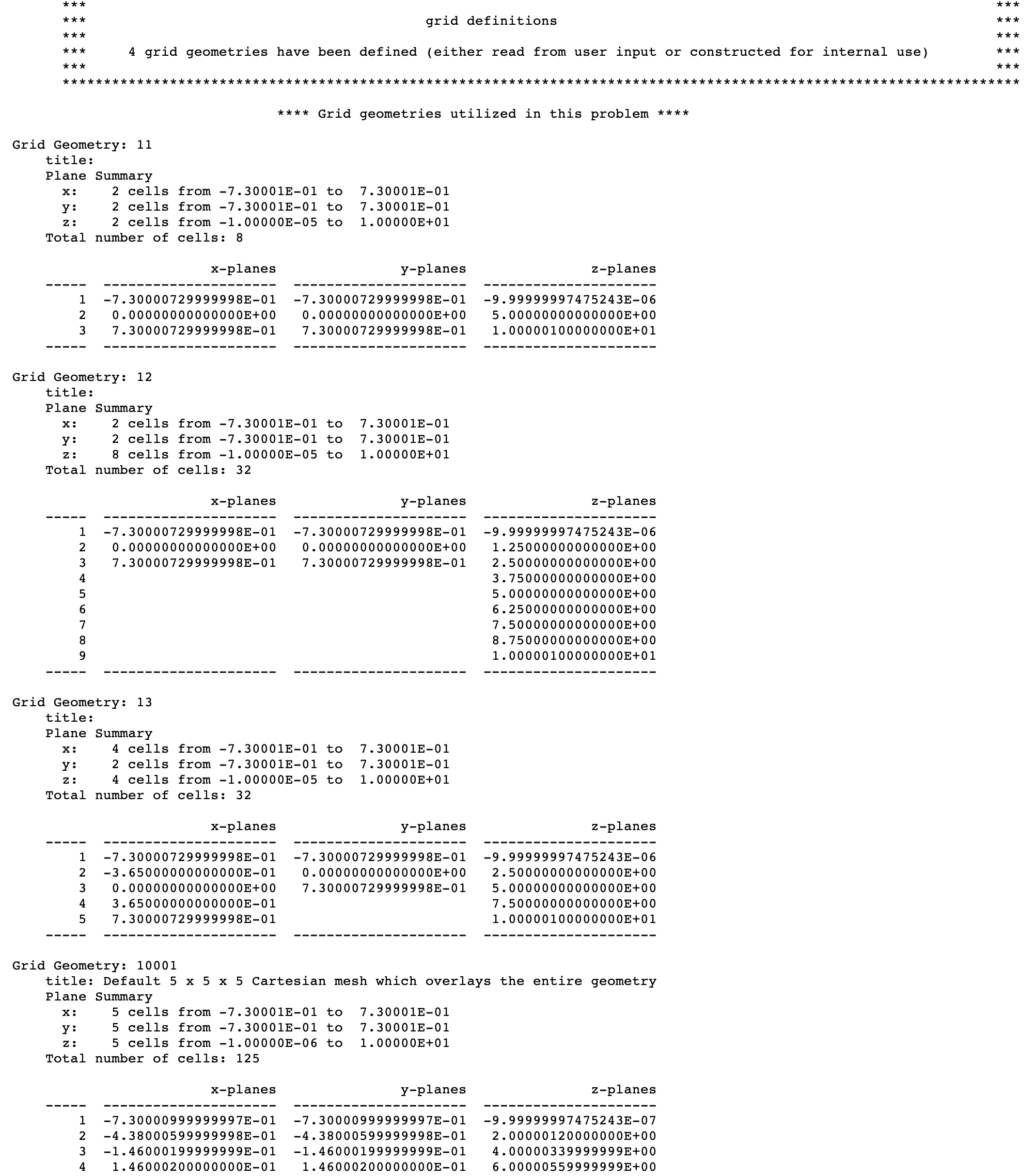
Fig. 2.1.4 Grid definitions edit in KENO output
The tally definitions output edit summarizes the specifications of tallies defined in tallies block. Currently, only mesh tally edits are supported, and this is shown in Fig. 2.1.5 for the above sample input.
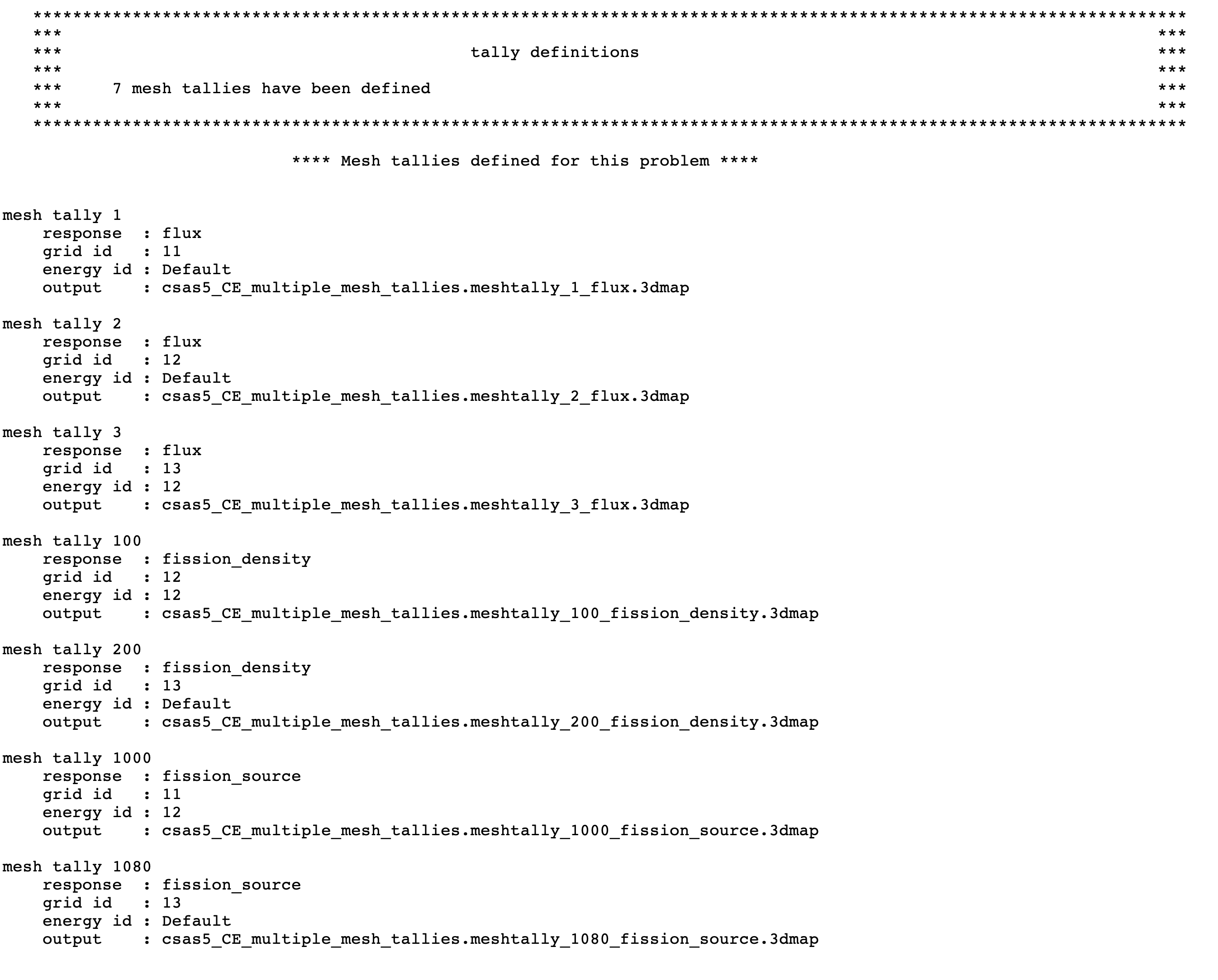
Fig. 2.1.5 Tally definitions edit in KENO output
After the calculations have been completed for all the requested tallies, KENO also prints another output table that summarizes the mesh tallies, as shown in Fig. 2.1.6. Other than the mesh tally input specifications, the mesh tallies output edit also summarizes the intervals of the energy and spatial grids used in tally calculations and approximate memory allocation required to compute and write this tally to 3dmap output file. Note that Fig. 2.1.6 shows only a part of the mesh tallies output edit.
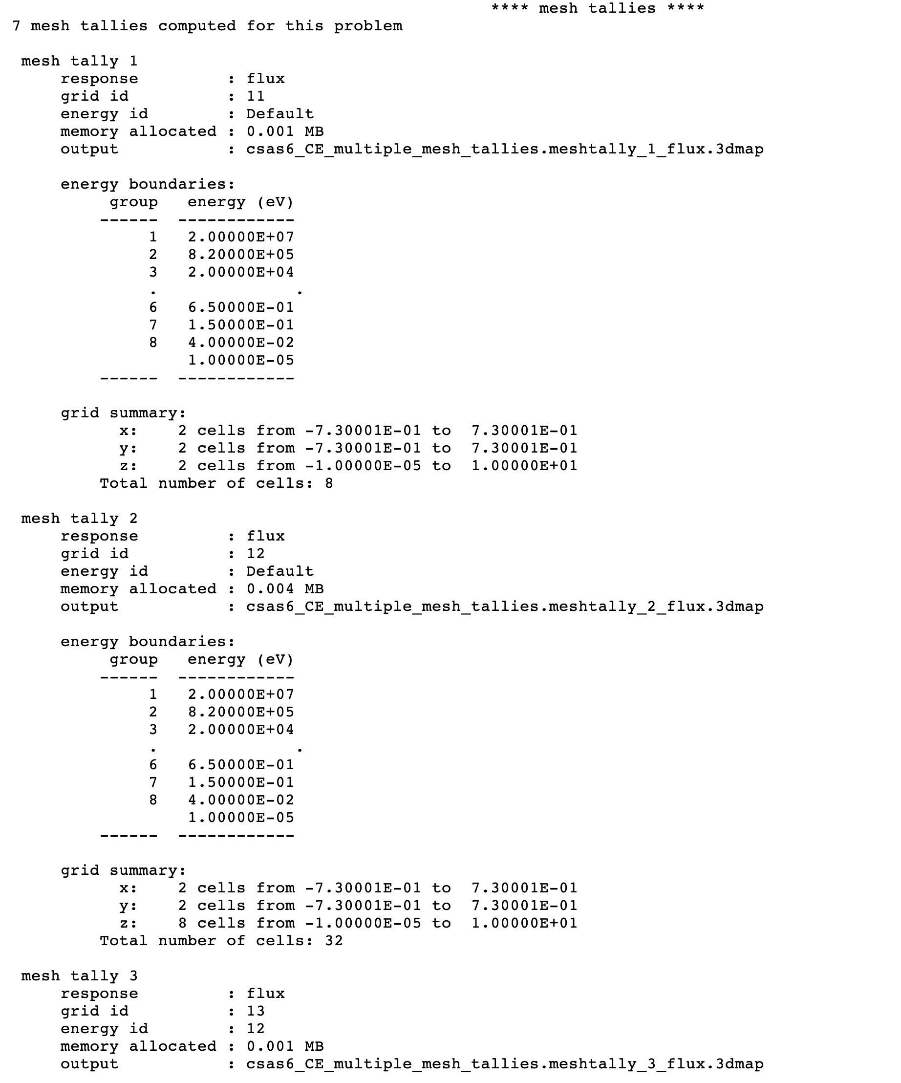
Fig. 2.1.6 Mesh tallies edit in KENO output
See the relevant subsections in Sect. 8.1.5 for further details for all these output edits.
2.1.4.2.3. Mesh tally output files
Depending on the user input specifications, the naming of the mesh tally 3dmap output files show some variations. Table 2.1.2 lists the 3dmap output filenames for each response type if only a single tally was requested for each response type. And, Table 2.1.3 lists the 3dmap output filenames for each response type if multiple mesh tallies are requested with the same response type. In such a case, the output filenames are updated with the keyword meshtally followed by the mesh id (mesh identifier used to define each mesh in tallies data).
response |
3dmap file name |
|
|
|
|
|
|
Note
Mesh tallies activated with old-style input method
(using the GFX, CDS, and FIS parameters) also
use the definitions for 3dmap file naming given
in Table 2.1.2.
response |
3dmap file name |
|
|
|
|
|
|
2.1.4.3. KENO data
Table 2.1.4 contains the outline for the KENO input. A typical KENO input is divided into 13 data blocks. A brief outline of commonly used data blocks is shown in Table 2.1.4. Note that parameter data must precede all other KENO data blocks when running standalone KENO codes; however, this is not applied to the KENO calculations performed as part of each CSAS sequence. As described in above sections, a minimal CSAS input always requires geometry data, and KENO data blocks listed in Table 2.1.4 can be defined in any order.
Information on all KENO input is provided in Sect. 8.1 of this document and will not be repeated here.
Type of data |
Starting flag |
Comments |
Termination flag |
|---|---|---|---|
Parameters |
READ PARAMETER |
Enter desired parameter data |
END PARAMETER |
Geometry |
READ GEOMETRY 1 |
Enter desired geometry data Always required by CSAS |
END GEOMETRY |
Array data |
READ ARRAY 1 |
Enter desired array data |
END ARRAY |
Boundary conditions |
READ BOUNDS |
Enter desired boundary conditions |
END BOUNDS |
Volume data |
READ VOLUME |
Enter desired volume data (KENO-VI only) |
END VOLUME |
Energy group boundaries |
READ ENERGY |
Enter desired neutron energy group boundaries |
END ENERGY |
Start data or initial source |
READ START |
Enter desired start data |
END START |
Plot data |
READ PLOT |
Enter desired plot data |
END PLOT |
Grid geometry data |
READ GRID |
Enter desired mesh data |
END GRID |
Reaction |
READ REACTION |
Enter desire reaction tallies (CE mode only) |
END REACTION |
KENO data terminus |
END DATA |
Enter to signal the end of all KENO. data |
|
1 Geometry input is different for both KENO V.a and KENO-VI See Sect. 8.1.3.4 for further details. |
|||
Note
Unlike standalone KENO calculations, each KENO data block can be entered in any order when running KENO codes as part of CSAS sequence.
2.1.5. Description of Output
This section contains a brief description and explanation of the CSAS sequence. As CSAS was designed as a SCALE control module/sequence its own output is minimal. To avoid duplicate output edits, it suppresses the output from KENO Data processor except a few diagnostic and warning messages while processing the KENO data blocks. Because the KENO Data processor and KENO codes produce the same output edits for some input data, capturing both output sections and keeping printing them may result in duplicate information in the output sections for those input data.
CSAS always captures the XSProc and KENO outputs and prints them in the code output. Because these output sections are described and their details are discussed in Sect. 8.1.5 and Sect. 7.1.1 and relevant XSProc sections, they will not be described in this section.
When CSAS is run with PARM=CHECK, only outputs from KENO Data processor and XSProc input processor are shown in the code output.
The sample output sections presented in this section were from one of the calculations performed by CSAS5. Here, only CSAS5 examples are given to prevent repetition because CSAS6 prints the same tables in the same format with the same content.
2.1.5.1. Program verification information
After the header page, program verification information is printed that lists the name of the program and the revision number. The job name, date, and time of execution are also printed as shown in Fig. 2.1.7. This information may be used for quality assurance purposes.
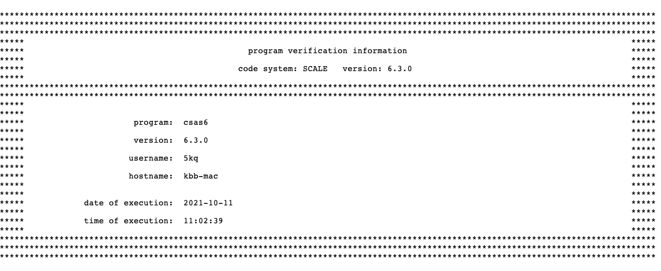
Fig. 2.1.7 Sample program verification table.
2.1.5.2. Mixture table
The first table printed by CSAS codes lists the compositions read and processed from the data entered in the composition data block. Basically, this table echos what user defined in the composition data block; data for each mixture are printed. First the mixture number, density, and temperature are printed, followed by a table of the nuclides which make up the mixture. This table contains the following data: mixture ID number, nuclide ZA number, atom density and temperature. A sample mixture table is shown in Fig. 2.1.8.
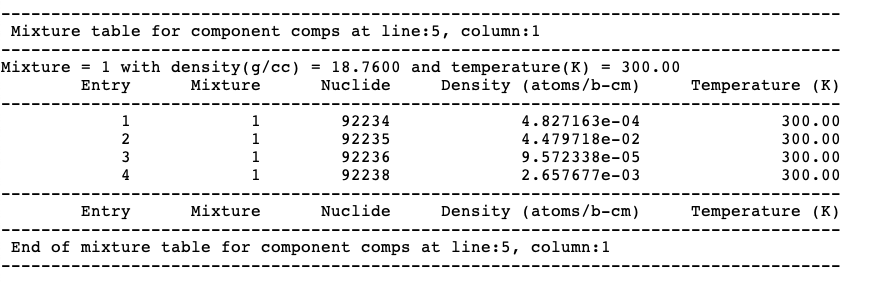
Fig. 2.1.8 An example of a mixture table.
Note
This output table prints only all mixtures read and
processed from the composition data block. Any mixture
defined with CELLMIX in celldata block is not printed here.
Note
The mixing table printed in KENO output may not
reflect the mixture properties listed in this output table.
Any mixture which is defined in composition data
block but not used in KENO transport process will not be
printed in KENO mixing table data edits. KENO also prints
the mixture data defined with CELLMIX or defined
in Double-het cell treatment in KENO mixing table data
edits in the output. See Sect. 8.1.3.10 for further
details about the KENO mixing data.
2.1.5.3. Cross section processing summary
In multigroup mode, cross section processing calculation path with XSProc show some differences depending on the type of the unit cells being processed and/or desired calculation methodology defined by user as discussed in Sect. 2.1.4.1. CSAS sequences summarize which of the XSProc calculation path is used when processing the unit cells in XSProc in the output.
A typical cross section processing summary table printed by a CSAS sequence in the code output is shown in Fig. 2.1.9.
The first record printed in this table is the multigroup cross section library which will be used in the calculations. This is followed by the cross section processing summary of the unit cells for this problem. This table includes the total number of unit cells being processed, and the number of unit cells processed with CENTRM and BONAMI calculations path. The last record printed in this table is the total elapsed time to process the XSProc data and build all the unit cells for the subsequent XSProc calculations.
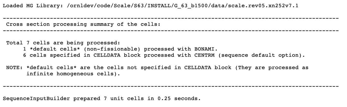
Fig. 2.1.9 Summary of cross section processing.
Caution
CSAS sequence always creates a unit cell for all the mixtures defined in the composition data block and stores them in a cell container. Then, XSProc cross section processing is applied to all the unit cells stored in the cell container regardless of whether they are used in KENO transport calculation. Performing cross section processing for the unused mixtures, especially fissile mixtures, might waste the allocated computational resources for this calculation.
2.1.6. Warning and error messages
CSAS sequence contains two types of warning and error messages. The first type of messages are from XSProc and SCALE sequence implementation which are common to many of the SCALE sequences. The second type of messages are mainly from the KENO Data processor as part of CSAS sequence implementation, and identified by CS- followed by a number. The details of the messages from KENO Data processor can be seen in Sect. 8.1.6.
Warning messages appear when a possible error is encountered. It is the responsibility of the user to verify whether the data are correct when a warning message is encountered. The functional modules, XSProc and KENO, activated by CSAS sequences will be executed if no error messages are generated and a warning message has been generated.
When an error is recognized, an error message is written and an error flag is set so the functional modules will not be activated. the code stops immediately if the error is too severe to allow continuation of input. However, it will continue to read and check the data if it is able. When the data reading is completed, execution is terminated if an error flag was set when the data were being processed. If the error flag has not been set, execution continues. When error messages are present in the output, the user should focus on the first error message, because subsequent messages may have been caused by the error that generated the first message.
The messages listed below complement the messages, which are from KENO Data processor, listed in KENO manual section, Sect. 8.1.6.
CS-21 A UNIT NUMBER WAS ENTERED FOR THE CROSS-SECTION LIBRARY. (LIB= IN PARAMETER DATA.) THE DEFAULT VALUE SHOULD BE USED IN ORDER TO UTILIZE THE CROSS SECTIONS GENERATED BY CSAS. MAKE CERTAIN THE CORRECT CROSS-SECTION LIBRARY IS BEING USED.
This message is from subroutine CPARAM. It indicates that a value has been entered for the cross-section library in the KENO V.a parameter data. The cross-section library created by the analytical sequence should be used. MAKE CERTAIN THAT THE CORRECT CROSS SECTIONS ARE BEING USED.
CS-55 *** ERRORS WERE ENCOUNTERED IN PROCESSING THE KENO DATA. EXECUTION IS IMPOSSIBLE. ***
This message from subroutine SASSY is printed if errors were found in the KENO input data for CSAS. When the data reading and checking have been completed, the problem will terminate without executing. Check the printout to locate the errors responsible for this message.
CS-62 *** ERROR *** MIXTURE ______ IN THE GEOMETRY WAS NOT CREATED IN THE STANDARD COMPOSITIONS SPECIFICATION DATA.
This message from subroutine MIXCHK indicates that a mixture specified in the KENO geometry was not created in the standard composition data.
CS-68 *** ERROR *** AN INPUT DATA ERROR HAS BEEN ENCOUNTERED IN THE ______ DATA ENTERED FOR THIS PROBLEM.
This message from the main program, CSAS, is printed if the subroutine library routine LRDERR returns a value of “TRUE,” indicating that a reading error has been encountered in the “KENO PARAMETER” data. The appropriate data type is printed in the message. Locate the unnumbered message stating “ERROR IN INPUT. CARD IMAGE PRINTED ON NEXT LINE”. Correct the data and resubmit the problem.
CS-69 ***ERROR*** MIXTURE ______ IS AN INAPPROPRIATE MIXTURE NUMBER FOR USE IN THE KENO GEOMETRY DATA BECAUSE IT IS A COMPONENT OF THE CELL-WEIGHTED MIXTURE CREATED BY XSDRNPM.
This message from subroutine CMXCHK indicates that a mixture that is a component of a cell-weighted mixture has been used in the KENO geometry data.
CS-100 *** ERROR *** THIS PROBLEM WILL NOT BE RUN BECAUSE ERRORS WERE ENCOUNTERED IN THE INPUT DATA.
This self-explanatory message indicates that an error occurred in input processing. User should examine the printout to locate the error or errors in the input data. Correct them and resubmit the problem.
2.1.7. Sample problems
This section contains example problems to demonstrate some of
capabilities available in CSAS with KENO codes.
A brief problem description and the associated input data for
multigroup mode of calculation are included for each problem.
The same sample problems may be executed in the continuous
energy mode by changing the library name from v7.1-252 to
ce_v7.1. The complete list of libraries distributed with
SCALE is provided in the Nuclear Data Libraries chapter.
2.1.7.1. CSAS5 sample problems
This section contains sample problems to demonstrate some of the options available in CSAS5. Note that sample problem 8 does not run in continuous-energy mode because they use CELLMIX or DOUBLEHET cell type.
2.1.7.1.1. CSAS5 sample problem 1: keff calculation
The purpose of this problem is to calculate the k-effective of a system. This problem is the same as the KENO V.a sample problem 12 in Appendix B except the cross-section library and KENO V.a mixing table are prepared by CSAS. The problem represents a critical experiment consisting of a composite array [CSAS5Tho64, CSAS5Tho73] of four highly-enriched (93.2%) uranium metal cylinders having a density of 18.76 g/cc and four 5.0677-L Plexiglas containers filled with uranyl nitrate solution. The uranium metal cylinders have a radius of 5.748 cm and a height of 10.765 cm. The uranyl nitrate solution has a specific gravity of 1.555 and contains 415 g of uranium per liter. The ID of the Plexiglas bottle is 19.05 cm and the inside height is 17.78 cm. The Plexiglas is 0.635 cm thick. The center-to-center spacing between the metal units is 13.18 cm in the Y direction and 13.45 cm in the Z direction. The center-to-center spacing between the solution units is 21.75 cm in the Y direction and 20.48 cm in the Z direction. The spacing between the Y-Z plane that passes through the centers of the metal units and the Y-Z plane that passes through the centers of the solution units is 17.465 cm in the X direction.
The metal units in this experiment are designated in Table II of [CSAS5Tho64] as cylinder index 11 and reflector index 1. A photograph of the experiment, Fig. 9 in [CSAS5Tho73], is given in Fig. 2.1.10.
=csas5   parm=(centrm)
sample problem set up 4aqueous 4 metal in csas5
v7.1-252
read composition
  uranium        1 0.985 300.  92235 93.2 92238 5.6 92234 1.0 92236 0.2 end
  solution
     mix=2
     rho[uo2(no3)2]= 415. 92235 92.6 92238 5.9 92234 1.0  92236 0.5
     molar[hno3]=9.783-3
     temperature=300
  end solution
  plexiglass     3 end
end composition
read param
  flx=yes fdn=yes nub=yes htm=no
end param
read geom
  unit 1
    com='uranyl nitrate solution in a plexiglas container'
    cylinder  2 1 9.525 2p8.89
    cylinder  3 1 10.16 2p9.525
    cuboid  0 1 4p10.875 2p10.24
  unit 2
    com='uranium metal cylinder'
    cylinder  1 1 5.748 2p5.3825
    cuboid  0 1 4p6.59 2p6.225
  unit 3
    com='1x2x2 array of solution units'
    array 1 3*0.0
  unit 4
    com='1x2x2 array of metal units padded to match solution array'
    array 2 3*0.0
    replicate 0 1 2*0.0 2*8.57 2*8.03 1
  global unit 5
    array 3 3*0.0
end geom
read array
  ara=1 nux=1 nuy=2 nuz=2 fill f1 end fill
  ara=2 nux=1 nuy=2 nuz=2 fill f2 end fill
  gbl=3 ara=3 nux=2 nuy=1 nuz=1
  com='composite array of solution and metal units'
  fill 4 3 end fill
end array
end data
end
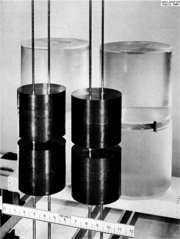
Fig. 2.1.10 Critical assembly of four solution units and four metal units.
2.1.7.1.2. CSAS5 Sample problem 8: k\(_{\infty}\) for a pebble bed fuel
This problem demonstrates setting up a fuel pebble from a pebble bed reactor, and calculating its \(k_{\boldsymbol{\infty}}\). The pebble consists of a fuel grain of UO2 0.025 cm in radius, coated with 0.003 cm of pyrolytic carbon, a further coat of 0.0035 cm thick silicon carbide, with a final coat of 0.004 cm thick pyrolytic carbon. 15000 grains are packed with graphite into an internal fuel sphere of 2.5 cm radius clad with a 0.5 cm thick covering of carbon and surrounded by helium. The fuel is 8.2% enriched 235U. The pebbles are stacked into an infinite square pitched array with a pitch of 6 cm.
This problem uses DOUBLEHET cell type, which is applicable only in the
multigroup mode of KENO calculations. Therefore, the continuous energy
version of this problem will end with an error message.
=csas5             parm=(centrm)
infinite array of pebbles on a square pitch
v7.1-252
read composition
' fuel kernel
  u-238  1 0 2.12877e-2 293.6 end
  u-235  1 0 1.92585e-3 293.6 end
  o      1 0 4.64272e-2 293.6 end
' inner pyro carbon
  c      3 0 9.52621e-2 293.6 end
' silicon carbide
  c      4 0 4.77240e-2 293.6 end
  si     4 0 4.77240e-2 293.6 end
' outer pyro carbon
  c      5 0 9.52621e-2 293.6 end
' graphite matrix
  c      6 0 8.77414e-2 293.6 end
' carbon pebble outer coating
  c      7 0 8.77414e-2 293.6 end
  he-3    8 0 3.71220e-11 293.6 end
  he-4    8 0 2.65156e-5 293.6 end
end composition
read celldata
  doublehet fuelmix=10 end
   gfr=0.025  1 coatt=0.004 3 coatt=0.0035 4 coatt=0.004 5
   matrix=6 numpar=15000 end grain
   centrm data
     ixprt=1 isn=8 nprt=2
   end centrm
  pebble sphsquarep right_bdy=white hpitch=3.0 8 fuelr=2.5 cladr=3.0 7 end
  centrm data
    ixprt=1 isn=8 nprt=2
  end centrm
end celldata
read param
  gen=210 npg=1000 htm=no
end param
read bounds
  all=mirror
end bounds
read geom
  global unit 1
    sphere   10 1 2.5
    sphere    7 1 3.0
    cuboid    8 1 6p3.0
end geom
end data
end
2.1.7.2. CSAS6 sample problems
This section contains sample problems to demonstrate some of the options available in CSAS6. A brief problem description and the associated input data for multigroup mode of calculation are included for each problem. The same sample problems may be executed in continuous-energy mode by changing the library name to an continuous-energy library. See Appendix A (Sect. 2.3) for additional examples.
2.1.7.2.1. CSAS6 Sample problem 1: Aluminum 30 Degree Pipe Angle Intersection
The purpose of this problem is to calculate the k-effective of a system composed of intersecting aluminum pipes, in the shape of a Y, filled with a 5% enriched UO2F2 solution. The UO2F2 solution at 299 K contains 907.0 gm/l of uranium, no excess acid, and has a specific gravity of 2.0289 gm/cm3. The assembly is composed of a 212.1 cm long vertical pipe and a second pipe that intersects the vertical pipe 76.7 cm from the outside bottom at an angle of 29.26 degrees with the upper vertical pipe. Both pipes have 13.95 cm inner diameters and 14.11 cm outer diameters. The vertical pipe is open on the top and 1.3 cm thick on the bottom. The Y-leg pipe, in the YZ-plane, is 126.04 cm in length with the sealed end 0.64 cm thick. The assembly is filled with solution to a height 129.5 cm above the outside bottom of the vertical pipe. From the point where the pipes intersect, the assembly is surrounded by water 37.0 cm in the \(\pm\)X directions, 100 cm in the +Y direction, -37 cm in the -Y direction, to the top of the assembly in the +Z direction, and -99.6 cm in the -Z direction.

Fig. 2.1.11 Critical assembly of UO2F2 solution in a 30\(^{\circ}\)-Y aluminum pipe.
=csas6
sample problem 1  Y-30, 5%uo2f2, 907.0g/l, 128.2, soln. ht.
v7.1-252
read comp
  solution
    mix=1
    rho[uo2f2]=907.0 92235 5.0 92238 95.0
    density=?
    temperature=299.0
  end solution
  al        2 1.0 end
  h2o       3 1.0 end
end comp
read parameters
  flx=yes fdn=yes far=yes pgm=yes plt=yes
end parameters
read start
  nst=6 tfx=0.0 tfy=0.0 tfz=0.0 lnu=1000
end start
read geometry
  global
  unit 1
    com='30 deg y'
    cylinder 10  13.95  135.4 -75.4
    cylinder 20  14.11  135.4 -76.7
    cylinder 30  13.95  125.4   0.0   rotate a2=-29.26
    cylinder 40  14.11  126.04  0.0   rotate a2=-29.26
    cuboid   50  2p37.0 100. -37.0 52.8 -75.4
    cuboid   60  2p37.0 100. -37.0 135.4 -99.6
    media  1  1 10  50
    media  2  1 20 -10 -30
    media  1  1 30  50 -10
    media  2  1 40 -30 -20
    media  0  1 10 -50
    media  0  1 30 -50 -10
    media  3  1 60 -20 -40 -10
    boundary  60
end geometry
read volume
    type=random  batches=1000
end volume
read plot
  scr=yes  lpi=10
  ttl='y-z slice at x=0.0  through centerline of both pipes'
  xul=0.0  yul=-39.0  zul=137.0
  xlr=0.0  ylr=105.0  zlr=-105.0
  vax=1    wdn=-1
  nax=400  end plt0
  ttl='x-y slice at z=26.0  slightly above point of separation'
  xul=-40.0 yul=105.0  zul=26.0
  xlr=+40.0 ylr=-40.0  zlr=26.0
  uax=1     vdn=-1
  nax=400 end plt1
  ttl='x-y slice at z=75.0  well above point of separation'
  xul=-40.0 yul=105.0  zul=75.0
  xlr=+40.0 ylr=-40.0  zlr=75.0
  uax=1     vdn=-1
  nax=400 end plt2
end plot
end data
end
2.1.7.2.2. CSAS6 Sample problem 2: Plexiglas Cross
The purpose of this problem is to calculate the k-effective of a system composed of intersecting Plexiglas pipes, in the shape of a cross, filled with a 5% enriched UO2F2 solution. The room temperature UO2F2 solution contains 896.1 gm/l of uranium, no excess acid, and has a specific gravity of 2.015 gm/cm3. The pipes have a 13.335 cm inner diameter and 16.19 cm outer diameter. The vertical pipe is open on the top and 3.17 cm thick on the bottom. The horizontal pipe ends are 3.17 thick. The vertical pipe is 210.19 cm in length and filled with solution to a height of 117.2 cm. The two horizontal legs, positioned in the XZ-plane, intersect the vertical pipe 91.44 cm from the outside bottom at an 89 degree angle with the upper section of the pipe. Each horizontal is 91.44 cm in length and filled with the above specified UO2F2 solution. A water reflector surrounding the solution filled pipes extends out from the point where the pipes intersect 111.76 cm in the \(\pm\)X directions, 20.64 cm in the \(\pm\)Y directions, 29.03 cm in the +Z direction, and -118.428 cm in the -Z direction.
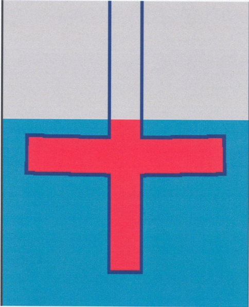
Fig. 2.1.12 Critical assembly of UO2F2 solution in a Plexiglas cross.
=csas6
sample problem 2  89-cross, 5% uo2f2 soln, plexiglass pipes, h2o refl.
v7.1-252
read comp
  solution
    mix=1
    rho[uo2f2]=896.1 92235 5.0 92238 95.0
    density=?
    temperature=298.0
  end solution
  plexiglass 3 1.0 end
  h2o        2 1.0 end
end comp
read param
  plt=yes
end param
read geom
  global unit 1
    cylinder  10  13.335 28.93 -88.27
    cylinder  20  13.335 121.92 -88.27
    cylinder  30  16.19 121.92 -91.44
    cylinder  40  13.335 88.27 0.0 rotate a1=90. a2=89.
    cylinder  50  16.19  91.44 0.0 rotate a1=90. a2=89.
    cylinder  60  13.335 88.27 0.0 rotate a1=-90. a2=89.
    cylinder  70  16.19  91.44 0.0 rotate a1=-90. a2=89.
    cuboid    80  2p111.74 2p20.64 29.03 -118.428
    cuboid    90  2p111.74 2p40.64 121.92 -118.428
    media 1 1 10
    media 0 1 20 -10
    media 3 1 30 -10 -20 -50 -70
    media 1 1 40 -10 -20
    media 3 1 50 -40 -10 -20
    media 1 1 60 -10 -20
    media 3 1 70 -60 -10 -20 -50
    media 2 1 80 -10 -20 -30 -40 -50 -60 -70
    media 0 1 90 -20 -30 -80
    boundary  90
end geom
read volume
   type=trace
end volume
read start
  nst=6  tfx=0. tfy=0. tfz=0. lnu=1000
end start
read plot
  scr=yes  lpi=10
  ttl=' x-z slice at y=0.0 '
  xul=-113. yul=0. zul=  48.
  xlr= 113. ylr=0. zlr=-120.
  uax=1.0   wdn=-1.0
  nax=400  end plt0
  ttl=' y-z slce at x=0.0 '
  xul=0.    yul=-42. zul= 122.
  xlr=0.    ylr= 42. zlr=-120.
  vax=1.0   wdn=-1.0
  nax=400  end plt1
  ttl=' x-y slice at z=0.0 '
  xul=-113.0 yul= 42. zul=0.
  xlr= 113.0 ylr=-42. zlr=0.
  uax=1.0    vdn=-1.0
  nax=400  end plt2
end plot
end data
end
2.1.7.2.3. CSAS6 Sample problem 3: Sphere
This problem models an assembly consisting of a 93.2% enriched bare uranium sphere, 8.741 cm in radius, having a density of 18.76 gm/cm3. Problem 3 models the assembly as a single bare sphere. The second problem models the assembly as a hemisphere with mirror reflection on the flat surface. The next three problems model the sphere using chords. This set of four problems is designed to illustrate the use of multiple chords in a problem.
=csas6
sample problem 3  bare 93.2% enriched uranium sphere
v7.1-252
read comp
  uranium  1 den=18.76 1 293 92235 93.2 92238 5.6 92234 1.0 92236 0.2 end
end comp
read geometry
  global unit 1
    sphere 10  8.741
    cuboid   20  6p8.741
    media  1 1 10      vol=2797.5121
    media  0 1 20 -10  vol=2545.3424
    boundary 20
end geometry
end data
end
2.1.7.2.4. CSAS6 Sample problem 4: Sphere Models Using Chords and Mirror Albedos
This problem models an assembly consisting of a 93.2% enriched bare uranium sphere, 8.741 cm in radius, having a density of 18.76 gm/cm3. The problem models the assembly as a hemisphere with mirror reflection on the flat surface.
=csas6
sample problem 4  bare 93.2% U sphere, hemisphere w/ mirror albedo
v7.1-252
read comp
  uranium  1 den=18.76 1 293 92235 93.2 92238 5.6 92234 1.0 92236 0.2 end
end comp
read geometry
  global unit 1
    sphere 10  8.741  chord +x=0.0
    cuboid   20  8.741 0.0  8.741 -8.741 8.741 -8.741
    media  1 1 10      vol=2797.5121
    media  0 1 20 -10  vol=2545.3424
    boundary 20
end geometry
read bounds
  -xb=mirror
end bounds
end data
end
2.1.7.2.5. CSAS6 Sample problem 5: Sphere Models Using Chords and Mirror Albedos
This problem models an assembly consisting of a 93.2% enriched bare uranium sphere, 8.741 cm in radius, having a density of 18.76 gm/cm3. The problem models the assembly as a quarter sphere with mirror reflection on the two flat surfaces.
=csas6
sample problem 5  bare 93.2% U sphere, quarter sphere w/ mirror albedo
v7.1-252
read comp
  uranium  1 den=18.76 1 293 92235 93.2 92238 5.6 92234 1.0 92236 0.2 end
end comp
read geometry
  global unit 1
    sphere 10  8.741  chord +x=0.0  chord  +y=0.0
    cuboid   20  8.741 0.0 8.741 0.0 8.741 -8.741
    media  1 1 10      vol=2797.5121
    media  0 1 20 -10  vol=2545.3424
    boundary 20
end geometry
read bounds
  -xy=mirror
end bounds
end data
end
2.1.7.2.6. CSAS6 Sample problem 6: Sphere Models Using Chords and Mirror Albedos (Eighth Sphere)
This problem models an assembly consisting of a 93.2% enriched bare uranium sphere, 8.741 cm in radius, having a density of 18.76 gm/cm3. The problem models the assembly as an eighth sphere with mirror reflection on the three flat surfaces.
=csas6
sample problem 6  bare 93.2% U sphere, eighth sphere w/ mirror albedo
v7.1-252
read comp
  uranium  1 den=18.76 1 293 92235 93.2 92238 5.6 92234 1.0 92236 0.2 end
end comp
read geometry
  global unit 1
    sphere 10  8.741  chord +x=0.0  chord  +y=0.0  chord +z=0.0
    cuboid   20  8.741 0.0 8.741 0.0 8.741 0.0
    media  1 1 10      vol=2797.5121
    media  0 1 20 -10  vol=2545.3424
    boundary 20
end geometry
read bounds
  -fc=mirror
end bounds
end data
end
2.1.7.2.7. CSAS6 Sample problem 7: Grotesque without the Diaphragm
The purpose of this problem is to calculate the keff of a system composed of eight enriched uranium units placed on a diaphragm, with an irregularly shaped centerpiece positioned in the center hole of the diaphragm [CSAS5Mih99]. The assembly and centerpiece are shown in Fig. 2.1.13, which is Fig. 4 from [CSAS5Mih99]. The eight units consist of an approximate parallelepiped with an irregular top, a parallelepiped, and six cylinders of various sizes. The centerpiece, which penetrates the hole in the diaphragm, consists of a cylinder topped by a parallelepiped topped by a hemisphere. The diaphragm is not modeled in this example.
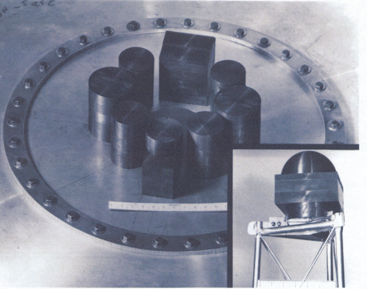
Fig. 2.1.13 Grotesque experimental setup.
=csas6
sample problem 7  keno-vi grotesque w/o diaphragm, ornl/csd/tm-220
v7.1-252
read comp
  uranium   1 den=18.76 1 293 92235 93.2 92238 5.6 92234 1.0 92236 0.2 end
  uranium   2 den=18.76 1 293 92235 93.2 92238 5.6 92234 1.0 92236 0.2 end
  uranium   3 den=18.76 1 293 92235 93.2 92238 5.6 92234 1.0 92236 0.2 end
  uranium   4 den=18.76 1 293 92235 93.2 92238 5.6 92234 1.0 92236 0.2 end
  uranium   5 den=18.76 1 293 92235 93.2 92238 5.6 92234 1.0 92236 0.2 end
  uranium   6 den=18.76 1 293 92235 93.2 92238 5.6 92234 1.0 92236 0.2 end
  uranium   7 den=18.76 1 293 92235 93.2 92238 5.6 92234 1.0 92236 0.2 end
  uranium   8 den=18.76 1 293 92235 93.2 92238 5.6 92234 1.0 92236 0.2 end
  uranium   9 den=18.76 1 293 92235 93.2 92238 5.6 92234 1.0 92236 0.2 end
  uranium  10 den=18.76 1 293 92235 93.2 92238 5.6 92234 1.0 92236 0.2 end
  uranium  11 den=18.76 1 293 92235 93.2 92238 5.6 92234 1.0 92236 0.2 end
  uranium  12 den=18.76 1 293 92235 93.2 92238 5.6 92234 1.0 92236 0.2 end
  uranium  13 den=18.76 1 293 92235 93.2 92238 5.6 92234 1.0 92236 0.2 end
  uranium  14 den=18.76 1 293 92235 93.2 92238 5.6 92234 1.0 92236 0.2 end
end comp
read param
  pgm=yes plt=yes
end param
read geom
  global unit 1
'*** one through three is item 1 in drawing 84-10649 ornl/csd/tm-220 ***
'one    top piece of item 1
  cuboid 10  2p6.3515 1.2685 -3.8115 13.377 13.058 origin y=-17.464 z=0.15 rotate a2=-1.35
'two    middle piece of item 1
  cuboid 20  2p6.3515 6.3515 -3.8115 13.058 11.155 origin y=-17.464 z=0.15 rotate a2=-1.35
'three  bottom piece of item 1
  cuboid 30  4p6.3515 11.155 0. origin y=-17.464 z=0.15 rotate a2=-1.35
'*** four is item 2 in drawing 84-10649 ornl/csd/tm-220 ***
  cylinder 40 4.555 12.918 0.        origin x=-12.176 y=-9.343 z=0.111 rotate a1=-52.5 a2=-1.400
'*** five is item 3 in drawing 84-10649 ornl/csd/tm-220 ***
  cylinder 50 5.761 13.475 0.        origin x=-16.333 y=1.681 z=0.174 rotate a1=83.5 a2=+1.173
'*** six is item 4 in drawing 84-10649 ornl/csd/tm-220 ***
  cylinder 60 4.5525 12.969 0.    origin x=-9.539 y=11.168 z=0.156 rotate a1=40.5 a2=+1.970
'*** seven and eight are item 5 in drawing 84-10649 ornl/csd/tm-220 ***
'seven
  cuboid  70  2p3.81 8.13 -4.573 8.91 0. origin y=15.698 z=0.290 rotate a2=+2.58
'eight
  cylinder 80 4.573 13.229 8.91   origin y=15.698 z=0.290 rotate a2=+2.58
'*** nine is item 6 in drawing 84-10649 ornl/csd/tm-220 ***
  cylinder 90 4.5545 12.974 0.    origin x=9.854 y=10.964 z=0.134 rotate a1=-42.0 a2=+1.680
'*** ten is item 7 in drawing 84-10649 ornl/csd/tm-220 ***
  cylinder 100 5.7495 13.475 0.    origin x=16.388 y=1.434 z=0.140 rotate a1=-86.0 a2=+1.400
'*** eleven is item 8 in drawing 84-10649 ornl/csd/tm-220 ***
  cylinder 110 4.5565 12.954 0.    origin x=12.029 y=-9.398 z=0.087 rotate a1=38.0 a2=-1.100
'*12 through 14 is the centerpiece in drawing 84-10649 ornl/csd/tm-220
'twelve
  cylinder 120 5.757 2.690 0.      origin x=-0.593 y=-0.593 z=-1.753
'thirteen
  cuboid 130 4p6.35 5.718 0.       origin z=0.937
'fourteen
  sphere    140 6.082 chord +z=0.   origin x=-0.268 y=0.268 z=6.655
'*** fifteen is the system boundary ***
'fifteen
  cuboid   150 4p25.0 15.0 -2.0
  media  1 1 +10       vol=20.58546556
  media  2 1 +20 -10   vol=245.678420867
  media  3 1 +30 -20   vol=1800.040061395
  media  4 1 +40       vol=842.019046637
  media  5 1 +50       vol=1404.99376489
  media  6 1 +60       vol=844.415646269
  media  7 1 +70       vol=862.4600226
  media  8 1 +80 -70   vol=283.749744681
  media  9 1 +90       vol=845.483582679
  media 10 1 +100      vol=1399.390119093
  media 11 1 +110      vol=844.921798001
  media 12 1 +120 -130 vol=280.088070346
  media 13 1 +130      vol=922.25622
  media 14 1 +140 -130 vol=471.191948666
  media 0 1 150 -10 -20 -30 -40 -50 -60 -70 -80 -90 -100
            -110 -120 -130 -140  vol=31432.726088316
  boundary 150
end geom
read plot
  scr=yes  lpi=10
           clr= 1 255   0   0
                2   0   0 205
                3   0 229 238
                4   0 238   0
                5 205 205   0
                6 255 121 121
                7 145  44 238
                8 150 150 150
                9 240 200 220
               10   0 191 255
               11 224 255 255
               12   0 128  64
               13 255 202 149
               14 255   0 128
            end color
  ttl='grotesque x-y slice at z=0.5'
  xul=-25.5 yul= 25.5 zul=0.5
  xlr= 25.5 ylr=-25.5 zlr=.5
  uax=1     vdn=-1  nax=800 end
  ttl='grotesque x-y slice at z=2.0'
  xul=-25.5 yul= 25.5 zul=2
  xlr= 25.5 ylr=-25.5 zlr=2 end
  ttl='grotesque x-y slice at z=9.5'
  xul=-25.5 yul= 25.5 zul=9.5
  xlr= 25.5 ylr=-25.5 zlr=9.5 end
  ttl='grotesque y-z slice at x=-0.593'
  xul=-.593 yul=-25.5 zul=15.5
  xlr=-.593 ylr= 25.5 zlr=-3.5
  uax=0     vax=1
  vdn=0     wdn=-1 nax=800  end
  ttl='grotesque x-z slice at y=0.0'
  xul=-25.5 yul=0.0  zul=15.5
  xlr= 25.5 ylr=0.0  zlr=-3.5
  uax=1     vax=0    wax=0
  udn=0     vdn=0    wdn=-1 nax=800  end
  ttl='grotesque x-z slice at y=12.125'
  xul=-25.5 yul=12.125  zul=15.5
  xlr= 25.5 ylr=12.125  zlr=-3.5
  uax=1     vax=0       wax=0
  udn=0     vdn=0       wdn=-1 nax=800  end
  ttl='grotesque x-z slice at y=-12.000'
  xul=-25.5 yul=-12.000  zul=15.5
  xlr= 25.5 ylr=-12.000  zlr=-3.5
  uax=1     vax=0        wax=0
  udn=0     vdn=0        wdn=-1 nax=800  end
end plot
end data
end
2.1.7.2.8. CSAS6 Sample problem 8 Infinite Array of MOX and UO2 Assemblies
The purpose of this problem is to calculate the keff of a system composed of an infinite array of MOX assemblies interspersed between UO2 assemblies. Both assembly types contain 331 pins in a hexagonal lattice with a pin pitch of 1.275 cm and an assembly pitch of 23.60 cm as shown in Fig. 2.1.14. The moderator is borated water at 306\(^{\circ}\)C having a density of 0.71533 gm/cc and composed of 99.94 wt % H2O and 0.06 wt % natural boron. Each fuel rod is 355 cm in length, has a radius of 0.3860 cm, 0.722-cm-thick Zr cladding with no gap, and is at a temperature of 754\(^{\circ}\)C.
The UO2 fuel consists of 4.4 wt % 235U and 95.6 wt % 238U at a density of 8.7922 gm/cc. The UO2 fuel also contains 9.4581E-9 atoms/b-cm of 135Xe and 7.3667E-8 atoms/b-cm of 149Sm.
The MOX fuel consists of 96.38 wt % UO2 and 3.62 wt % PuO2 at a density of 8.8182 gm/cc. The UO2 fuel is composed of 2.0 wt % 235U and 98.0 wt % 238U. The PuO2 fuel is composed of 93.0 wt % 239Pu, 6.0 wt % 240Pu- and 1.0 wt % 241Pu. The MOX fuel also contains 9.4581E-9 atoms/b-cm of 135Xe and 7.3667E-8 atoms/b-cm of 149Sm.
These two assemblies are placed so they represent an infinite array in the X and Y dimensions as shown in Fig. 2.1.15. There is 20 cm of water above and below fuel assemblies. This problem uses CENTRM/PMC as the resolved resonance processor cross section. Since an infinite array cannot be explicitly modeled, a section of the array is modeled and the X and Y sides have mirror reflection.
=csas6        parm=(centrm)
sample problem 8 - VVER inf. array - MOX & UO2 Assemblies
v7.1-252
read comp
'  UO2 Fuel
    uo2     1 den=8.7922 1.0 1027 92235 4.4  92238 95.6 end
    xe-135  1 0 9.4581E-09 1027 end
    sm-149  1 0 7.3667E-08 1027 end
'  MOX Fuel
    uo2     2 den=8.8182 0.9638 1027  92235  2.0 92238 98.0 end
    puo2    2 den=8.8182 0.0362 1027  94239 93.0 94240  6.0 94241  1.0 end
    xe-135  2 0 9.4581E-09 1027 end
    sm-149  2 0 7.3667E-08 1027 end
'  Cladding for UO2 fuel
    zr      3 den=6.4073 1.0  579  end
'  Moderator for UO2 fuel
    h2o     4 den=0.71533 0.9994 579 end
    boron   4 den=0.71533 0.0006 579 end
'  Cladding for MOX fuel
    zr      5 den=6.4073 1.0  579  end
'  Moderator for MOX fuel
    h2o     6 den=0.71533 0.9994 579 end
    boron   6 den=0.71533 0.0006 579 end
'  Moderator for vacant units
    h2o     7 den=0.71533 0.9994 579 end
    boron   7 den=0.71533 0.0006 579 end
end comp
read celldata
  latticecell triangpitch pitch=1.2750 4 fueld=0.7720 1 cladd=0.9164 3 end
  latticecell triangpitch pitch=1.2750 6 fueld=0.7720 2 cladd=0.9164 5 end
'  more data  dab=500  end more
end celldata
read param
  gen=203  npg=1000
end param
read bounds
  all=mirror zfc=void
end bounds
read geom
  unit   1
   com='UO2 Fuel Rod'
   cylinder 10 0.3860 355.0 0.0
   cylinder 20 0.4582 355.0 0.0
   hexprism 30 0.6375 355.0 0.0
   media 1 1 10
   media 3 1 20 -10
   media 4 1 30 -20
   boundary 30
  unit  2
   com='Vacant(water filled) hex'
   hexprism 10 0.6375 355.0 0.0
   media 7 1 10
   boundary 10
  unit  3
   com='Vacant(water filled) hex'
   hexprism 10 0.6375 355.0 0.0
   media 7 1 10
   boundary 10
  unit   4
   com='MOX Fuel Rod'
   cylinder 10 0.3860 355.0 0.0
   cylinder 20 0.4582 355.0 0.0
   hexprism 30 0.6375 355.0 0.0
   media 2 1 10
   media 5 1 20 -10
   media 6 1 30 -20
   boundary 30
  global unit 5
   rhexprism 10 11.800 355.0 0.0
   rhexprism 20 11.800 355.0 0.0 origin y=23.6
   rhexprism 30 11.800 355.0 0.0 origin x=20.4382 y=11.8
   rhexprism 40 11.800 355.0 0.0 origin x=20.4382 y=35.4
   cuboid   50 20.4382 0.0 35.4 0.0 375.0 -20.0
   array 1  10 -20 -30 -40 place 12 12 1  0.0       0.0  0.0
   array 2  20 -10 -30 -40 place 12 12 1  0.0      23.6  0.0
   array 2  30 -10 -20 -40 place 12 12 1  20.4382  11.8  0.0
   array 1  40 -10 -20 -30 place 12 12 1  20.4382  35.4  0.0
   media 4 1 50 -10 -20 -30 -40
   boundary 50
end geom
read array
  ara=1 typ=shexagonal nux=23 nuy=23 nuz=1
    fill
   3 3 3 3 3 3 3 3 3 3 3 3 3 3 3 3 3 3 3 3 3 3 3
    3 3 3 3 3 3 4 4 4 4 4 4 4 4 4 4 4 3 3 3 3 3 3
   3 3 3 3 3 3 4 4 4 4 4 4 4 4 4 4 4 4 3 3 3 3 3
    3 3 3 3 3 4 4 4 4 4 4 4 4 4 4 4 4 4 3 3 3 3 3
   3 3 3 3 3 4 4 4 4 4 4 4 4 4 4 4 4 4 4 3 3 3 3
    3 3 3 3 4 4 4 4 4 4 4 4 4 4 4 4 4 4 4 3 3 3 3
   3 3 3 3 4 4 4 4 4 4 4 4 4 4 4 4 4 4 4 4 3 3 3
    3 3 3 4 4 4 4 4 4 4 4 4 4 4 4 4 4 4 4 4 3 3 3
   3 3 3 4 4 4 4 4 4 4 4 4 4 4 4 4 4 4 4 4 4 3 3
    3 3 4 4 4 4 4 4 4 4 4 4 4 4 4 4 4 4 4 4 4 3 3
   3 3 4 4 4 4 4 4 4 4 4 4 4 4 4 4 4 4 4 4 4 4 3
    3 4 4 4 4 4 4 4 4 4 4 4 4 4 4 4 4 4 4 4 4 4 3
   3 3 4 4 4 4 4 4 4 4 4 4 4 4 4 4 4 4 4 4 4 4 3
    3 3 4 4 4 4 4 4 4 4 4 4 4 4 4 4 4 4 4 4 4 3 3
   3 3 3 4 4 4 4 4 4 4 4 4 4 4 4 4 4 4 4 4 4 3 3
    3 3 3 4 4 4 4 4 4 4 4 4 4 4 4 4 4 4 4 4 3 3 3
   3 3 3 3 4 4 4 4 4 4 4 4 4 4 4 4 4 4 4 4 3 3 3
    3 3 3 3 4 4 4 4 4 4 4 4 4 4 4 4 4 4 4 3 3 3 3
   3 3 3 3 3 4 4 4 4 4 4 4 4 4 4 4 4 4 4 3 3 3 3
    3 3 3 3 3 4 4 4 4 4 4 4 4 4 4 4 4 4 3 3 3 3 3
   3 3 3 3 3 3 4 4 4 4 4 4 4 4 4 4 4 4 3 3 3 3 3
    3 3 3 3 3 3 4 4 4 4 4 4 4 4 4 4 4 3 3 3 3 3 3
   3 3 3 3 3 3 3 3 3 3 3 3 3 3 3 3 3 3 3 3 3 3 3
    end fill
  ara=2 typ=shexagonal nux=23 nuy=23 nuz=1
    fill
   2 2 2 2 2 2 2 2 2 2 2 2 2 2 2 2 2 2 2 2 2 2 2
    2 2 2 2 2 2 1 1 1 1 1 1 1 1 1 1 1 2 2 2 2 2 2
   2 2 2 2 2 2 1 1 1 1 1 1 1 1 1 1 1 1 2 2 2 2 2
    2 2 2 2 2 1 1 1 1 1 1 1 1 1 1 1 1 1 2 2 2 2 2
   2 2 2 2 2 1 1 1 1 1 1 1 1 1 1 1 1 1 1 2 2 2 2
    2 2 2 2 1 1 1 1 1 1 1 1 1 1 1 1 1 1 1 2 2 2 2
   2 2 2 2 1 1 1 1 1 1 1 1 1 1 1 1 1 1 1 1 2 2 2
    2 2 2 1 1 1 1 1 1 1 1 1 1 1 1 1 1 1 1 1 2 2 2
   2 2 2 1 1 1 1 1 1 1 1 1 1 1 1 1 1 1 1 1 1 2 2
    2 2 1 1 1 1 1 1 1 1 1 1 1 1 1 1 1 1 1 1 1 2 2
   2 2 1 1 1 1 1 1 1 1 1 1 1 1 1 1 1 1 1 1 1 1 2
    2 1 1 1 1 1 1 1 1 1 1 1 1 1 1 1 1 1 1 1 1 1 2
   2 2 1 1 1 1 1 1 1 1 1 1 1 1 1 1 1 1 1 1 1 1 2
    2 2 1 1 1 1 1 1 1 1 1 1 1 1 1 1 1 1 1 1 1 2 2
   2 2 2 1 1 1 1 1 1 1 1 1 1 1 1 1 1 1 1 1 1 2 2
    2 2 2 1 1 1 1 1 1 1 1 1 1 1 1 1 1 1 1 1 2 2 2
   2 2 2 2 1 1 1 1 1 1 1 1 1 1 1 1 1 1 1 1 2 2 2
    2 2 2 2 1 1 1 1 1 1 1 1 1 1 1 1 1 1 1 2 2 2 2
   2 2 2 2 2 1 1 1 1 1 1 1 1 1 1 1 1 1 1 2 2 2 2
    2 2 2 2 2 1 1 1 1 1 1 1 1 1 1 1 1 1 2 2 2 2 2
   2 2 2 2 2 2 1 1 1 1 1 1 1 1 1 1 1 1 2 2 2 2 2
    2 2 2 2 2 2 1 1 1 1 1 1 1 1 1 1 1 2 2 2 2 2 2
   2 2 2 2 2 2 2 2 2 2 2 2 2 2 2 2 2 2 2 2 2 2 2
    end fill
end array
read plot
  lpi=10 scr=yes
  ttl='VVER assembly x-y x-section'
  xul=-0.1  yul=35.5  zul=10
  xlr=20.6  ylr=-0.1  zlr=10
  uax=1     vdn=-1.0
  nax=640   pic=mat   end plt1
end plot
read volume
    type=random  batches=1000
end volume
end data
end
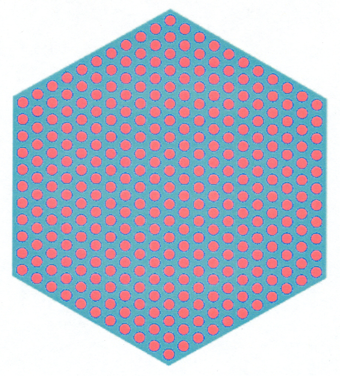
Fig. 2.1.14 MOX or UO2 hexagonal assembly.
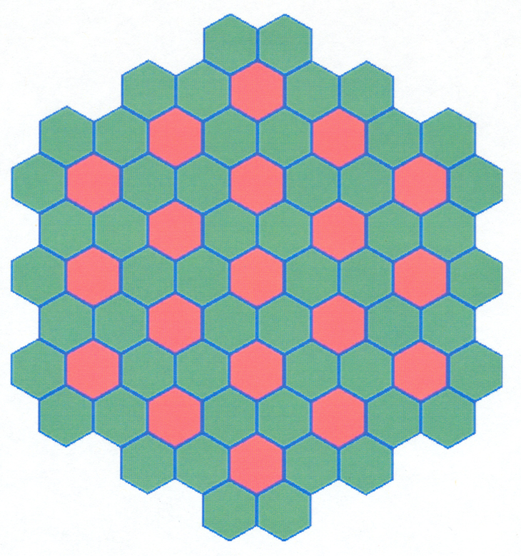
Fig. 2.1.15 Infinite array of MOX assemblies interspersed between UO2 assemblies.
References
- CSAS5Mih99(1,2)
J. T. Mihalczo. Brief summary of unreflected and unmoderated cylindrical critical experiments with oralloy at Oak Ridge. Technical Report, Oak Ridge National Laboratory, Oak Ridge, TN (USA), 1999.
- CSAS5Tho64(1,2)
J. T. Thomas. CRITICAL THREE-DIMENSIONAL ARRAYS OF NEUTRON-INTERACTING UNITS. PART II. U (93.2) METAL. Technical Report, Oak Ridge National Laboratory, Oak Ridge, TN (USA), 1964.
- CSAS5Tho73(1,2)
Joseph T. Thomas. Critical three-dimensional arrays of U (93.2)-metal cylinders. Nuclear Science and Engineering, 52(3):350–359, 1973. Publisher: Taylor & Francis.