8.1. KENO: A Monte Carlo Criticality Program

K. B. Bekar, C. Celik, M. E. Dunn,¹ S. Goluoglu,¹ D. F. Hollenbach,¹ N. F. Landers,¹ C. M.Perfetti,¹ L. M. Petrie,¹ B. T. Rearden,¹

KENO is a three-dimensional (3D) Monte Carlo criticality transport program developed and maintained for use as part of the SCALE Code System. It can be used as part of a sequence or as a standalone program. There are two versions of the code currently supported in SCALE. KENO V.a is the older of the two. KENO-VI contains all current KENO V.a features plus a more flexible geometry package known as the SCALE Generalized Geometry Package. The geometry package in KENO-VI is capable of modeling any volume that can be constructed using quadratic equations. In addition, such features as geometry intersections, body rotations, hexagonal and dodecahedral arrays, and array boundaries have been included to make the code more flexible.

The simpler geometry features supported by KENO V.a allow for significantly shorter execution times than KENO-VI, while the additional geometry features supported in KENO-VI make the code appropriate for cases where geometry modeling is not possible with KENO V.a. In particular, KENO-VI allows intersections, body truncations with planes, and a much wider variety of geometrical bodies. KENO-VI also has the ability to rotate bodies so that volumes no longer must be positioned parallel to a major axis. Hexagonal arrays are available in KENO-VI and dohecahedral arrays enable the code to model pebble bed reactors and other systems composed of close packed spheres. The use of array boundaries makes it possible to fill a non-cuboidal volume with an array, specifying the boundary where a particle leaves and enters the array.

Except for geometry capabilities, the two versions of KENO share most of the computational capabilities and the input flexibility specific to most SCALE modules. They can both operate in multigroup or continuous energy mode, run as standalone codes, or integrated in computational sequences such as CSAS, TSUNAMI-3D, or TRITON. Both versions of the code are continually updated and are written in FORTRAN 90.

Computational capabilities shared by the two versions of KENO include the determination of k-effective, neutron lifetime, generation time, energy-dependent leakages, energy- and region-dependent absorptions, fissions, the system mean-free-path, the region-dependent mean-free-path, average neutron energy, flux densities, fission densities, reaction rate tallies, mesh tallies, source convergence diagnostics, problem-dependent continuous energy temperature treatments, parallel calculations, restart capabilities, and many more.

¹Formerly with Oak Ridge National Laboratory

8.1.1. ACKNOWLEDGMENTS

Many individuals have contributed significantly to the development of KENO. Special recognition is given to G. E. Whitesides, former Director of the Computing Applications Division, who was responsible for the concept and development of the original KENO code. He has also contributed significantly to some of the techniques used in both KENO versions. The late J. T. Thomas offered many ideas that have been implemented in the code. R. M. Westfall, retired from ORNL, provided early consultation, encouragement, and benchmarks for validating the code. The special abilities of J. R. Knight, retired from ORNL, contributed substantially to debugging early versions of the code. S. W. D. Hart was instrumental in implementing continuous energy temperature treatments. W. J. Marshall has provided substantial validation and quality assurance reviews. Appreciation is expressed to C. V. Parks and S. M. Bowman for their support of KENO and the KENO3D visualization tool. The late P. B. Fox provided many of the figures in this document. D. Ilas, B. J. Marshall, and D. E. Mueller consolidated the previous KENO V.a and KENO-VI manuals into this present form. The efforts of L. F. Norris (retired), W. C. Carter (retired), S. J. Poarch, D. J. Weaver (retired), S. Y. Walker and R. B. Raney in preparing this document are gratefully acknowledged.

The authors thank the U. S. Nuclear Regulatory Commission and the DOE Nuclear Criticality Safety Program for sponsorship of the continuous energy, source convergence diagnostics, and grid geometry features in the current version.

8.1.2. Introduction to KENO

KENO, a functional module in the SCALE system, is a Monte Carlo criticality program used to calculate \(k_{eff}\), fluxes, reaction rates, and other data for three-dimensional (3-D) systems. Special features include multigroup or continuous energy mode, simplified data input, the ability to specify origins for spherical and cylindrical geometry regions, a P_n scattering treatment, and restart capability.

The KENO data input features flexibility in the order of input. The only restrictions are that the sequence identifier, title, and cross section library must be entered first. A large portion of the data has been assigned default values found to be adequate for many problems. This feature enables the user to run a problem with a minimum of input data.

In addition to the features listed above, KENO-VI uses the SCALE Generalized Geometry Package (SGGP), which contains a much larger set of geometrical bodies, including cuboids, cylinders, spheres, cones, dodecahedrons, elliptical cylinders, ellipsoids, hoppers, parallelepipeds, planes, rhomboids, and wedges. The code’s flexibility is increased by allowing: intersecting geometry regions; hexagonal, dodecahedral, and cuboidal arrays; bodies and holes rotated to any angle and translated to any position; and a specified array boundary that contains only that portion of the array located inside the boundary. Users should be aware that the added geometry features in KENO-VI can result in significantly longer run times than KENO V.a. A KENO-VI problem that can be modeled in KENO V.a will typically run about four times as long with KENO-VI as it does with KENO V.a. Therefore KENO-VI is not a replacement for KENO V.a, but rather an additional version for more complex geometries that could not be modeled previously.

Blocks of input data are entered in the form

READ XXXX** *input_data* ``END XXXX

where XXXX is the keyword for the type of data being entered. The types of data entered include parameters, geometry region data, array definition data, biasing or weighting data, albedo boundary conditions, starting distribution information, the cross section mixing table, extra one-dimensional (1-D) (reaction rate) cross section IDs for special applications, energy group boundaries for tallying in the continuous energy mode, a mesh grid for collecting flux moments, and printer plot information.

A block of data can be omitted unless it is needed or desired for the problem. Within the blocks of data, most of the input is activated by using keywords to override default values.

The treatment of the energy variable can be either multigroup or continuous. Changing the calculation mode from multigroup to continuous energy or vice versa is established by simply changing the cross section library used. All available calculated entities in the multigroup mode can also be calculated in the continuous energy mode. If the calculated entity is energy or group dependent, it is automatically tallied into the appropriate group structure in the continuous energy mode.

The KENO V.a geometry input consists of spheres, hemispheres, cylinders, hemicylinders, and cuboids. Although the origin of the cylinders, hemicylinders, spheres, and hemispheres is zero by default, they may be specified to any value that will allow the geometry to fit in the problem. This feature allows the use of nonconcentric cylindrical and spherical shapes and provides a great deal of freedom in positioning them. Another feature that expands the generality of the code is the ability to place the cut surface of the hemicylinders and hemispheres at any distance between the radius and the origin.

An additional convenience is the availability of an alternative method for specifying the array definition unit-location data. This method uses FIDO-like options for filling the array.

As mentioned above, KENO-VI uses the SGGP, which contains a much more flexible geometry package than the one in KENO V.a. In KENO-VI, geometry regions are constructed and processed as sets of quadratic equations. A set of geometric shapes (including all of those used in KENO V.a plus others) is available in KENO-VI, as well as the ability to build more complex geometric shapes using sets of quadratic equations. Unlike KENO V.a, KENO-VI allows intersections between geometry regions within a unit, and it provides the ability to specify an array boundary that intersects the array.

The most flexible KENO V.a geometry features are the “ARRAY-of-ARRAYs” and “HOLEs” capabilities. The ARRAY-of-ARRAYs option allows the construction of ARRAYs from other ARRAYs. The depth of nesting is limited only by computer space restrictions. This option greatly simplifies the setup for ARRAYs involving different UNITs at different spacings. The HOLE option allows a UNIT or an ARRAY to be placed at any desired location within a geometry region. The emplaced UNIT or ARRAY cannot intersect any geometry region and must be wholly contained within a region. As many HOLEs as will snugly fit without intersecting can be placed in a region. This option is especially useful for describing shipping casks and reflectors that have gaps or other geometrical features. Any number of HOLEs can be described in a problem, and HOLEs can be nested to any depth.

The primary difference between the KENO V.a and KENO-VI geometry input is the methodology used to represent the geometry/material regions in a unit. KENO-VI uses two geometry records (cards) to describe a region. The first record, called the GEOMETRY record, contains the geometry (shape) keyword, region boundary definitions, and any geometry modification data. Using geometry modification data, regions can be rotated and translated to any angle and position within a unit. The second record, the CONTENT record, contains the MEDIA keyword; the material, HOLE, or ARRAY ID number; the bias ID number; and the region definition vector. KENO-VI requires that a GLOBAL UNIT be specified in all problems, including single unit problems.

In addition to the cuboidal ARRAYs available in KENO V.a, hexagonal ARRAYs and dodecahedral ARRAYs can be directly constructed in KENO-VI. Also, the ability to specify an ARRAY boundary that intersects the ARRAY makes it possible to construct a lattice in a cylinder using one ARRAY in KENO-VI instead of multiple ARRAYs and HOLEs as would be required in KENO V.a.

Anisotropic scattering is treated by using discrete scattering angles. The angles and associated probabilities are generated in a manner that preserves the moments of the angular scattering distribution for the selected group-to-group transfer. These moments can be derived from the coefficients of a P_n Legendre polynomial expansion. All moments through the 2n - 1 moment are preserved for n discrete scattering angles. A one-to-one correspondence exists such that n Legendre coefficients yield n moments. The cases of zero and one scattering angle are treated in a special manner. Even when the user specifies multiple scattering angles, KENO can recognize that the distribution is isotropic, and therefore KENO selects from a continuous isotropic distribution. If the user specifies one scattering angle, the code selects the scattering angle from a linear function if it is positive between -1 and +1, and otherwise it performs semicontinuous scattering by picking scattering angle cosines uniformly over some range between -1 and +1. The probability is zero over the rest of the range.

The KENO restart option is easy to activate. Certain changes can be made when a problem is restarted, including using a different random sequence or turning off certain print options such as fluxes or the fissions and absorptions by region.

KENO can also compute angular fluxes and flux moments in multigroup calculations, which are required to compute scattering terms for generation of sensitivity coefficients with the SAMS module or the TSUNAMI-3D sequence. Fluxes can also be accumulated in a Cartesian mesh that is superimposed over the user-defined geometry in an automated manner.

KENO can perform Monte Carlo transport calculations concurrently on a number of computational nodes. By introducing a simple master-slave approach via MPI, KENO runs different random walks concurrently on the replicated geometry within the same generation. Fission source and other tallied quantities are gathered at the end of each generation by the master process and are then processed either for final edits or subsequent generations. Code parallel performance is strongly dependent on the size of the problem simulated and the size of the tallied quantities.

8.1.3. KENO Data Guide

KENO may be run stand alone or as part of a SCALE criticality safety or sensitivity and uncertainty analysis sequence. If KENO is run stand alone in the multigroup mode, cross section data can be used from an AMPX [DG02] working format library or from a Monte Carlo format cross section library. If KENO uses an AMPX working format library, a mixing table data block must be entered. If a Monte Carlo format library is used, a mixing table data block is not entered, and the mixtures specified in the KENO geometry description must be consistent with the mixtures created on the Monte Carlo format library file.

If KENO is run stand alone in the continuous energy mode, a mixing table data block must be provided unless the restart option is used.

If KENO is run as part of a SCALE sequence, the mixtures are defined in the sequence input; therefore, a mixing table data block cannot be entered in KENO. Furthermore, the mixture numbers used in the KENO geometry description must correspond to those defined in the composition data block of the sequence input. To use a cell-weighted mixture in KENO, the keyword CELLMIX=, followed by a unique mixture number, must be specified in the cell data input block of the sequence. Note that cell data are applicable only in the multigroup mode. The mixture number used in the KENO input is the unique mixture number immediately following the keyword CELLMIX. A cell-weighted mixture is available only in SCALE sequences that use XSDRN to perform a cell-weighting calculation using a multigroup cross section library. Table 8.1.1 through Table 8.1.16 summarize the KENO input data blocks. These input data blocks are discussed in detail in the following sections. See CSAS, TRITON, and TSUNAMI manuals for more details and tips about how KENO is used as part of these sequences.

To run KENO in parallel (standalone execution), the user must provide the module name with the % prefix in the input file (e.g., =%kenovi), and provide the required arguments in the command line for parallel execution. The % prefix is not required if KENO is run as part of a SCALE sequence. Sequences such as CSAS, TRITON, and TSUNAMI-3D automatically initiate parallel KENO execution if the user provides the required arguments in the command line while running this code.

Warning

KENO can be run in parallel if SCALE has been built with MPI. SCALE pre-built binaries disseminated with each SCALE release are usually not MPI-enabled binaries.

Table 8.1.1 Summary of KENO parameter data

PARAMETERS:		Format: READ PARAM parameter_data END PARAM If parameters are entered, they must follow the sequence ID, title, and cross section library name See Sect. 8.1.3.3, Sect. 8.1.4.2, and Sect. 8.1.4.3 for further details.
KEY	DEFAULT	DEFINITION	KEY	DEFAULT	DEFINITION
RND=	given	random number	WTL=	1/WTH	Russian Roulette weight
TME=	no limit	execution time (min)	TTL=	-1.0	CE temperature tolerance
TBA=	10 min	batch time (min)	THC=	10.0	thermal energy cutoff (eV)
SIG=	0.0	deviation limit	DBH=	210	DBRC upper energy cutoff (eV)
WTA=	0.5	average weight	DBL=	0.4	DBRC lower energy cutoff (eV)
WTH=	3.0	weight for splitting	MSH=	0.0	mesh size of the cubic mesh
GEN=	203	number of generations	CET=	0	CE TSUNAMI calculation mode
NPG=	1000	number per generation	CFP=	-1	number of latent generations for CE-TSUNAMI
NSK=	3	generations skipped	X1D=	0 or 1	number of of extra 1-Ds
RES=	0	generations between restart	NB8=	1000	blocks for direct access unit
BEG=	1	restart at this generation	NL8=	512	length of direct access block
NGP=	252	number of energy groups for tallying	NFB=	NPG	fission bank positions
DBR=	0	use DBRC for scattering	NBK=	NPG+25	neutron bank positions
DBX=	2	Doppler Broadening method	XNB=	0	extra bank entries
NQD=	0	quadrature order for angular flux moments	XFB=	0	extra bank entries
PNM=	0	order of flux moments	AMX=	NO	all mixture xsecs
CEP=	NO	continuous energy directory file	XAP=	NO	xsec angles & probabilities
XS1=	NO	1-D xsecs	XS2=	NO	2-D xsecs
APP=	NO	append restart data	XSL=	NO	2-D Pl xsecs
ADJ=	NO	adjoint calculation	PKI=	NO	fission spectrum
PTB=	YES	use probability tables	P1D=	NO	extra 1-D xsecs
PNU=	NO	use prompt neutron spectrum only	PWT=	NO	print average weight
FRE=	YES	use analytic free gas kernels	PGM=	NO	print unprocessed geometry
UUM=	NO	use unionized mixture xsec	PAX=	NO	albedo-xsec array
M2U=	NO	use unionized nuclide xsec	PMF=	NO	print angular fluxes
CFX=	NO	collect fluxes	PMS=	NO	print mesh fluxes
FLX=	NO	collect and print region fluxes	PMM=	NO	print mesh flux angular moments
FDN=	YES	fision densities	PMV=	NO	print mesh volumes
FAR=	NO	fission and absorption per region	TFM=	NO	coordinate transform
GAS=	FAR	FAR by energy	FST=	NO	print F*(r) 3dmap
NUB=	YES	neutrons per fission	SCX=	NO	save CE-xsec to restart file
MFP=	NO	compute and print mean free paths	SCD=	NO	fission source convergence diag.
SMU=	NO	self-multiplication	CDS=	NO	accumulate neutron production
MKP=	NO	matrix keff by location in array	FIS=	NO	fission rate mesh tally
CKP=	NO	cofactor keff by location	GFX=	NO	compute grid fluxes
FMP=	NO	fission production by location	MFX=	NO	compute mesh fluxes
MKU=	NO	matrix keff by unit	CGD=	NO	use mesh for CLUTCH F*(r) calc.
CKU=	NO	cofactor keff by unit	HTM=	YES	produce HTML
FMU=	NO	fission production by unit	RUN=	YES	execute problem
MKA=	NO	matrix keff by array	PLT=	YES	print plots
CKA=	NO	cofactor keff by array	BUG=	NO	debug print
FMA=	NO	fission production by array	TRK=	NO	print neutron tracks
MKH=	NO	matrix keff by hole	GRP=	0	group structure library
CKH=	NO	cofactor keff by hole	RST=	0	read restart
FMH=	NO	fission production by hole	WRS=	0	write restart
HAL=	NO	MKA at highest level	SKT=	16	scratch
HHL=	NO	MKH at highest level	LIB=	0	working xsecs
XSC=	14	mixed xsecs	FNI=		input restart file identifier
ALB=	79	albedo	FNO=		output restart file identifier
WTS=	80	weights

Table 8.1.2 Summary of array data.

Table 8.1.3 Summary of biasing data.

Table 8.1.4 Summary of boundary condition data.

BNDS (albedo or boundary conditions)	Format: KENO V.a: READ BNDS face code albedo name END BNDS KENO-VI : READ BNDS [BODY=label] face code albedo name END BNDS See Sect. 8.1.3.6
	The sequence FACE CODE ALBEDO NAME is entered as many times as necessary to define the appropriate albedo boundary conditions. KENO-VI’s BODY parameter must be used to define the appropriate albedo boundary conditions when the boundary definition vector of the global unit has more than one body label. The default for all faces is vacuum.
	FACE CODES FOR ENTERING BOUNDARY (ALBEDO) CONDITIONS
	FACE CODE	DEFINITION	FACE CODE	DEFINITION	FACE CODE	DEFINITION	FACE CODE	DEFINITION
	SURFACE(k)	albedo surface enumeration indicates any \(k^{th}\) face of the boundary shape. Used for both cuboidal and non-cuboidal boundary shapes. shape-specific albedo numbers for both KENO V.a and. KENO-VI are listed in Table 8.1.6 and Table 8.1.7	+XB=	positive X face	&FC=	all positive faces	+YZ=	positive Y and Z faces
			&XB=	positive X face	-FC=	all negative faces	+ZY=	positive Y and Z faces
			-XB=	negative X face	XYF=	all X and Y faces	&YZ=	positive Y and Z faces
			+YB=	positive Y face	XZF=	all X and Z faces	&ZY=	positive Y and Z faces
			&YB=	positive Y face	YZF=	all Y and Z faces	-XY=	negative X and Y faces
			-YB=	negative Y face	+XY=	positive X and Y faces	-XZ=	negative X and Z faces
			+ZB=	positive Z face	+YX=	positive X and Y faces	-YZ=	negative Y and Z faces
			&ZB=	positive Z face	&YX=	positive X and Y faces	YXF=	all X and Y faces
			-ZB=	negative Z face	&XY=	positive X and Y faces	ZXF=	all X and Z faces
			XFC=	both X faces	+XZ=	positive X and Z faces	ZYF=	all Y and Z faces
			YFC=	both Y faces	+ZX=	positive X and Z faces	-YX=	negative X and Y faces
	ALL=	all faces of a single or multiple boundary shape(s)	ZFC=	both Z faces	&XZ=	positive X and Z faces	-ZX=	negative X and Z faces
			+FC=	all positive faces	&ZX=	positive X and Z faces	-ZY=	negative Y and Z faces
			Above face codes are applicable for only cuboidal boundary shapes (cube or cuboid).

Table 8.1.5 Summary of boundary condition data (continued).

ALBEDO NAMES AVAILABLE ON THE KENO ALBEDO LIBRARY, FOR USE WITH THE FACE CODES
ALBEDO NAME	DESC.	MODE	ALBEDO NAME	DESC.	MODE	ALBEDO NAME	DESC.	MODE
DP0H2O DP0H2O DP0 DP0	12 in. double P0 water differential albedo with 4 incident angles	MG	CONC-4 CON4 CONC4	4 in. concrete differential albedo with 4 incident angles	MG	VACUUM VOID VACU VAC	vacuum condition	MG and CE
			CONC-8 CON8 CONC8	8 in. concrete differential albedo with 4 incident angles	MG	SPECULAR MIRROR MIRR SPEC SPE MIR	mirror image reflection	MG and CE
H2O WATER	12 in. water differential albedo with 4 incident angles	MG
PARAFFIN PARA WAX	12 in. paraffin differential albedo with 4 incident angles	MG	CONC-12 CON12 CONC12	12 in. concrete differential albedo with 4 incident angles	MG
CARBON GRAPHITE C	200 cm carbon differential albedo with 4 incident angles	MG	CONC-16 CON16 CONC16	16 in. concrete differential albedo with 4 incident angles	MG	PERIODIC PERI PER	periodic boundary condition	MG and CE
ETHYLENE POLY CH2	12 in. polyethylene differential albedo with 4 incident angles	MG	CONC-24 CONC CONC24	24 in. concrete differential albedo with 4 incident angles	MG	WHITE	White boundary condition	MG and CE

Table 8.1.6 Summary of boundary condition data specific to KENO V.a

ALBEDO SURFACE NUMBERS RELATED TO KENO V.a GEOMETRY SHAPES
GEOMETRY SHAPE	1	2	3	4	5	6
CUBE	+X	-X
CUBOID	+X	-X	+Y	-Y	+Z	-Z
CYLINDER	Radial	+Z	-Z
HEMISPHERE	Radial	Cut surface
HEMICYLINDER	Radial	Top	Bottom	Cut surface
SPHERE	Radial
XCYLINDER	Radial	+X	-X
YCYLINDER	Radial	+Y	-Y
ZCYLINDER	Radial	+Z	-Z

Table 8.1.7 Summary of boundary condition data specific to KENO-VI.

ALBEDO SURFACE NUMBERS RELATED TO KENO-VI GEOMETRY BODIES
GEOMETRY BODY	1	2	3	4	5	6	7	8	9	10	11	12
CONE	Radial	+Z	-Z
CUBOID	+X	-X	+Y	-Y	+Z	-Z
CYLINDER	Radial	+Z	-Z
DODECAHEDRON	+X	-X	+Y	-Y	+X +Y +Z	-X -Y -Z	-X +Y +Z	+X -Y -Z	-X -Y +Z	+X +Y -Z	+X -Y +Z	-X +Y -Z
ECYLINDER	Radial	+Z	-Z
ELLIPSOID	Radial
HEXPRISM	+X	-X	+X +Y	-X -Y	-X +Y	+X -Y	+Z	-Z
HOPPER	+X	-X	+Y	-Y	+Z	-Z
PENTAGON	-Y	+X -Y	+X +Y	-X +Y	-X -Y	+Z	-Z
PLANE	Surface
QUADRATIC	Surface
RHEXPRISM	+Y	-Y	-X +Y	+X -Y	+X +Y	-X -Y	+Z	-Z
RING	Inner Radius	Outer Radius	+Z	-Z
SPHERE	Radial
WEDGE	-Y	-X +Y	+X +Y	+Z	-Z
XCYLINDER	Radial	+X	-X
XPPLANE	+X	-X
YCYLINDER	Radial	+Y	-Y
YPPLANE	+Y	-Y
ZCYLINDER	Radial	+Z	-Z
ZPPLANE	+Z	-Z
Surfaces refer to the pre-rotation surface of the body that occurs in the indicated quadrant. Refer to Fig. 8.1.1 through Fig. 8.1.28 for illustrations of each geometry body.

Table 8.1.8 Summary of geometry data in KENO V.a.

Table 8.1.9 Summary of geometry data in KENO-VI.

Table 8.1.10 Summary of mixing table data.

Table 8.1.11 Summary of plot data.

Table 8.1.12 Summary of starting data.

Table 8.1.13 Summary of volume data (KENO-VI).

Table 8.1.14 Summary of grid geometry data.

Table 8.1.15 Summary of energy group boundaries data.

ENERGY

Format: READ ENERGY energy group boundaries END ENERGY Enter upper energy boundary for each group in eV. The last entry is the lower energy boundary of the last group. For N groups, there are N+1 entries. Entries must be in descending order and in units of eV.

Table 8.1.16 Summary of reaction data.

8.1.3.1. Keno input outline

The data input for KENO is outlined below. Default data for KENO have been found to be adequate for many problems. These values should be carefully considered when entering data.

Blocks of input data are entered in the form:

READ XXXX input_data END XXXX

where XXXX is the keyword for the type of data being entered. The keywords that can be used are listed in Table 8.1.17. A minimum of four characters is required for a keyword, and some keyword names may be as long as twelve characters (READ PARAMETER, READ GEOMETRY, etc.). Keyword inputs are not case sensitive. Data input is activated by entering the words READ XXXX followed by one or more blanks. All input data pertinent to XXXX are then entered. Data for XXXX are terminated by entering END XXXX followed by two or more blanks. Note that multiple READ GRID blocks are used if multiple grid definitions are needed.

Table 8.1.17 Types of input data.

Type of data	Keyword
Parameters	PARAMETER, PARA or PARM
Geometry	GEOMETRY, GEOM
Biasing	BIAS
Boundary conditions	BOUNDS, BOUN or BNDS
Start	START, STAR or STRT
Energy	ENERGY or ENER
Array (unit orientation)	ARRAY or ARRA
Extra 1-D cross sections	X1DS
Cross section mixing tablea	MIXT or MIX
Plota	PLOT or PLT or PICT
Volumes	VOLUME
Grid geometry	GRIDGEOMETRY, GRIDGEOM, or GRID
Reactions	REACTION, REAC
a MIX and PLT must include a trailing blank, which is considered part of the keyword.

Three data records must be entered for every problem:

1. the SCALE sequence identifier,

2. the problem title,

3. and the END DATA to terminate the problem.

KENO V.a or KENO-VI are typically run as part of CSAS, TRITON, or TSUNAMI sequences, but it may also be run standalone. For standalone KENO execution, the sequence identifier is specified using one line similar to:

=kenovi

A problem title must be entered and must immediately follow the sequence identifier (limit 80 characters, including blanks; extra characters will be discarded). See Sect. 8.1.3.3.

The following guidance generally assumes the user is running KENO stand alone. If KENO is to be run using of the other sequences (e.g., CSAS5), see the appropriate manual section for additional guidance.

READ PARA parameter_data END PARA

Enter parameter input as needed to describe a problem. If parameter data are desired in standalone KENO calculations (i.e., non-CSAS), they must immediately follow the problem title. Default values are assigned to all parameters. A problem can be run without entering any parameter data if the default values are acceptable.

Parameter data must begin with the words READ PARA, READ PARM, or READ PARAMETER. Parameter data may be entered in any order. If a parameter is entered more than once, the last value is used. The words END PARA or END PARM, or END PARAMETER terminate the parameter data. See Sect. 8.1.3.3.

(n₁)…( n₁₃) The following data may be entered in any order. Data not needed to describe the problem may be omitted.

(n₁) READ GEOM all_geometry_region_data END GEOM

Geometry region data must be entered for every problem that is not a restart problem. Geometry data must begin with the words READ GEOM or READ GEOMETRY. The words END GEOM or END GEOMETRY terminate the geometry region data. See Sect. 8.1.3.4.

(n₂) READ ARRA array_definition_data END ARRA

Enter array definition data as needed to describe the problem. Array definition data define the array size and position units (defined in the geometry data) in a 3-D lattice that represents the physical problem being analyzed. Array data must begin with the words READ ARRA or READ ARRAY and must terminate with the words END ARRA or END ARRAY. See Sect. 8.1.3.5.

(n₄) READ BOUN albedo_boundary_conditions END BOUN

Enter albedo boundary conditions as needed to describe the problem. Albedo data must begin with the words READ BOUN, READ BNDS, READ BOUND, or READ BOUNDS, and it must terminate with the words END BOUN, ENDS BNDS, END BOUND, or END BOUNDS. See Sect. 8.1.3.6.

(n₃) READ BIAS biasing_information END BIAS

The biasing_information is used to define the weight given to a neutron surviving Russian roulette. Biasing data must begin with the words READ BIAS. The words END BIAS terminate the biasing data. See Sect. 8.1.3.7.

(n₅) READ STAR starting_distribution_information END STAR

Enter starting information data for starting the initial source neutrons only if a uniform starting distribution is undesirable. Start data must begin with the words READ STAR, READ STRT or READ START, and it must terminate with the words END STAR, END STRT or END START. See Sect. 8.1.3.8.

(n₆) READ ENER energy_group_boundaries END ENER

Enter upper energy boundaries for each neutron energy group to be used for tallying in the continuous energy mode. Energy bin data begin with the words READ ENER or READ ENERGY and terminate with the words END ENER or END ENERGY. The last entry is the lower energy boundary of the last group. The values must be in descending order. This block is only applicable to continuous energy KENO calculations. See Sect. 8.1.3.12.

(n₇) READ MIXT cross_section_mixing_table END MIXT

Enter a mixing table to define all the mixtures to be used in the problem. The mixing table must begin with the words READ MIXT or READ MIX and must end with the words END MIXT or END MIX. Do not enter mixing table data if KENO is being executed as a part of a SCALE sequence. See Sect. 8.1.3.10.

(n₈) READ X1DS extra_1-D_cross_section_IDs END X1DS

Enter the IDs of any extra 1-D cross sections to be used in the problem. These must be available on the mixture cross section library. Extra 1-D cross section data must begin with the words READ X1DS and terminate with the words END X1DS. See Sect. 8.1.3.9.

(n₉) READ PLOT plot_data END PLOT

Enter the data needed to provide a 2-D character or color plot of a slice through a specified portion of the 3-D geometrical representation of the problem. Plot data must begin with the words READ PLOT, READ PLT, or READ PICT and terminate with the words END PLOT, END PLT, or END PICT. See Sect. 8.1.3.11.

(n₁₀) READ VOLUME volume_data END VOLUME

Enter the data needed to specify the volumes of the geometry data. Volume data must begin with the words READ VOLUME and end with the words END VOLUME. See Sect. 8.1.3.13.

(n₁₁) READ GRID mesh_grid_data END GRID

Enter the data needed to specify a simple Cartesian grid over either the entire problem or part of the problem geometry for tallying fluxes, moments, fission sources, etc. Grid data may be entered using the keywords READ GRID, READ GRIDGEOM, or READ GRIDGEOMETRY, and they are terminated with either END GRID, END GRIDGEOM, or END GRIDGEOMETRY. Multiple grids may be defined by repeating the READ GRID block several times, specifying a different mesh grid identification number for each so defined grid. See Sect. 8.1.3.14 for further information.

(n₁₂) READ REAC reaction_data END REAC

Enter the data needed to specify filters for the reaction tally calculations. Reaction data must begin with the words READ REAC and terminate with END REAC. This block is only applicable to calculations in the continuous energy mode. See Sect. 8.1.3.15.

(n₁₃) END DATA must be entered

Terminate the data for the problem.

8.1.3.2. Procedure for data input

For a standalone KENO problem, the first data records must be the sequence identifier (e.g., =kenovi or =kenova) and the title. The next block of data must be the parameters if they are to be entered. A problem can be run without entering the parameters, which causes KENO to use default values for input parameters. The remaining blocks of data can be entered in any order.

Keywords are deonated using FIXED-WIDTH. A keyword is used to identify the data that follow it. When a keyword is used, it must be entered exactly as shown in the data guide. All keywords except those ending with an equal sign must be followed by at least one blank.

small_italics correlate data with a program variable name. The actual values are entered in place of the program variable name and are terminated by a blank or a comma.

CAPITAL ITALICS identify general data items. General data items are general classes of data including:

1. geometry data such as UNIT INITIALIZATION and UNIT NUMBER DEFINITION, GEOMETRY REGION DESCRIPTION, GEOMETRY WORD, MIXTURE NUMBER, BIAS ID, and REGION DIMENSIONS,

2. albedo data such as FACE CODES and ALBEDO NAMES,

3. weighting data such as BIAS ID NUMBERS, etc.

The square brackets, [ and ], are used to show that an entry is optional.

The broken line, |, is used as a logical “or” symbol to show that the entries to its left and right are alternatives that cannot be used simultaneously.

8.1.3.3. Title and parameter data

A title, a character string, must be entered at the top of the input file. The syntax is:

title a string of characters with a length of up to 80 characters, including blanks.

The PARAMETER block may contain parameter initializations for those parameters that need to be changed from their default value. The syntax for the PARAMETER block is:

READ  PARA[METER] p1 … pN END PARA[METER]

or

READ PARM p1 … pN END PARM

p1 … pN are N (N greater than or equal to zero) keyworded parameters that together make up the PARAMETER DATA

The commonly changed parameters are TME, GEN, NSK, and NPG. Seldom-changed parameters are NBK, NFB, XNB, XFB, WTH, WTL, TBA, BUG, TRK, and LNG.

The PARAMETER DATA, p1 … pN, consists of one or more of the parameters described below. Some of the parameters are valid either for only multigroup or continuous-energy mode. All below parameters and their values are printed in the Numeric Parameters or Logical Parameters output edits, regardless of whether the parameter is valid in the current transport mode (either multigroup or continous energy).

Floating point parameters

RND = rndnum input hexadecimal random number, a default value is provided.

TME = tmax execution time (in minutes) for the problem, default = 0.0 (no limit).

Caution

Note that it is only tested at the end of each generation whether the given time limit has been exceeded. The job may be terminated without completing all generations or finalizing all results for output editing if tmax has not been entered carefully.

TBA = tbtch time allotted for each generation (in minutes), default = 10 minutes. If tbtch is exceeded in any generation, the problem is assumed to be looping. Execution is terminated, and final edits are performed. The problem can loop indefinitely on a computer if the system-dependent routine to interrupt the problem (PULL) is not functional. TBA= is also used to set the amount of time available for generating the initial starting points.

SIG = tsigma if entered and > 0.0, this is the standard deviation at which the problem will terminate, default = 0.0, which means do not check sigma.

WTA = dwtav the default average weight given a neutron that survives Russian roulette, dwtav default = 0.5.

WTH = wthigh the default value of wthigh is 3.0 and should be changed only if the user has a valid reason to do so. The weight at which splitting occurs is defined to be wthigh x wtavg, where wtavg is the weight given to a neutron that survives Russian roulette.

WTL = wtlow Russian roulette is played when the weight of a neutron is less than wtlow x wtavg. The wtlow default = 1.0/wthigh.

Note

The default values of wthigh and wtlow have been determined to minimize the deviation per unit running time for many problems.

TTL = temperature_tolerance the continuous energy cross sections must be within the temperature_tolerance (in degrees Kelvin) of the requested temperature for the problem to run. A negative value specifies the use of the closest temperature to that requested. TTL is ignored when DBX is nonzero. The default = -1.0.

Note

If a parameter entered is not valid for the current transport

mode (either multigroup or continuous energy mode), KENO usually ignores this parameter without a warning. Although a parameter is ignored, its user-defined value may appear in Numeric Parameters or Logical Parameters output edits.

THC = ethermal_cutoff the thermal cutoff energy for bound and free-gas moderators in continuous-energy transport. The cutoff energy for the thermal neutron transport treatments is represented by a single energy for all nuclides. If the incident energy is below THC, then thermal scattering kinematics are governed by \(S(\alpha, \beta)\) data or the free-gas treatment. If incident energy is greater than THC, then the energy of the motion of the nuclei is considered negligible compared to the neutron energy. See Sect. 8.1.7.2.8 for more details. The default = 10.0 eV.

DBH = dbrc_high the energy cutoff (in eV) up to which the Doppler Broadening Rejection Correction (DBRC) method will be used on nuclides for which DBRC is enabled, and cross section libraries are available. DBH is used only in continuous-energy mode. Default = 210.0 eV.

DBL = dbrc_low the energy cutoff (in eV) down to which DBRC will be used on nuclides for which DBRC is enabled and cross section libraries are available. Only used in continuous-energy mode. Default = 0.4 eV.

MSH = mesh_size length (cm) of one side of a cubic mesh for tallying fluxes, fission source or fission densities. Default = 0.0. A positive non-zero value must be entered if one of MFX, CDS, FIS, or GFX parameters is defined as YES and KENO grid data input is not entered. See Sect. 8.1.4.11 for more details.

Integer parameters

GEN = nba number of generations to be run, default = 203.

NPG = npb number of neutrons per generation, default = 1000.

NSK = nskip number of generations (1 through nskip) to be omitted when collecting results, default = 3.

RES = nrstrt number of generations between writing restart data, default = 0. If RES is zero, restart data are not written. When restarting a problem, RES is defaulted to the value that was used when the restart data block was written. Thus, it must be entered as zero to terminate writing restart data for a restarted problem.

BEG = nbas beginning generation number, default = 1. If BEG is greater than 1, then restart data must be available. BEG must be 1 greater than the number of generations retrieved from the restart file.

NGP = ngp number of neutron energy groups to be used for tallying in continuous-energy mode. If NGP corresponds to a standard SCALE group structure, then the SCALE group structure will be used. If it does not correspond to a standard structure, then an equally spaced in lethargy group structure will be used. If nothing is specified for a continuous-energy problem, the SCALE 252-group structure will be used.

Note

In multigroup mode, default energy boundaries used for tallying are always obtained from the multigroup library used by transport, and NGP is defaulted accordingly. In continuous-energy mode, energy group boundaries read from ENERGY block override the default ngp value. NGP value printed in numeric parameters output edit may not reflect this update. The final NGP value is correctly printed in additional information output edit (shown as number of energy groups).

DBR = lusedbrc use the Doppler broadening rejection correction method. See Sect. 8.1.7.2.9 for more details. Used only in continuous-energy mode. Default = 2.

0 = no DBRC

1 = DBRC for ²³⁸U only

2 = DBRC for all available nuclides (²³²Th, ²³⁴U, ²³⁵U, ²³⁶U, ²³⁸U, ²³⁷Np, ²³⁹Pu, ²⁴⁰Pu)

DBX = db_xs_mode option for performing problem-dependent or on-the-fly Doppler Broadening. See Sect. 8.1.7.2.10 for more details. Default = 2.

0 = no problem-dependent or on-the-fly Doppler Broadening

1 = perform problem-dependent Doppler Broadening for 1D cross sections only.

2 = perform problem-dependent Doppler Broadening for both 1D and 2D (thermal scattering data) cross sections.

CET = ce_tsunami_mode mode for CE TSUNAMI (See TSUNAMI-3D manual).

0 = no sensitivity calculations

1 = CLUTCH sensitivity calculation

2 = IFP sensitivity calculation

4 = GEAR-MC calculation (with CLUTCH only)

5 = GEAR-MC calculation (with CLUTCH+IFP)

7 = undersampling metric calculation

CFP = number_of_latent_generations number of latent generations used for IFP sensitivity or \(F^{*}\left( r \right)\) calculations (See TSUNAMI-3D manual). If CET=1 and CFP= -1 then \(F^{*}\left( r \right)\) is assumed to equal one everywhere. If CET=4 and CFP= -1 then \(F^{*}\left( r \right)\) is assumed to equal zero everywhere.

NQD = nquad quadrature order for angular flux tallies, default = 0, which means do not collect. Angular fluxes are typically only needed for TSUNAMI-3D calculations(See TSUNAMI-3D manual).

PNM = isctr highest order of flux moment tallies, default = 0. Flux moments are typically only tallied for TSUNAMI-3D calculations (See TSUNAMI-3D manual).

X1D = numx1d number of extra 1D cross sections, default = 0.

NB8 = nb8 number of blocks allocated for the first direct-access unit, default = 1000.

NL8 = nl8 length of blocks allocated for the first direct-access unit, default = 512.

NBK = nbank number of positions in the neutron bank, default = npb + 25.

XNB = nxnbk number of extra entries in the neutron bank, default = 0.

NFB = nfbnk number of positions in the fission bank, default = npb.

XFB = nxfbk number of extra entries in the fission bank, default = 0.

Alphanumeric parameter data

CEP = lcep key for choosing the calculation mode in stand alone KENO calculations. The parameter is set to the appropriate value by the calling sequence if not stand alone KENO. For stand alone KENO, enter NO for multigroup mode, or enter the continuous energy directory filename for the continuous energy mode. The directory file is the file containing pointers to files significant for the continuous energy run.

FNI = mode_in extra field in the input restart file name [restart_*mode_in*.keno_input] and [restart_*mode_in*.keno_calculated]. The default is an empty field.

FNO = mode_out extra field in the output restart filename [restart_*mode_out*.keno_input] and [restart_*mode_out*.keno_calculated]. The default is an empty field.

Logical parameter data … enter YES or NO

APP = lappend key for appending the restart data, default = NO.

ADJ = nadj key for running adjoint calculation, default = NO. Adjoint cross sections must be available to run an adjoint problem. If LIB= is specified, the cross sections will be adjointed by the code. If XSC= is specified, the cross sections must already be in adjoint order.

PTB = ptb key for using probability tables in the continuous energy mode, default = YES

PNU = lpromptnu key for using prompt-only \(\nu\) in the continuous energy mode, default = NO – use total.

FRE = lfree_analytic no longer supported (obsolete parameter).

UUM = lUnionizedMix use unionized mixture cross section, default = NO. Only used in continuous-energy mode. See Sect. 8.1.7.2.3 for more details.

M2U = luseMap2Union store cross sections for each nuclide on a unionized energy grid, default=NO. Only used in the continuous energy mode. See Sect. 8.1.7.2.3 for further details.

CFX = nflx collect fluxes, default = NO.

FLX = nflx key for collecting and printing fluxes, default = NO.

FDN = nfden key for collecting and printing fission densities, default = YES.

FAR = lfa key for generating region-dependent fissions and absorptions for each energy group, default = NO.

GAS = lgas key for printing region-dependent fissions and absorptions by energy group, applicable only if FAR = YES. Default = FAR. GAS = YES prints region-dependent data by energy group. GAS = NO suppresses region-dependent data by energy group.

NUB = nubar calculate the average number of neutrons per fission and the average energy group at which fission occurred, default = YES.

MFP = mean-free-path compute and print the mean-free-path of a neutron by region, default = NO.

SMU = lmult calculate the average self-multiplication of a unit, default = NO.

MKP = larpos calculate and print matrix k-effective by unit location, default = NO. Unit location may also be referred to as array position or position index.

CKP = lckp calculate and print cofactor k-effective by unit location, default = NO. Unit location may also be referred to as array position or position index.

FMP = pmapos print fission production matrix by array position, default = NO.

MKU = lunit calculate and print matrix k-effective by unit type, default = NO.

CKU = lcku calculate and print cofactor k-effective by unit type, default = NO.

FMU = pmunit print fission production matrix by unit type, default = NO.

MKH = lmhole calculate and print matrix k-effective by hole number, default = NO.

CKH = lckh calculate and print cofactor k-effective by hole number, default = NO.

FMH = pmhole print fission production matrix by hole number, default = NO.

MKA = lmarry calculate and print matrix k-effective by array number, default = NO.

CKA = lcka calculate and print cofactor k-effective by array number, default = NO.

FMA = pmarry print fission production matrix by array number, default = NO.

HHL = lhhgh collect matrix information by hole number at the highest hole nesting level, default = NO.

HAL = langh collect matrix information by array number at the highest array nesting level, default = NO.

AMX = amx key for printing all mixture cross section data. This is the same as activating XAP, XS1, XS2, PKI, and P1D. If any of these are entered in addition to AMX, then that portion of AMX will be overridden, default = NO.

XAP = prtap key for printing discrete scattering angles and probabilities for the mixture cross sections, default = NO.

XS1 = prtp0 key for printing mixture 1D cross sections, default = NO.

XS2 = prt1 key for printing mixture 2D cross sections, default = NO.

XSL = prtl key for printing mixture 2D P_L cross sections, default = NO. The Legendre expansion order L is automatically read from the cross section library.

PKI = prtchi print input fission spectrum, default = NO.

P1D = prtex print extra 1D cross sections, default = NO.

PWT = lpwt print weight average array, default = NO.

PGM = lgeom print unprocessed geometry as it is read, default = NO.

PAX = lcorsp print the arrays defining the correspondence between the cross section energy group structure and the albedo energy group structure, default = NO.

PMF = prtmore print angular fluxes or flux moments if calculated, default = NO.

PMS = print_mesh_flux print mesh fluxes if computed, default = NO.

PMM = print_mesh_moments print the angular moments of the mesh flux, if computed, default = NO.

PMV = print_mesh_volumes print the volume of each mesh interval, if computed. Default = NO.

TFM = ltfm perform coordinate transform for flux moments and angular flux calculations, default = NO.

FST = lprint_FStar create a .3dmap file that contains the F^*(r) mesh used by a CE-TSUNAMI CLUTCH sensitivity calculation.

SCX = lxsecSave save CE cross sections to restart file, default=NO.

HTM = html_output produce HTML formatted output for interactive browsing, sorting, and plotting of results, default = YES.

BUG = ldbug print debug information, default = NO. Enter YES for code debug purposes only.

TRK = ltrk print tracking information, default = NO. Enter YES for code debug purposes only.

RUN = lrun key for determining if the problem is to be executed when data checking is complete, default = YES.

PLT = lplot key for drawing specified plots of the problem geometry, default = YES.

Note

The parameters RUN and PLT can also be entered in the PLOT data. See Sect. 8.1.3.11. It is recommended that these parameters be entered only in the parameter data to ensure that the data printed in the Logical Parameters table is actually performed. If RUN and/or PLT are entered in both the parameter data and plot data, the results vary depending on whether the problem is run (1) stand alone, (2) as a restarted problem, (3) as CSAS with parm=check, or (4) as CSAS without parm=check. These conditions are detailed below.

KENO standalone and CSAS with PARM=CHECK

The values of RUN and/or PLT entered in KENO parameter data are printed in the Logical Parameters table of the problem output. However, values for RUN and/or PLT entered in the KENO plot data will override the values entered in the parameter data.

Restarted KENO

The values of RUN and/or PLT printed in the Logical Parameters table of the problem output are the final values from the parent problem unless those values are overridden by values entered in the KENO parameter data of the restarted problem. If the problem is restarted at generation 1, KENO plot data can be entered, and the values for RUN and/or PLT will override the values printed in the Logical Parameters table.

CSAS Without PARM=CHECK

The values of RUN and/or PLT entered in the KENO parameter data override values entered in the KENO plot data. The values printed in the Logical Parameters table control whether the problem is to be executed and whether a plot is performed.

Parameters that are either Logical or Integer … enter YES or NO, or an integer number

SCD= l_grid_entropy or mp_grid_entropy score Shannon entropy on a grid, and then perform fission source convergence diagnostics(ScnvgDiag), default=YES, default grid ID = 10001. See Sect. 8.1.7.7 for further details.

CDS = lgrid_prod_dens or mp_grid_prod_dens accumulate neutron fissions on a mesh grid either constructed with MSH or defined by KENO grid data input to use as fission source in subsequent MAVRIC/Monaco shielding calculation or for visualization, default = NO.

FIS = lgrid_fis_rate or mp_grid_fis_rate compute fission rates on a mesh grid either constructed with MSH or defined by KENO grid data input, default = NO.

GFX = lgrid_flux or mp_grid_flux compute grid fluxes on a mesh grid either constructed with MSH or defined by KENO grid data input, default = NO.

MFX = lgrid_mat_avg_flux or mp_grid_mat_avg_flux compute mesh fluxes (averaged over the volume of mixtures/materials in each mesh voxel) on a mesh grid either constructed with MSH or defined by KENO grid data input, default = NO.

CGD = lgrid_fstar or mp_grid_fstart compute the F^*(r) mesh tally for continuous-energy CLUTCH sensitivity calculations. This mesh is defined with either MSH parameter or KENO grid data, default = NO.

The KENO codes in SCALE versions prior to 6.2 allowed for only one mesh definition in the user input, with either the MSH parameter or the KENO grid data input, and calculation of a single mesh-based quantity, such as MFX (mesh fluxes) or CDS (fission source accumulation on a mesh), per KENO simulation. Either of these mesh-based quantities can be enabled only by entering MSH=yes or CDS=yes in the parameter input.

Starting with SCALE 6.2, the option to define multiple spatial meshes during a single simulation was implemented in the KENO codes to add flexibility to mesh-based quantity calculations. This enabled computing desired quantities on different spatial meshes in a single KENO simulation: a finer mesh can be used for grid fluxes to increase the resolution while overlaying these data on the geometry for a problem with a full-core reactor model, whereas a coarser mesh can be used for Shannon entropy tally for source convergence diagnostics for the same problem. The new implementation requires that each mesh definition in the KENO grid data input have a unique NUMBER (grid ID), which is used for mesh assignment. Users can assign any spatial grid to mesh-based quantities by setting the mesh parameters to this grid NUMBER (e.g., GFX=id1 MFX=id2, etc.)

To support both definition formats (logical entries or integer entries), the parameter processor was redesigned for the parameters SCD, CDS, GFX, MFX and CGD to allow either integer or logical entries. Integer entries are required if multiple mesh-based quantities are requested with different meshes. In this case, each integer entry must point to a grid ID specified in any KENO grid data. See Sect. 8.1.4.11 for several examples for the use of these parameter definitions.

KENO codes in SCALE 6.3 introduce a new mesh-based quantity, fission rates on a mesh grid, which is controlled by parameter FIS in the parameter block. Like the above parameters, FIS also allows both logical and integer entries.

These entries for all above parameters are detailed below.

SCD= yes enable source convergence diagnostics using the fission source accumulation on the default mesh, which is 5 \(\times\) 5 \(\times\) 5 Cartesian mesh overlaying the whole problem geometry, generated automatically. See Sect. 8.1.7.7.

SCD=id enable source convergence diagnostics using the fission source accumulation on the mesh defined with KENO grid data with grid ID, id.

CGD=id enable a mesh grid defined by the KENO grid data with grid ID, id for CLUTCH \(F^{*}\left( r \right)\) calculations.

MFX=yes compute mesh fluxes on intervals defined by the MSH parameter or by the first specified grid data block.

MFX=id compute mesh fluxes on a mesh grid defined by the KENO grid data with grid ID, id.

CDS=yes accumulate fission sources on intervals defined by MSH or by the first specified grid data block.

CDS=id accumulate fission source on a mesh grid defined by the specified KENO grid data with grid ID, id.

FIS=yes compute fission rates on intervals defined by MSH or by the first specified grid data block.

FIS=id compute fission rates on a mesh grid defined by the KENO grid data with grid ID, id.

GFX=yes compute grid fluxes (fluxes averaged over a voxel volume) on intervals defined by MSH or by the first specified grid data block.

GFX=id compute grid fluxes on a mesh grid defined by the KENO grid data with grid ID, id.

All of the above quantities may be requested in a single input using either the same or different grids. See Sect. 8.1.4.11 for more details.

I/O Unit Numbers

XSC = xsecs I/O unit number for a Monte Carlo format mixed cross section library. When LIB \(\neq\) 0, default = 14. To read a mixed cross section library from a Monte Carlo format library file or CSASI, XSC must be specified.

ALB = albdo I/O unit number for albedo data, default = 79.

WTS = wts I/O unit number for weights, default = 80.

LIB = lib I/O unit number for AMPX working format cross section library, default = 0.

SKT = skrt I/O unit number for scratch space, default = 16.

RST = rstrt I/O unit number for reading restart data, default = 0. Enter a logical unit number to restart if BEG > 1.

WRS = wstrt I/O unit number for writing restart data, default = 0. A non-zero value must be entered if RES > 0.

GRP = grpbs I/O unit number for an energy group boundary library, default = 77.

Example:

Default values for the parameters NPG and FLX are overridden by the user-defined values. Code continues calculations with 203 particles per generation, and tallies region-averaged fluxes in starting after NSK generations skipped.

READ PARAM
   NPG=203 FLX=yes
END PARAM

Example:

NSK has been defined more than once. The last NSK value 50 is used. A cubic Cartesian mesh grid with 3 cm side length is constructed using the extents of the bounding box enclosing the global unit (or outermost geometry). Then, fluxes (averaged over voxel volumes) are tallied on this mesh grid after 50 generations skipped.

READ PARA
   NSK=13
   MSH=3.0 GFX=yes  NSK=50
END PARA

8.1.3.4. Geometry data

The GEOMETRY_ DATA consists of a series of UNIT descriptions, one of which may be the GLOBAL UNIT. The UNIT is the basic geometry piece in KENO and often corresponds to a well-defined physical entity (e.g., a fuel pin). A UNIT, therefore, may consist of multiple material regions. Each UNIT has its own, local coordinate system. The UNITs are assembled to construct the problem’s global geometry for KENO. The GEOMETRY_ DATA must be entered unless the problem is being restarted. See Sect. 8.1.4.6 for detailed examples.

8.1.3.4.1. UNITS

Geometric arrangements in KENO are achieved in a manner similar to using a child’s building blocks. Each building block is called a UNIT. An ARRAY or lattice is constructed by stacking these UNITs. Once an ARRAY or lattice has been constructed, it can be placed in a UNIT by using an ARRAY specification.

Each UNIT in an ARRAY or lattice has its own coordinate system. In KENO V.a, all coordinate systems in all UNITs must have the same orientation. This restriction is removed in KENO-VI. All geometry data used in a problem are correlated to the absolute coordinate system by specifying a GLOBAL UNIT. UNITs are constructed of combinations from several allowed shapes or geometric regions. These regions can be placed anywhere within a UNIT. In KENO V.a the regions are oriented along the coordinate system of the UNIT and do not intersect other regions. This means, for example, that a CYLINDER must have its axis parallel to one of the coordinate axes, while a rectangular parallelepiped must have its faces perpendicular to a coordinate axis. The most stringent KENO V.a geometry restriction is that none of the options allow geometry regions to intersect. In KENO V.a, each region in a unit must entirely contain each preceding region. The orientation, intersection, and containment restrictions are eliminated in KENO-VI. Fig. 8.1.1 shows some situations that are not allowed in KENO V.a, but are allowed in KENO-VI.

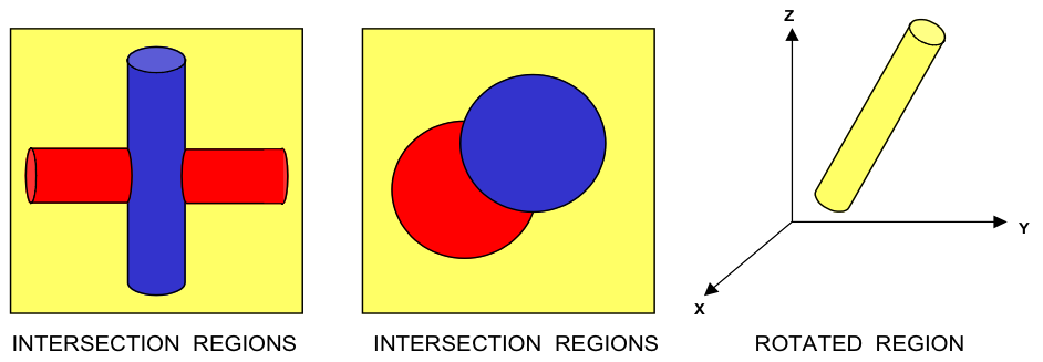
Fig. 8.1.1 Examples of geometry allowed in KENO-VI but not allowed in KENO V.a.

For KENO V.a, unless special options are invoked, each geometric region in a UNIT must completely enclose each interior region. Regions may touch at points of tangency and may share faces. See Fig. 8.1.2 for examples of allowable situations.

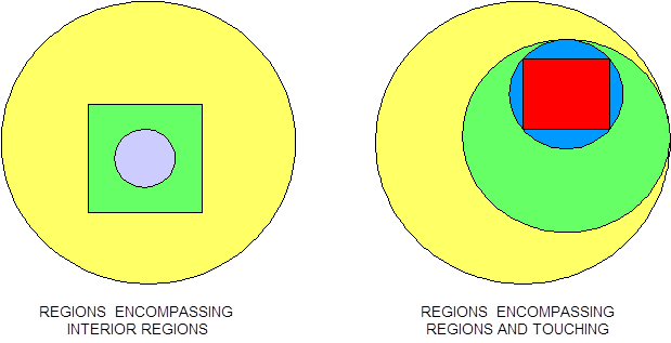
Fig. 8.1.2 Examples of correct KENO V.a units.

Special options are provided to circumvent the complete enclosure restriction in KENO V.a or to enhance the basic geometry package in KENO-VI. These options include ARRAY and HOLE descriptions. The HOLE option is the simplest of these and allows placing a UNIT anywhere within a region of another UNIT. In KENO V.a, HOLEs are not allowed to intersect the region into which they are placed; this restriction does not apply in KENO-VI (see Fig. 8.1.3). In both geometry packages, a HOLE cannot intersect the UNIT boundary. It is recommended that the outer boundary of a UNIT used as a HOLE should not be tangent to or share a boundary with another HOLE or a region of the UNIT containing the HOLE because the code may find that the regions are intersecting due to precision and round-off. Since a particle must check every region to determine its location within a UNIT, using HOLEs to contain complex sections of a problem may decrease the CPU time needed for the problem in KENO-VI. Inclusion of HOLEs increases run-time in KENO V.a, but in many cases cannot be avoided. An arbitrary number of HOLEs can be placed in a region in combination with a series of surrounding regions. The only restrictions on HOLEs are (1) when they are placed in a UNIT, they must be entirely contained within the UNIT, and (2) they cannot intersect other HOLEs or nested ARRAYs. HOLEs in KENO V.a cannot intersect an ARRAY; in KENO-VI, the HOLE cannot intersect the ARRAY boundary.

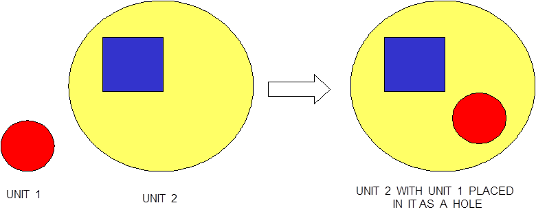
Fig. 8.1.3 Example demonstrating HOLE capability in KENO.

Lattices or arrays are created by stacking UNITs. In KENO V.a, only rectangular parallelepipeds can be organized in an ARRAY. HEXPRISMs and DODECAHEDRONs are allowed in KENO-VI to construct triangular pitched or closed-packed dodecahedral ARRAYs, respectively. The adjacent faces of adjacent UNITs stacked in this manner must match exactly. See Sect. 8.1.4.6.4 for additional clarification and Fig. 8.1.4 and Fig. 8.1.5 for typical examples.

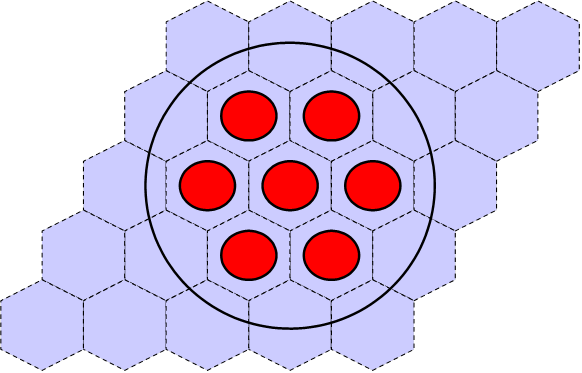
Fig. 8.1.4 Example of triangular pitched ARRAY construction.

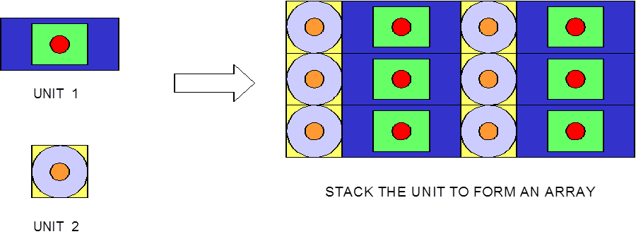
Fig. 8.1.5 Example of ARRAY construction.

The ARRAY option is provided to allow for placing an ARRAY or lattice within a UNIT. In KENO-VI, an ARRAY is placed in a UNIT by inserting it directly into a geometry/material region as a content record. In KENO V.a, the ARRAY is placed directly in the unit like a CUBOID: it must be the first region in the UNIT, or the ARRAY elements must intersect with the smaller region. Subsequent regions in the UNIT containing the ARRAY must contain it entirely. In KENO-VI, the reverse is true: the region boundary containing the ARRAY must coincide with or be contained within the ARRAY boundary. Therefore, in KENO-VI the region boundary becomes the ARRAY boundary, with the problem ignoring any part of the ARRAY outside the boundary. A particle enters or leaves the ARRAY when the region boundary is crossed. In KENO V.a, only one ARRAY can be placed directly in a UNIT. However, multiple ARRAYs can be placed within a UNIT by using HOLEs. When an ARRAY is placed in a UNIT via a HOLE, the UNIT that contains the ARRAY (rather than the ARRAY itself) is placed in the UNIT. ARRAYs of dissimilar ARRAYs can be created by stacking UNITs that contain ARRAYs. In KENO-VI, it is possible to place multiple ARRAYs in a UNIT by placing them in separate regions. Also in KENO-VI, using HOLEs to insert ARRAYs allows the ARRAYs to be rotated when placed. See Fig. 8.1.6 for an example of an ARRAY composed of UNITs containing HOLEs and ARRAYs.

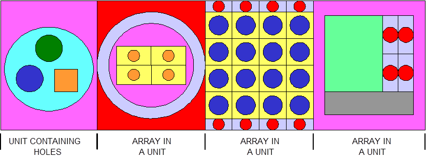
Fig. 8.1.6 Example of an ARRAY composed of UNITs containing ARRAYs and HOLEs.

The method of entering GEOMETRY_DATA in the geometry data block follows:

READ GEOM GEOMETRY_ DATA END GEOM

8.1.3.4.1.1. UNIT initialization

The description of a UNIT starts out with the UNIT INITIALIZATION and is terminated by encountering another UNIT INITIALIZATION or END GEOM.

The UNIT INITIALIZATION has the following format:

[GLOBAL] UNIT u

u is the identification number (positive integer) assigned to the particular UNIT. It may be used later to reference a UNIT previously constructed that the user wishes to place in a HOLE, or it may be used in an ARRAY (see below for more details).

GLOBAL is an attribute that specifies that the respective UNIT is the most comprehensive UNIT in the KENO problem to be solved, the UNIT that includes all the other UNITs and defines the overall geometric boundaries of the problem. In general, a GLOBAL UNIT must be entered for each problem.

Note

In KENO V.a, the GLOBAL specification is optional. If it is used, it can precede either a UNIT command or an ARRAY PLACEMENT_DESCRIPTION. If it is not entered and the problem does not contain ARRAY data, UNIT 1 is the default GLOBAL UNIT. If there is no GLOBAL UNIT specified and UNIT 1 is absent from the geometry description, an error message is printed. If the geometry description contains an ARRAY, KENO V.a defaults the global array to the array referenced by the last ARRAY PLACEMENT_DESCRIPTION that is not immediately preceded by a unit description. Otherwise, it is the largest array number specified in the array data (Sect. 8.1.3.5).

Examples of initiating a UNIT:

1. Initiate input data for UNIT No. 6.

UNIT 6

2. Initiate input data for the GLOBAL UNIT which is UNIT No. 4.

GLOBAL UNIT 4

For each UNIT, the UNIT’s DESCRIPTION follows the UNIT’s INITIALIZATION. The DESCRIPTION is realized by combining the commands listed below. The basic principles for constructing a UNIT are different between KENO V.a and KENO-VI. A brief discussion of these principles, together with a few examples, is presented at the end of this section following the description of the basic input used to build the geometry of a UNIT. The keywords that may be used to define a UNIT in KENO are as follows:

shape

COM=

HOLE

ARRAY

REPLICATE (KENO V.a only)

REFLECTOR (KENO V.a only)

MEDIA (KENO-VI only)

BOUNDARY (KENO-VI only)

8.1.3.4.1.2. Shape

Shape is a generic keyword used to describe a basic geometric shape that may be used in building the geometry of a particular UNIT. The general format varies between KENO V.a and KENO-VI. In KENO V.a, the shape defines a region containing a material, so the user is required to provide both a material and a bias ID. In KENO-VI the shape is used strictly as a surface, which is later used to define the mono-material regions (using the MEDIA card). The user is therefore required to enter a label for this surface so that the shape can be referenced later.

KENO V.a:

shape m b d₁ … d_N [a₁ …* [a_M ]…]

KENO-VI:

shape l d₁ … d_N [a₁ …* [a_M ]…]

shape is a generic keyword that describes a basic predefined KENO shape (e.g., CUBOID, CYLINDER) that is used to build the geometry of the UNIT. The predefined shapes differ between KENO V.a and KENO-VI. See Sect. 8.1.8.1 for a description of the KENO V.a basic shapes and Sect. 8.1.8.2 for the KENO-VI shapes.

m is the mixture number of the material (positive integer) that fills the particular shape in KENO V.a UNIT description. A material number of zero indicates a void region (i.e., no material is present in the volume defined by the shape).

b is the bias identification number (bias ID, a positive integer) assigned to the particular region defined by the shape in the KENO V.a UNIT description.

l is the label (positive integer) assigned to the particular shape in the KENO-VI UNIT description. This label is used later to define a certain mono-material region within the UNIT.

d₁ … d_N represent the N dimensions (floating point numbers) that define the particular shape (e.g., radius of a sphere or cylinder). See Sect. 8.1.8.1 and Sect. 8.1.8.2 for the particular value of N and how each shape is described.

a₁ … a_M are M optional ATTRIBUTES for the shape. The attributes provide additional flexibility in the shape description. The attributes that may be used with either KENO V.a or KENO-VI are described below (see shape ATTRIBUTES).

shape ATTRIBUTES

The ATTRIBUTES that can be used to enhance the shape description are CHORD, ORIG[IN], CENTER, and ROTATE (KENO-VI only).

The CHORD attribute

This attribute has different formats in KENO V.a and KENO-VI. The user will notice that it is more restrictive in KENO V.a. Only the HEMISPHERE and HEMICYLINDER shapes can be CHORDed in KENO V.a, but all 3-D shapes may be CHORDed in KENO-VI.

KENO V.a: CHORD \(\rho\)

KENO-VI: CHORD [+X=x+] [-X=x-] [+Y=y+] [-Y=y-] [+Z=z+] [-Z=z-]

\(p\) is the distance \(\rho\) from the cut surface to the center of the sphere

or the axis of a hemicylinder. See Fig. 8.1.7 and Fig. 8.1.8. Negative values of \(\rho\) indicate that less than half of the shape is retained, while positive values indicate that more than half of the shape will be retained.

+X=, -X=, +Y=, -Y=, +Z=, -Z=

are subordinate keywords that define the axis parallel to the chord. The “+” and “-” signs are used to define the side of the chord which is included in the volume. A “+” in the keyword indicates that the more positive side of the chord is included in the volume. A “-” in the keyword indicates that the more negative side of the chord is included in the volume.

x+, x-, y+, y-, z+, z-

are the coordinates of the plane perpendicular to the chord. For each chord added to a body, the keyword CHORD must be used, followed by one of the subordinate keywords and its dimension.

In KENO V.a, the CHORD attribute is applicable for only hemispherical and hemicylindrical shapes, not for SPHERE, XCYLINDER, YCYLINDER, CYLINDER, ZCYLINDER, CUBE, or CUBOID.

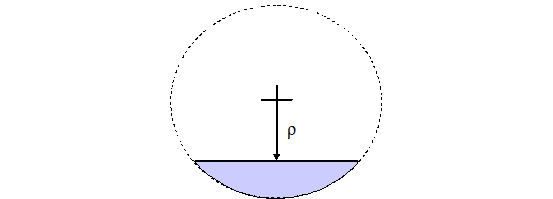
Fig. 8.1.7 Partial hemisphere or hemicylinder; less than half exists (less than half is defined by \(\rho < 0\)).

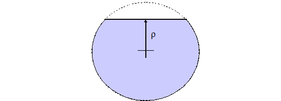
Fig. 8.1.8 Partial hemisphere of hemicylinder; more than half exists (more than half is defined by \(\rho > 0\)).

Fig. 8.1.9 provides two examples of the use of the CHORD option in KENO-VI.

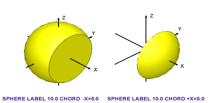
Fig. 8.1.9 Examples of the CHORD option in KENO-VI.

The ORIG[IN] attribute

The format is slightly different between KENO V.a and KENO-VI. Since the entries in KENO-VI are key worded, the user has more flexibility in choosing the order of these entries or in using default values. Only non-zero values must be entered in KENO-VI, but all applicable values, whether zero or non-zero, must be entered in KENO V.a.

KENO V.a: ORIG[IN] a b [c]

KENO-VI: ORIGIN [X=x₀] [Y=y₀] [Z=z₀]

\(a\)

is the X coordinate of the origin of a sphere or hemisphere; the X coordinate of the centerline of a Z or Y cylinder or hemicylinder; the Y coordinate of the centerline of an X cylinder or hemicylinder.

\(b\)

is the Y coordinate of the origin of a sphere or hemisphere; the Y coordinate of the centerline of a Z cylinder or hemicylinder; the Z coordinate of the centerline of an X or Y cylinder or hemicylinder.

\(c\)

is the Z coordinate of the origin of a sphere or hemisphere; it must be omitted for all cylinders or hemicylinders.

X=, Y=, Z=

are the subordinate keywords used to define the new position of the origin of the shape. If the a subordinate keyword appears more than once after the ORIGIN keyword, the values are summed. If the new value is zero, the particular coordinate does not need to be specified.

x₀, y₀, z₀

are the values for the new coordinates where the origin of the shape is to be translated.

The CENTER attribute

This attribute establishes the reference center for the flux moment calculations, which can be useful in TSUNAMI calculations. The syntax for this attribute is:

CENTER center_type [u] [x y z]

center_type

is the reference center value, as described in Table 8.1.18. The default value is global.

u

is the UNIT number to be used as a reference center for this region when the center_type is unit.

x, y, z

are the offset from the point specified by the center_type. The default is 0.0 for all three entries.

Table 8.1.18 Reference center values

center_type	Reference point
unit	Reference is defined as the origin of UNIT unit_number plus the offset defined by x, y, and z.
global	Reference is defined as system origin-i.e., (0,0,0) point of the GLOBAL UNIT-plus the offset defined by x, y, and z.
local	Reference is defined as the origin of the current UNIT plus the offset defined by x, y, and z.
fuelcenter	Reference is defined as the center of all fissile material in the system plus the offset defined by x, y, and z.
wholeunit	When entered for the first region in a unit, the reference for all regions in the unit are defined as the origin of the current unit plus the offset defined by x, y, and z.

The ROTATE attribute

This attribute can only be used in the KENO-VI input. It allows for the rotation of the shape or HOLE to which it is applied. If ORIGIN and ROTATE data follow the same shape or HOLE record, the shape is always rotated prior to translation, regardless of the order in which the data appear. Fig. 8.1.10 provides an example of the use of the ROTATE option. Its syntax is:

ROTATE [A1=a₁] [A2=a₂] [A3=a₃]

A1=, A2=, A3=

are subordinate keywords to specify the angles of rotation of the particular shape with respect to the origin of the coordinate system. The Euler X-convention is used for rotation.

a₁, a₂, a₃

are the values of the Euler rotation angles in degrees. The default is 0 degrees. If a subordinate keyword appears more than once following the ROTATE keyword, the values are summed.

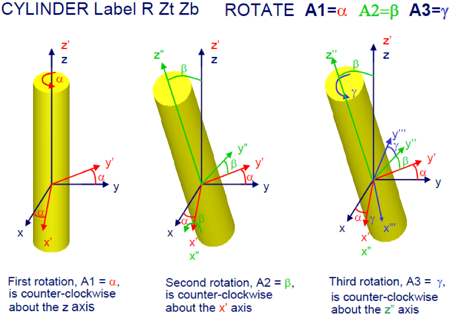
Fig. 8.1.10 Explanation of the ROTATE option.

Examples of shapes:

1. Specify a hemisphere labeled 10, containing material 2 with a radius of 5.0 cm which contains only material where Z > 2.0 within the sphere centered at the origin, and its origin translated to X=1.0, Y=1.5, and Z=3.0. KENO V.a (no label, but material and bias ID are the first two numerical entries):

   HEMISPHERE 2 1 5.0 CHORD -2.0 ORIGIN 1.0 1.5 3.0

   or

   HEMISPHE+Z 2 1 5.0 CHORD -2.0 ORIGIN 1.0 1.5 3.0

   KENO-VI (no material; this is to be specified with MEDIA):

   SPHERE 10 5.0 CHORD +Z=2.0 ORIGIN X=1.0 Y=1.5 Z=3.0

2. Specify a hemicylinder labeled 10, containing material 1, having a radius of 5.0 cm and a length extending from Z=2.0 cm to Z=7.0 cm. The hemicylinder has been truncated perpendicular to the X axis at X= -3 such that material 1 does not exist between X= -3 and X= -5. Position the origin of the truncated hemicylinder at X=10 cm and Y=15 cm with respect to the origin of the unit, and rotate it (in KENO-VI input) so it is in the YZ plane at X=10 and at a 45\(^{\circ}\) angle with the Y plane.

   KENO V.a (no rotation possible, no label):

   ZHEMICYL+X 1 1 5.0 7.0 2.0 CHORD 3.0 ORIGIN 10.0 15.0

   KENO-VI (no material; this is to be specified with MEDIA card):

   CYLINDER 10 5.0 7.0 2.0 CHORD +X= -3.0 ORIGIN X=10.0 Y=15.0 ROTATE A2= -45

8.1.3.4.1.3. COM=

The keyword COM= signals that a comment is to be read. The optional comment can be placed anywhere within a unit definition. Its syntax is:

COM = delim comment delim

delim

is the delimiter, which may be any one of ” , ` , * , ^ , or !

comment

is the comment string, up to 132 characters long.

Example of comment within a UNIT:

COM=”This is a fuel pin”

8.1.3.4.1.4. HOLE

This entry is used to position a UNIT within a surrounding UNIT relative to the origin of the surrounding UNIT. HOLEs may share surfaces with but may not intersect other HOLEs, the BOUNDARY of the UNIT which contains the HOLE, or an ARRAY boundary. In KENO-VI, the BOUNDARY record of a UNIT placed in a HOLE may contain more than one geometry label, but all labels must be positive, indicating inside the respective geometry bodies. The syntax for HOLE is:

KENO V.a: HOLE u x y z

KENO-VI: HOLE u [a₁ … [a_M ]…]

u

is the unit previously defined that is to be placed within the HOLE.

x y z

is the position of the HOLE in the KENO V.a host UNIT.

a1 … aM

are optional KENO-VI ATTRIBUTES for the HOLE. The ATTRIBUTES can be ORIGIN or ROTATE and follow the same syntax previously defined for KENO-VI shape ATTRIBUTES. These ATTRIBUTES allow for the translation and/or rotation of the HOLE within the host region.

Examples of HOLE use:

Place UNIT 2 in the surrounding UNIT such that the ORIGIN of UNIT 2 is at X=3, Y=3.5, Z=4 relative to the origin of the surrounding UNIT.

KENO V.a: HOLE 2 3 3.5 4

KENO-VI: HOLE 2 ORIGIN X=3.0 Y=3.5 Z=4.0

8.1.3.4.1.5. ARRAY

When used within a UNIT description, this entry provides an ARRAY placement description. In KENO V.a, it always starts a new UNIT and generates a rectangular parallelepiped that fits the outer boundaries of the specified ARRAY. The specified ARRAY is positioned in the UNIT according to the most negative point in the ARRAY with respect to the coordinate system of the surrounding UNIT. Thus, the location of the minimum x, minimum y, and minimum z point in the array is specified in the coordinate system of the UNIT into which the ARRAY is being placed.

In KENO-VI, the ARRAY keyword is used to position an ARRAY within a region in a surrounding UNIT relative to the origin of the surrounding UNIT. When the subordinate keyword PLACE is entered, it is followed by six numbers that precisely locate the ARRAY within the surrounding UNIT as shown in the example below. The first three numbers consist of the element in the ARRAY of the UNIT selected to position the ARRAY. The next three numbers consist of the position of the origin of the selected UNIT in the surrounding UNIT. Higher level ARRAY boundaries may intersect lower level ARRAY boundaries as long as they do not intersect HOLEs in the UNITs contained in the ARRAY or in UNITs contained in lower level ARRAYs.

The syntax for the ARRAY card is as follows:

KENO V.a: ARRAY array_id x y z

KENO-VI: ARRAY array_id l₁ … l_N [PLACE N_x N_y N_z x y z]

array_id

is the label that identifies the array to be placed.

l1 … lN

is the REGION DEFINITION VECTOR. These are previously defined shape labels, and together they define the region in which the array array_id is to be placed. This is used only in KENO-VI.

Nx Ny Nz

are three integers that define the element in the ARRAY of the UNIT selected to position the ARRAY. This is used only in KENO-VI.

x y z

specify the position of the ARRAY in the UNIT.

In KENO V.a, the x, y, and z values are the point where the most negative x, y, and z point of the ARRAY is to be located in the UNIT’s coordinates.

In KENO-VI, the x, y, and z values are the point where the origin of the UNIT specified by Nx, Ny, and Nz is to be located in the shape specified by the REGION DEFINITION VECTOR.

Example of ARRAY use:

In KENO V.a, position the most negative point of ARRAY 6 at X = 2.0, Y = 3.0, Z = 4.0 relative to the origin of the containing UNIT.

ARRAY 6 2.0 3.0 4.0

In KENO-VI, position instead the origin of UNIT (1,2,3) of ARRAY 6 at X = 2.0, Y = 3.0, Z = 4.0 and specify the ARRAY boundary to be the region that is inside the geometry shapes labeled 10 and 20 and outside the geometry shape labeled 30 used to describe the surrounding UNIT.

ARRAY 6 10 20 -30 PLACE 1 2 3 2.0 3.0 4.0

8.1.3.4.1.6. REPLICATE and REFLECTOR

These keywords specific to KENO V.a are used to generate additional geometry regions having the shape of the previous region. The geometry keyword REFLECTOR is a synonym for REPLICATE. The desired weighting functions can be applied to those regions by specifying biasing data as described in Sect. 8.1.3.7. The total thickness generated for each surface is the thickness per region for that surface times the number of regions to be generated, nreg.

The replicate specification is frequently used to generate weighting regions external to an ARRAY placement description. Thus an ARRAY placement description followed by a REPLICATE description would generate regions of a cuboidal shape. A cylindrical reflector could be generated by following the ARRAY placement description with a CYLINDER and then a REPLICATE. A HOLE cannot immediately follow a REPLICATE.

Extra regions using default weights can be generated by specifying the first importance region, imp, to be one that was not defined in the BIASING INFORMATION provided in a READ BIAS block. This capability can be used to generate extra regions for collecting information such as fluxes, leakage, etc.

Multiple replicate descriptions can be used in any problem. This capability can be used to model different reflector materials of different thicknesses on different faces.

The number of appropriate region dimensions needed for specifying REPLICATE is determined by the preceding region. For example, if the previous region were a SPHERE, one entry (i.e., t₁) would be required. If the previous region were a CYLINDER, the first entry, t₁, would be the thickness/region in the radial direction, the second entry, t₂, would the thickness/region in the positive length direction, the third entry, t₃, would be the thickness/region in the negative length direction, etc. The REPLICATE specification requirements for a CUBE are the same as for a CUBOID.

Syntax:

REPLICATE|REFLECTOR m b t₁ … t_N nreg

m

is the number of the material (non-negative integer) that fills the particular REPLICATE/REFLECTOR region in the UNIT description. A material of zero indicates a void region (i.e., no material is present in the volume defined by the shape).

b

is the bias identification number (positive integer) assigned to the particular region defined by the shape in the KENO V.a UNIT description. If the specified bias ID is defined in a READ BIAS block, the bias ID number will be incremented automatically, increasing one for each additional region up to nreg.

t₁ … t_N

represent the thickness (floating point number) per region for each of the N surfaces that define the particular shape. If the specified bias ID is one that is defined in the READ BIAS block, the region thicknesses should be consistent with the thicknesses used to generate the bias data being used. See Sect. 9.1.2.7.

nreg

is the number of regions (integer) to be generated.

Example:

Create five regions of material 4, each being 3 cm thick, outside a cuboid region (a cuboid has six dimensions). The inner-most of the five generated regions has a bias id of 2. The following four regions have bias id of 3, 4, 5, and 6.

8.1.3.4.1.7. MEDIA

This card is used in the KENO-VI input file to define the location of a mixture relative to the geometric shapes in the UNIT. Fig. 8.1.11 shows the input for a set of three intersecting SPHEREs in a CUBOID. The total volume data for a region in the problem may be entered as the last entry on the MEDIA card by using the VOL= keyword immediately followed by the volume in cm³. The volume entered is the volume of the region in the unit multiplied by the number of times the unit occurs in the problem minus any volume excluded from the problem by ARRAY boundaries and HOLEs. The volumes for any or all regions may be entered. If the volume is entered here, this value will be used even if volumes are also entered as a file or calculated (See Sect. 8.1.3.13). Volumes not entered will be determined by the input specified in the VOLUME DATA block. If no volume is supplied, the KENO-VI default volume of -1 will be used. This only affects volume-averaged quantities, i.e., not k_eff.

Syntax:

MEDIA m b l₁ … l_N [VOL = v]

m

is the material (positive integer or zero for vacuum) that fills the region defined by MEDIA.

b

is the bias id for the material sector being defined.

l₁ … l_N

is the region definition vector (N integers). These are N previously defined shape labels that together define the material sector.

VOL =

is an optional sub-keyword used to input the material sector volume.

v

is the volume in cm³ of the material sector defined by the MEDIA card.

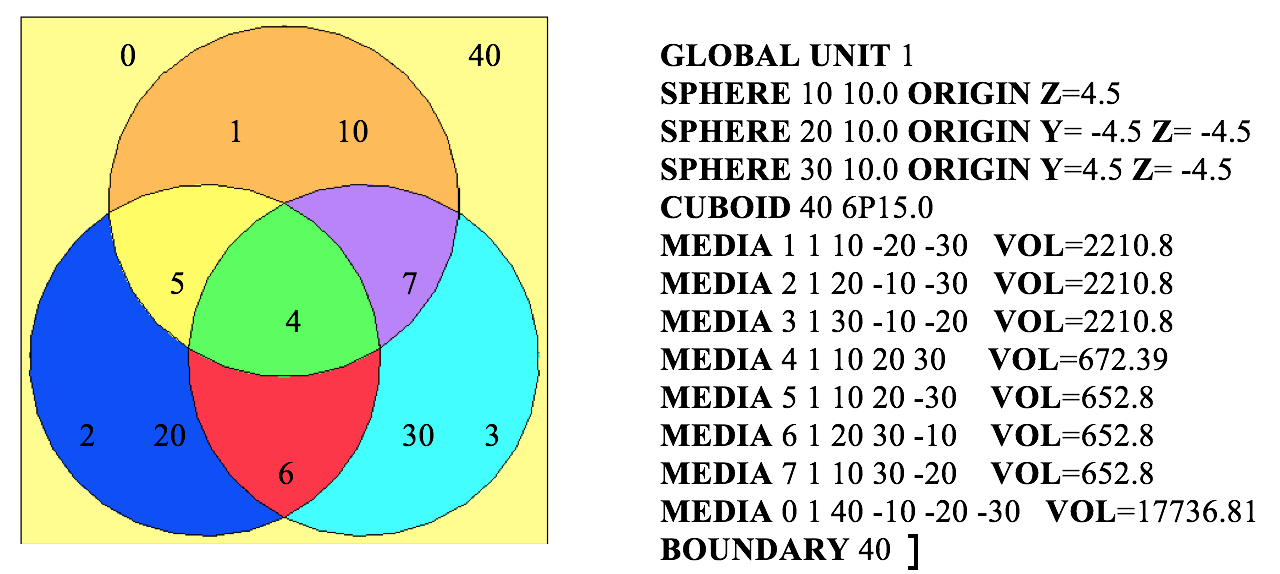
Fig. 8.1.11 Example of the MEDIA record.

8.1.3.4.1.8. BOUNDARY

This card is used in KENO-VI to define the outer boundary of the UNIT. In KENO V.a, the outer boundary of the UNIT is implicitly defined by the last shape in the UNIT. Each UNIT must have one and only one BOUNDARY card.

Syntax:

BOUNDARY l1 … lN

l₁ … l_N

is the UNIT BOUNDARY DEFINITION VECTOR (N integers). These are N previously defined shape labels that together define the outer boundary of the UNIT. All entries must be positive for the UNIT being defined to be used subsequently as a HOLE.

8.1.3.5. ARRAY Data

The array definition data block is used to define the size of an ARRAY and to position UNITs (defined in the geometry data) in a 3-D lattice that represents the ARRAY being described. As many arrays as are necessary can be described in a problem, subject to computer storage limitations. In KENO V.a, only one ARRAY may be placed directly in a UNIT, but as many ARRAYs as are needed may be placed in the UNIT by using HOLEs. In KENO-VI, any number of arrays can be placed in any UNIT either directly or indirectly using HOLEs. There is no default global array. If a global array is desired it must be explicitly defined.

The ARRAY definition data is entered as:

READ ARRAY ARRAY DATA END ARRAY

The ARRAY_ DATA consists of ARRAY_PARAMETERS and UNIT_ORIENTATION_DESCRIPTION.

8.1.3.5.1. ARRAY Parameters

The ARRAY parameters that can be used in the definition of an ARRAY are:

ARA=

GBL=

NUX=, NUY=, NUZ=

PRT=

COM=

TYP= (KENO-VI only)

8.1.3.5.1.1. ARA=

The ARA= parameter defines a reference number for an ARRAY. It has no default in KENO-VI. In KENO V.a, if is missing, the default is 1.

Syntax:

ARA=a

a

is the reference number for the ARRAY. It has no default in KENO-VI. In KENO V.a, if is missing, the default is 1.

8.1.3.5.1.2. GBL=

This is used to input the number of the global array.

Syntax:

GBL=g

g

is the reference number for the global ARRAY. In KENO V.a it must not be entered more than once. The default is the largest value for a, the reference number for the ARRAY. In KENO-VI it is no default value and if entered more than once, the last value is used.

8.1.3.5.1.3. PRT=

This entry is used to enable printing the ARRAY of UNIT numbers.

Syntax:

PRT=print

print

is a logical constant which defaults to YES, indicating that the ARRAY of UNIT numbers is printed. If the value is NO, then a summary table is printed instead containing the number of times each unit is used in each array.

8.1.3.5.1.4. NUX=, NUY=, NUZ=

These entries are used to input the number of units in the X, Y, and Z directions, respectively.

Syntax:

NUX=n_x NUY=n_y NUZ=n_z

n_x n_y n_z

are the number of units in the X, Y, and Z directions, respectively. There is no default in KENO-VI. In KENO V.a, each of them defaults to 1.

8.1.3.5.1.5. TYPE=

This entry is used to specify the type of ARRAY and is specific to KENO-VI, where more than one type of arrays can be used. It cannot be used in KENO V.a.

Syntax:

TYP=atyp

atyp

type of array (cuboidal or square, hexagonal or triangular, rhexagonal, shexagonal, dodecahedral), default = cuboidal

8.1.3.5.1.6. COM=

This keyword is used to enter a comment.

Syntax:

COM=delim comment delim

delim

is a delimiter. Acceptable delimiters are “, `, * , ^ , or !.

comment

is the comment string. Maximum comment length is 132 characters.

8.1.3.5.2. ARRAY orientation data

There are two methods to enter the UNIT numbers constituting an ARRAY: LOOP and FILL.

8.1.3.5.2.1. LOOP Construct

The LOOP construct resembles a FORTRAN DO-loop construct. The arrangement of UNITs may be considered as consisting of a 3-D matrix of UNIT numbers, with the UNIT position increasing in the positive X, Y, and Z directions, respectively.

Syntax:

LOOP u ix₁ ix₂ incx iy₁ iy₂ incy iz₁ iz₂ incz END LOOP

u

is the UNIT identification number (a positive integer).

ix₁

is the starting position in the X direction; ix₁ must be at least 1 and less than or equal to n_x of Sect. 8.1.3.5.1.4.

ix₂ is the ending position in the X direction; ix₂ must be at least 1 and less than or equal to nx.

incx

is the number of UNITs by which increments are made in the positive X direction; incx must be greater than zero and less than or equal to n_x.

iy₁

is the starting position in the Y direction; iy₁ must be at least 1 and less than or equal to n_y.

iy₂

is the ending position in the Y direction; iy₂ must be at least 1 and less than or equal to n_y.

incy

is the number of UNITs by which increments are made in the positive Y direction; incy must be greater than zero and less than or equal to n_y.

iz₁

is the starting position in the Z direction; iz₁ must be at least 1 and less than or equal to n_z.

iz₂

is the ending position in the Z direction;, iz₂ must be at least 1 and less than or equal to n_z.

incz

is the number of UNITs by which increments are made in the positive Z direction; incz must be greater than zero and less than or equal to n_z.

The syntax for ending the LOOP construct is:

END LOOP

The sequence u through incz is repeated until the entire ARRAY is described. If any portion of an ARRAY is defined in a conflicting manner, the last entry to define that portion will determine the ARRAY’s configuration. To use this feature, fill the entire ARRAY with the most relevant UNIT number and superimpose the other UNIT numbers in their proper places. An example showing the use of the LOOP option is given below. This 5 \(\times\) 4 \(\times\) 3 ARRAY of UNITs is a matrix of UNITs that has 5 UNITs stacked in the X direction, 4 UNITs in the Y direction, and 3 UNITs in the Z direction. X increases from left to right, and Y increases from bottom to top. Each Z layer is shown separately.

Given:

1 2 1 2 1         2 1 2 1 2       1 1 1 1 1
1 1 1 1 1         2 2 2 2 2       1 3 3 3 1
1 1 1 1 1         2 2 2 2 2       1 3 3 3 1
1 2 1 2 1         2 1 2 1 2       1 1 1 1 1
Z Layer 1         Z Layer 2       Z Layer 3

The data for this array could be entered using the following entries.

(1) 1 1 5 1 1 4 1 1 3 1 This fills the entire array with 1s.

(2) 2 2 5 2 1 4 3 1 1 1 This loads the four 2s in the first Z layer.

(3) 2 1 5 1 2 3 1 2 2 1 This loads the second and third rows of 2s in the second Z layer.

(4) 2 1 5 2 1 4 3 2 2 1 This loads the desired 2s in the first and fourth rows of the second Z layer.

(5) 3 2 4 1 2 3 1 3 3 1 This loads the 3s in the third Z layer and completes the array data input.

The second layer could have been defined by substituting the following data for entries (3) and (4):

(3) 2 1 5 1 1 4 1 2 2 1 This completely fills the second layer with 2s.

(4) 1 2 4 2 1 4 3 2 2 1 This loads the four 1s in the second layer.

When using the LOOP option, there is no single correct method of entering the data. If a UNIT is improperly positioned in the ARRAY or if some positions in the ARRAY are left undefined, it is often easier to add data to correctly define the ARRAY than to try to correct the existing data.

8.1.3.5.2.2. FILL Construct

The FILL construct enters data by stringing in UNIT numbers starting at X=1, Y=1, Z=1, and varying X, then Y, and then Z to fill the ARRAY. n_x x n_y x n_z entries are required. FIDO-like input options specified in Table 8.1.19 are also available for filling the ARRAY.

Syntax:

FILL u₁ … u_N {END FILL}|T

u₁ … u_N are the N=n_x x n_y x n_z UNIT numbers that make up the ARRAY

The syntax for ending the FILL construct is

END FILL

An alternative to end the UNIT data in FILL is by entering the letter T.

Table 8.1.19 FIDO-like input for mixed box orientation fill option.

Count field	Option field	Operand field	Function
		j	stores j at the current position in the array
i	R	j	stores j in the next i positions in the array
i	*	j	stores j in the next i positions in the array
i	$	j	stores j in the next i positions in the array
	F	j	fills the remainder of the array with unit number j, starting with the current position in the array
	A	j	sets the current position in the array to j
i	S		increments the current position in the array by i (This allows for skipping i positions; i may be positive or negative.)
i	Q	j	repeats the previous j entries i times (default value of i is 1)
i	N	j	repeats previous j entries i times, inverting the sequence each time. (default value of i is 1)
i	B	j	backs i entries. From that position, repeats the previous j entries in reverse order (default value of i is 1)
i	I	j k	provides the end points j and k, with i entries linearly interpolated between them (i.e., a total of i+2 points). At least one blank must separate j and k. When used for an integer array, the I option should only be used to generate integer steps-i.e., (k-j)/(i+1) should be a whole number
	T		terminates the data reading for the array

Note

When entering data using the options in this table, the count field and option field must be adjacent with no imbedded blanks. The operand field may be separated from the option field by one or more blanks.

Example: Consider a 3 \(\times\) 3 \(\times\) 1 ARRAY filled with 8 UNIT 1s and a UNIT 2, as shown below.

1     1       1
1     2       1
1     1       1

The input data to describe this ARRAY could be entered as follows:

Option (1) 1 1 1 1 2 1 1 1 1 T

This fills the array one position at a time, starting at the lower left corner. The T terminates the data.

or

Option (2) F1 A5 2 END FILL

The F1 fills the entire array with 1s, the A5 locates the fifth position in the array, and the 2 loads a 2 in that position. The END FILL terminates the data.

8.1.3.6. Albedo data

Albedo boundary conditions are entered using a FACE CODE to define where albedo conditions are to be used, and using an ALBEDO NAME to indicate which albedo condition is to be used on that face. The default value for each face is vacuum or void. The default values are overridden only on faces for which other albedo names are specified. Albedo boundary conditions are applied only to the outermost region of a problem (global boundaries). Different albedo options are allowed for different global boundaries, and this may show some differences in both KENO V.a and KENO-VI.

In previous SCALE versions, KENO V.a would have allowed the use of albedo boundary conditions to the boundary faces if and only if the outermost geometry region was a cuboid. For non-cuboidal outermost geometries, only the void or vacuum albedo option could have been applied. This limitation has been relaxed in SCALE 6.3; KENO V.a now allows some albedo options for non-cuboidal boundary shapes.

Unlike KENO V.a, KENO-VI allows a combination of geometry shapes to be used to define the boundaries of the global unit. Combinations of more than one geometry shape may result in re-entrant surfaces in the model. KENO-VI users need to be aware that when a neutron reaches a surface with a vacuum albedo, that neutron exits the model and the history ends. If a model contains features that are reentrant, that is a neutron could exit the model and reenter the model on the other side of an unmodeled region, all neutrons passing through the problem boundary are lost when they reach the unmodeled region. Neutrons are not “transported” across unmodeled areas between reentrant surfaces. It is not possible to create a KENO V.a model with reentrant problem outer boundary surfaces.

The syntax for entering the albedo boundary conditions is as follows. Note that BODY is no longer considered as a FACE CODE in the KENO-VI albedo boundary conditions capability, unlike the previous versions of SCALE.

KENO V.a:

READ BOUNDS fc₁=a₁ [fc₂=a₂]… [fc_N=a_N] END BOUNDS

KENO-VI:

READ BOUNDS [BODY=body_label ] fc₁=a₁ [fc₂=a₂]… [fc_N=a_N] END BOUNDS

fc₁ … fc_N are N FACE CODEs, each refers to a single or combination of multiple faces of the global boundaries (faces of the outermost region of a problem). FACE CODEs for different outer shapes are defined in Table 8.1.20.

a₁ … a_N are the ALBEDO NAMEs as defined in Table 8.1.23.

BODY= refers to the body or shape label in the global unit input. This optional parameter is available only for KENO-VI. The use of BODY with any face code combination is an optional feature for the problems in which the boundary definition vector of the global unit consists of a single body label (e.g. BOUNDARY 10). However, any face code used to specify an albedo condition on any face of a boundary shape must follow the BODY= parameter when the boundary definition vector of the global unit has more than one boundary labels (e.g., BOUNDARY 10 20 30). In such a case, all albedo boundary condition specifications following the BODY= definition are applied only on the faces of the body given with that BODY= definition.

body_label is the integer label of one of the shapes or bodies listed in the boundary definition vector of the global unit.

Albedo boundary conditions may be entered on each face of the global boundaries multiple times. The boundary condition that applies to the boundary face is the last one entered. If no boundary data are entered or if no albedo boundary condition is applied to a boundary face, then this boundary face is assumed to have a void or vacuum boundary condition. Similarly, albedo boundary conditions may be entered on each face of a boundary body listed in the boundary definition vector of the global unit multiple times. In this KENO-VI specific case, the boundary condition that applies to the boundary face of that body is the last one entered.

Example:

Apply the reflective albedo boundary condition to all faces of a cuboidal outer boundary except the positive X face.

In this sample problem, KENO with the ALL face code first applies the reflective albedo boundary condition to all faces of the outermost geometry. Then, the +XB= face code overrides the albedo type as VACUUM for the positive X face of the cuboidal outer boundary.

KENO V.a:

READ BOUNDS
   ALL=mirror +XB=vacuum
END BOUNDS

KENO-VI:

read geometry
   ...
   global unit 1
      CUBOID 10 ...
      ...
      BOUNDARY 10
end geometry

READ BOUNDS
   ALL=mirror +XB=vacuum
END BOUNDS

' following albedo specification is identical with the above one
' READ BOUNDS
'    BODY=10 ALL=mirror +XB=vacuum
' END BOUNDS

Example:

Apply a material-specific albedo H2O to all faces of the global boundaries except the bottom face of the cuboid, which is one of the boundary shapes. Another material-specific albedo CONC24 is applied to the bottom face of this cuboid.

This sample problem demonstrates the albedo boundary condition specification for a KENO-VI model in which outer boundary of the global unit is defined by a combination of a cuboid and a sphere (CUBOID 10 and SPHERE 20). KENO-VI, with this input, first applies a material-specific albedo, H2O, to all faces of BODY 10. Then, it overrides the boundary condition of the bottom face of the cuboid with another material-specific albedo, CONC24. Finally, material-specific albedo H2O is also applied to the spherical face of BODY 20.

KENO-VI:

read geometry
   ...
   global unit 1
      CUBOID 10 ...
      SPHERE 20 ...
      ...
      BOUNDARY 10 20
end geometry

READ BOUNDS
   BODY=10 ALL=H2O -ZB=CONC24
   BODY=20 ALL=H2O
END BOUNDS

' following albedo specification is identical with the above one
' READ BOUNDS
'    BODY=10 ALL=H2O
'    BODY=20 ALL=H2O
'    BODY=10 -ZB=CONC24
' END BOUNDS

All available FACE CODEs are described in Table 8.1.20. Note that the listed FACE CODEs are supported by both KENO V.a and KENO-VI.

Table 8.1.20 Face codes and surface numbers for entering boundary (albedo) conditions.

Face codes	Faces defined by face codes
ALL=	All faces of a single or multiple boundary shape(s)
SURFACE( k )=	Albedo surface enumeration indicates any \(k^{th}\) face of the boundary shape (Table 8.1.21 and Table 8.1.22 list shape-specific albedo surface numbers)
+XB=	Positive X face of a cuboidal boundary shape
&XB=	Positive X face of a cuboidal boundary shape
-XB=	Negative X face of a cuboidal boundary shape
+YB=	Positive Y face of a cuboidal boundary shape
&YB=	Positive Y face of a cuboidal boundary shape
-YB=	Negative Y face of a cuboidal boundary shape
+ZB=	Positive Z face of a cuboidal boundary shape
&ZB=	Positive Z face of a cuboidal boundary shape
-ZB=	Negative Z face of a cuboidal boundary shape
XFC=	Both positive and negative X faces of a cuboidal boundary shape
YFC=	Both positive and negative Y faces of a cuboidal boundary shape
ZFC=	Both positive and negative Z faces of a cuboidal boundary shape
+FC=	Positive X, Y, and Z faces faces of a cuboidal boundary shape
&FC=	Positive X, Y, and Z faces of a cuboidal boundary shape
-FC=	Negative X, Y, and Z faces of a cuboidal boundary shape
XYF=	Positive and negative X and Y faces of a cuboidal boundary shape
XZF=	Positive and negative X and Z faces of a cuboidal boundary shape
YZF=	Positive and negative Y and Z faces of a cuboidal boundary shape
+XY=	Positive X and Y faces of a cuboidal boundary shape
+YX=	Positive X and Y faces of a cuboidal boundary shape
&XY=	Positive X and Y faces of a cuboidal boundary shape
&YZ=	Positive X and Y faces of a cuboidal boundary shape
+XZ=	Positive X and Z faces of a cuboidal boundary shape
+ZX=	Positive X and Z faces of a cuboidal boundary shape
&XZ=	Positive X and Z faces of a cuboidal boundary shape
&ZX=	Positive X and Z faces of a cuboidal boundary shape
+YZ=	Positive Y and Z faces of a cuboidal boundary shape
+ZY=	Positive Y and Z faces of a cuboidal boundary shape
&YZ=	Positive Y and Z faces of a cuboidal boundary shape
&ZY=	Positive Y and Z faces of a cuboidal boundary shape
-XY=	Negative X and Y faces of a cuboidal boundary shape
-XZ=	Negative X and Z faces of a cuboidal boundary shape
-YZ=	Negative Y and Z faces of a cuboidal boundary shape
YXF=	Positive and negative X and Y faces of a cuboidal boundary shape
ZXF=	Positive and negative X and Z faces of a cuboidal boundary shape
ZYF=	Positive and negative Y and Z faces of a cuboidal boundary shape
-YX=	Negative X and Y faces of a cuboidal boundary shape
-ZX=	Negative X and Z faces of a cuboidal boundary shape
-ZY=	Negative Y and Z faces of a cuboidal boundary shape

Warning

In SCALE 6.3:

• Face codes, which are specific to the cuboidal boundary shape, cannot be used with non-cuboidal boundary shapes.

• SURFACE(..) face code cannot be used together with any cuboidal face codes listed in Table 8.1.20 if the outermost geometry is cube or cuboid.

• The ALL face code refers to all faces of the global boundaries.

Unlike the albedo boundary conditions capability in KENO codes of previous SCALE versions, FACE CODE definitions and their use are slightly different in SCALE 6.3.

SURFACE(..)= face code is a valid option for both KENO V.a and KENO-VI. SURFACE(..)= face code with a corresponding albedo surface number can be used to apply an albedo boundary condition to the specified surface of any boundary shape (cuboidal or non-cuboidal). Albedo surface enumerations for all geometric shapes supported by KENO V.a and KENO-VI are listed in Table 8.1.21 and Table 8.1.22, respectively. Note that entering an illegal albedo surface number with SURFACE(..) face code in bounds data input block fails the execution (i.e., SURFACE(2)=… for a sphere, SURFACE(9) for a hexprism, etc.)

The ALL= face code will apply the listed boundary condition to all surfaces of a single boundary shape, or multiple boundary shapes (KENO-VI only). It can be used with any boundary shape available in both KENO V.a and KENO-VI. If it follows a BODY= definition, then it refers to all the faces of the body given with that BODY= definition (KENO-VI only).

All the face codes, which are listed in Table 8.1.20, except ALL= and SURFACE(..), are specific to the cuboidal boundary shape, and they may be applied only to the cuboid or cube boundaries.

Table 8.1.21 Albedo surface numbers related to KENO V.a geometry shapes

GEOMETRY SHAPE	ALBEDO SURFACE ENUMERATION
	1	2	3	4	5	6
CUBE	+X	-X
CUBOID	+X	-X	+Y	-Y	+Z	-Z
CYLINDER	Radial	+Z	-Z
HEMISPHERE	Radial	Cut surface
HEMICYLINDER	Radial	Top	Bottom	Cut surface
SPHERE	Radial
XCYLINDER	Radial	+X	-X
YCYLINDER	Radial	+Y	-Y
ZCYLINDER	Radial	+Z	-Z

Table 8.1.22 Albedo surface numbers related to KENO-VI geometry bodies.

GEOMETRY BODY

ALBEDO SURFACE ENUMERATION

1

2

3

4

5

6

7

8

9

10

11

12

CONE

Radial

+Z

-Z

CUBOID

+X

-X

+Y

-Y

+Z

-Z

CYLINDER

Radial

+Z

-Z

DODECAHEDRON

+X

-X

+Y

-Y

+X +Y +Z

-X -Y -Z

-X +Y +Z

+X -Y -Z

-X -Y +Z

+X +Y -Z

+X -Y +Z

-X +Y -Z

ECYLINDER

Radial

+Z

-Z

ELLIPSOID

Radial

HEXPRISM

+X

-X

+X +Y

-X -Y

-X +Y

+X -Y

+Z

-Z

HOPPER

+X

-X

+Y

-Y

+Z

-Z

PENTAGON

-Y

+X -Y

+X +Y

-X +Y

-X -Y

+Z

-Z

PLANE

Surface

QUADRATIC

Surface

RHEXPRISM

+Y

-Y

-X +Y

+X -Y

+X +Y

-X -Y

+Z

-Z

RING

Inner Radius

Outer Radius

+Z

-Z

SPHERE

Radial

WEDGE

-Y

-X +Y

+X +Y

+Z

-Z

XCYLINDER

Radial

+X

-X

XPPLANE

+X

-X

YCYLINDER

Radial

+Y

-Y

YPPLANE

+Y

-Y

ZCYLINDER

Radial

+Z

-Z

ZPPLANE

+Z

-Z

Surfaces refer to the pre-rotation surface of the body that occurs in the indicated quadrant. Refer to Fig. 8.1.1 through Fig. 8.1.28 for illustrations of each geometry body.

All albedo names available in both KENO codes are given in Table 8.1.23. Table 8.1.23 lists also some material-specific albedo sets. Care must be exercised when using material-specific albedo types. These data sets were generated using a real problem, and they implicitly reflect the neutron energy spectrum, materials, and geometry from that model. Where neutron energy spectra, materials, and geometry vary from that model, the material-specific albedos may give significantly incorrect results. This may be checked by comparing results from a sample of calculations performed with both explicitly modeled reflectors and material-specific albedos. In general, use of material-specific albedos is not recommended.

Warning

The user should thoroughly understand material-specific albedos (e.g., DP0H2O, CON24, etc.) before attempting to use these reflectors. Misapplication of these problem-specific albedo data can cause the code to produce incorrect results without obvious symptoms.

Table 8.1.23 Albedo names available on the KENO albedo library for use with the face codes *

DP0H2O, DPOH2O, DP0, DPO	12 in. (30.48 cm) double P0 water differential albedo with 4 incident angles
H2O, WATER	12 in. (30.48 cm) water differential albedo with 4 incident angles
PARAFFIN, PARA, WAX	12 in. (30.48 cm) paraffin differential albedo with 4 incident angles
CARBON, GRAPHITE, C	78.74 in. (200.00 cm) carbon differential albedo with 4 incident angles
ETHYLENE, POLY, CH2	12 in. (30.48 cm) polyethylene differential albedo with 4 incident angles
CONC-4, CON4, CONC4	4 in. (10.16 cm) concrete differential albedo with 4 incident angles
CONC-8, CON8, CONC8	8 in. (20.32 cm) concrete differential albedo with 4 incident angles
CONC-12, CON12, CONC12	12 in. (30.48 cm) concrete differential albedo with 4 incident angles
CONC-16, CON16, CONC16	16 in. (40.64 cm) concrete differential albedo with 4 incident angles
CONC-24, CON24, CONC24	24 in. (60.96 cm) concrete differential albedo with 4 incident angles
VACUUM, VOID	Vacuum condition
SPECULAR, MIRROR, REFLECT	Mirror image reflection
PERIODIC	Periodic boundary condition
WHITE	White boundary condition
* Material-specific albedos (differential albedos) may not be used in continuous energy mode

Note

Differential albedos (material specific albedos), e.g., H2O and CONC, may not be used in continuous energy calculations. In multigroup mode, none of the differential albedos are allowed for the adjoint transport mode.

Different albedo options are allowed for different global boundaries. If the global boundary is a single cube or cuboids, then any available albedo option is allowed on any face of this cuboidal global boundary. However, if a periodic boundary condition is to be used, then it must be specified on opposing faces simultaneously.

Warning

There is no consistency check for the surfaces on which PERIODIC boundary condition has been specified. It is the user’s responsibility to specify the PERIODIC boundary condition on opposing faces simultaneously.

Albedo options for non-cuboidal global boundaries may show some differences in KENO V.a and KENO-VI:

KENO V.a:

• Albedo boundary conditions other than VACUUM are not allowed if the outermost geometry is either a hemisphere or a hemicylinder.

• Material-specific albedos cannot be applied to the curvilinear faces of the outermost geometry.

• MIRROR and PERIODIC boundary conditions are not allowed on the curvilinear faces of the outermost geometry.

• Whereas WHITE or VACUUM may be applied to the radial face of a cylinder, any albedo options can be used for the top and bottom faces.

Example:

Use a 24-in. concrete albedo boundary condition on the -Z face of the problem and use mirror image reflection on the +X and -X faces to represent an infinite linear array on a 2 ft thick concrete pad.

READ BOUNDS
   XFC=mirror -ZB=CONC24
END BOUNDS

Example:

A cylinder with arbitrarily chosen length is specularly reflected on the top and bottom faces to create an infinitely long cylinder.

READ BOUNDS
   SURFACE(2)=mirror SURFACE(3)=mirror
END BOUNDS

KENO-VI:

• Any CHORDed surfaces that are global unit boundaries will use the default (VOID) boundary condition, and this cannot be changed. Because KENO-VI does not provide any input method to assign a non-vacuum albedo boundary condition to the CHORDed surface(s), this restriction may need to be considered when building the geometry of the global unit.

• If the boundary definition vector of the global unit contains only a single body label, then all albedo boundary conditions are allowed on any face of the global boundary.

• If the boundary definition vector of the global unit contains multiple body labels and all these body labels are positive numbers (e.g. BOUNDARY 10 20 30), then all albedo boundary conditions may be applied to any of the faces of each body.

• If the boundary definition vector of the global unit contains multiple body labels and any of these body labels are negative numbers (e.g. BOUNDARY 10 20 -30), then only the VACUUM albedo is allowed on the faces of all bodies.

Caution

No non-vacuum albedo boundary conditions can be applied to a CHORDed surface that is global unit boundary.

Example:

A cylinder with an arbitrarily chosen length is specularly reflected on the top and bottom faces to create an infinitely long cylinder.

read geometry
   ...
   global unit 1
      CYLINDER 10 ...
      ...
      BOUNDARY 10
end geometry

READ BOUNDS
   ALL=mirror SURFACE(1)=void
END BOUNDS

' identical boundary condition can be applied with another definition
' READ BOUNDS
'    BODY=10 SURFACE(2)=reflective SURFACE(3)=mirror
' END BOUNDS

Example:

Use a 24 in. concrete albedo boundary condition on the -Z face of the problem and use mirror image reflection on the +X and -X faces to represent an infinite linear array on a 2 ft thick concrete pad.

read geometry
   ...
   global unit 1
      CUBOID 101 ...
      ...
      BOUNDARY 101
end geometry

READ BOUNDS
   SURFACE(1)=mirror SURFACE(2)=mirror SURFACE(6)=CON24
END BOUNDS

' identical boundary condition can be applied with another definition
' READ BOUNDS
'    BODY=101 XFC=reflective -ZB=CONC24
' END BOUNDS

Example:

Use a 24-in. concrete albedo boundary condition on the -Z face of a problem with a hexagonal boundary and use mirror image reflection on all side faces of the hexprism to represent an infinite planar array on a 2-ft-thick concrete pad.

read geometry
   ...
   global unit 1
      HEXPRISM 201 ...
      ...
      BOUNDARY 201
end geometry

READ BOUNDS
   SURFACE(1)=mirror SURFACE(2)=mirror
   SURFACE(3)=mirror SURFACE(4)=mirror
   SURFACE(5)=mirror SURFACE(6)=mirror
   SURFACE(7)=vacuum SURFACE(8)=conc24
END BOUNDS

' an alternative albedo specification for the same boundary conditions
' READ BOUNDS
'    ALL=mirror SURFACE(7)=vacuum SURFACE(8)=con24
' END BOUNDS
'

' an alternative albedo specification for the same boundary conditions
' READ BOUNDS
'    BODY=201 ALL=mirror SURFACE(7)=vacuum SURFACE(8)=con24
' END BOUNDS
'

' an alternative albedo specification for the same boundary conditions
' READ BOUNDS
'    ALL=mirror
'    BODY=201 SURFACE(7)=vacuum SURFACE(8)=con24
' END BOUNDS
'

Example:

The outer boundary of the global unit consists of a cuboid (body label 10) and a sphere (body label 20). The sphere is large enough to cut the corners of the cuboid leaving most of the cuboid intact. Use a 24 in. concrete albedo boundary condition on the -Z face of the cuboid to represent a 2 ft. thick concrete pad. Use the DP0H2O on the other surfaces to represent an infinite water reflector.

read geometry
   ...
   global unit 1
      CUBOID 10 ...
      SPHERE 20 ...
      ...
      BOUNDARY 10 20
end geometry

READ BOUNDS
   BODY=10 ALL=DP0H2O -ZB=CONC24
   BODY=20 SURFACE(1)=DPOH2O
END BOUNDS

' an alternative albedo specification for the same boundary conditions
' READ BOUNDS
'    ALL=DPOH2O
'    BODY=10 -ZB=CONC24
' END BOUNDS

Note that the ALL face code is used in two different ways in the above example: (1) Used with body 10 to apply DPOH2O albedo to all faces of this body (2) Used without body, which is legitimate for KENO-VI, to apply DPOH2O albedo to all faces of both body 10 and 20 (global unit boundaries defined by CUBOID 10 and SPHERE 20).

Example:

KENO geometry specification allows modeling the same physical problem with different geometry definitions. For some cases, boundary condition specification becomes more critical to represent the same problem with different geometry configurations. Users must be extra cautious when building their model and examine the limitations listed in this section carefully to prevent unexpected results.

This example was designed to demonstrate how ignoring such limitations for albedo boundary condition setup affects results in analysis. In this example, a model of a simplified version of a GODIVA sphere was attempted with three different geometry definitions as shown below.

KENO-VI, full GODIVA sphere:

...

READ GEOMETRY
   global unit 1
          sphere 30 8.75
      media 1 1 30
      boundary 30
END GEOMETRY

READ BOUNDS
   ALL=vacuum
END BOUNDS

KENO-VI, half GODIVA sphere defined by combination of a sphere and a cuboid:

...

READ GEOMETRY
   global unit 1
          sphere 30 8.75
      cuboid 40 8.75 0.0 4p8.75
      media 1 1 30 40
      boundary 30 40
END GEOMETRY

READ BOUNDS
   ALL=mirror
       BODY=30 surface(1)=void
END BOUNDS

KENO-VI, half GODIVA sphere defined by a sphere and a CHORD modifier:

...

READ GEOMETRY
   global unit 1
          sphere 30 8.75 chord +x=0.0
          media 1 1 30
          boundary 30
END GEOMETRY

READ BOUNDS
   ALL=mirror surface(1)=void
END BOUNDS

The first geometry definition uses only a sphere to define the Godiva sphere. The second sample input uses the combination of a sphere and a cuboid to define a hemisphere and an appropriate boundary condition on each outer boundary to simulate the Godiva sphere. Similarly, in the third sample input, a modified CHORD was used with a sphere to define a hemisphere and an appropriate boundary condition on each outer boundary to simulate the Godiva sphere.

But even if the sample input with the CHORDed surface given above seems correct at first glance, it cannot model the same physical problem as the other two because the albedo boundary condition specification with ALL=MIRROR is not applied to the CHORDed surface. Therefore, that CHORDed sphere models a half GODIVA sphere rather than a full one. Results from these three models, presented in Table 8.1.24, indicate that using code capabilities improperly might result in significant bias in the results.

Table 8.1.24 k-eff results of GODIVA models used in this example

Model	k-eff
Full sphere	1.02680 +/- 0.00100
Half sphere defined by a sphere and a cuboid	1.02962 +/- 0.00075
Half sphere defined by a sphere and a CHORD	0.78745 +/- 0.00078

Unlike KENO codes in previous versions, in SCALE 6.3, KENO codes print several warning messages to remind the user about such limitations and their potential effects if ignored.

Caution

There is no input method to assign a non-vacuum boundary condition to a CHORDed boundary surface (external boundary). Therefore, KENO-VI always applies VACUUM boundary condition to the CHORDed boundary surfaces, and this cannot be changed.

8.1.3.7. Biasing or weighting data

The biasing data block is used (in only multigroup mode) to define the weight that is given to a neutron surviving Russian roulette. The average weight of a neutron that survives Russian roulette, wtavg, is defaulted to dwtav (WTA= in the parameter data [see Sect. 8.1.3.3]) for all BIAS IDs and can be overridden by entering biasing information.

The biasing_information is used to relate a BIAS ID to the desired energy-dependent values of wtavg. This concept is similar to the way the MIXTURE ID, mat, is related to the macroscopic cross section data.

The weighting functions used in KENO  are energy-dependent values of wtavg that are applicable over a given thickness interval of a material. For example, the weighting function for water is composed of sets of energy-dependent values of wtavg for 11 intervals, each interval being 3 cm thick. The first set of wtavg’s is for the 0–3 cm interval of water, the second set of wtavg’s is for the 3–6 cm interval of water, etc. The eleventh set of wtavg’s is for the 30–33 cm interval of water.

To input biasing information, a BIAS ID must be assigned to correspond to a set of wtavg. Biasing data can specify a MATERIAL ID from the existing KENO V.a weighting library or from the AUXILIARY DATA input. The materials available from the KENO  weighting library are listed in Table 8.1.25.

The biasing_information is entered in one of the following two forms. The first set is said to input the CORRELATION DATA, while the second form is said to input the AUXILIARY DATA.

READ BIAS ID**\ =\ *m ib ie* ``END BIAS

or

READ BIAS WT[S]=wttitl id s t₁ i₁ g₁ w_1,1 … w_1,i1xg1 … t_s i_s g_s w_s,1 … w_s,isxgs END BIAS

ID= specifies that CORRELATION DATA will be entered next.

WT= or WTS= specifies that AUXILIARY DATA will be entered next.

m

is the identification (material ID) for the material whose weighting function is to be used. A material ID can be chosen from the existing KENO weighting library (Table 8.1.25) or from the auxiliary data input using the second form of the BIAS block as described later. If a material ID appears in both the KENO weighting library and the auxiliary data, the weights from the auxiliary data will be used.

ib

is the bias ID of the weighting function for the first interval of material m. The geometry record having the bias ID equal to ib will use the group-dependent weights from the first interval of material m.

ie

is the bias ID of the group-dependent weights from the (ie - ib + 1)th interval of material m.

wttitl

is an arbitrary title name (12 characters maximum), such as CONCRETE, WATER, SPECIALH2O, etc., to identify the material for which the user is entering data. Embedded blanks are not allowed.

id

is an identification number (material ID). The value is arbitrary. However, if the data are to be utilized in the problem, this ID must also be used at least once in the first form of the BIAS block.

s

is the number of sets of group structures for which weights will be read for this ID.

t₁… t_s

are s thicknesses of each increment for which weights will be read for this ID.

i₁… i_s

are s numbers of increments for which weights will be read for this ID.

g₁… g_s

are s numbers of energy groups for which weights will be read.

w_1,i1xg1… w_s,isxgs

are s sets of weights, each set containing a number of weights equal to the product of number of increments times the number of groups for that set. The group index varies the fastest.

Table 8.1.25 IDs, group structure and incremental thickness for weighting data available on the KENO  weighting library.

Material	Material ID	Group structure for which weights are available	Increment a thickness (cm)	Total number of increments available
Concrete	301	27 28 56 200 238 252	5 5 5 5 5 5	20 20 20 20 20 20
Paraffin	400	27 28 56 200 238 252	3 3 3 3 3 3	10 10 10 10 10 10
Water	500	27 28 56 200 238 252	3 3 3 3 3 3	10 10 10 10 10 10
Graphite	6100	27 28 56 200 238 252	20 20 20 20 20 20	10 10 10 10 10 10
a Group-dependent weight averages are supplied for each increment of the specified incremental thickness (i.e., for any given material) the first ngp (number of energy groups) weights apply to the first increment of the thickness specified here, the next ngp weights apply to the next increment of that thickness, etc CAUTION–If bias IDs defined in the weighting information data are used in the geometry, the region thickness should be consistent with the incremental thickness of the weighting data in order to avoiid overbiasing or underbiasing.

Warning

The user should thoroughly understand weighted tracking before attempting to generate and use auxiliary data for biasing. Incorrect weighting can cause the code to produce incorrect results without obvious symptoms.

Caution

1. Each set of AUXILIARY or CORRELATION data must be completely described in conjunction with its keyword. Complete sets of these data can be interspersed in an arbitrary order but data within each set must be entered in the specified order.

2. AUXILIARY DATA: If the same m is specified in more than one set of data, the last set having the group structure used in the problem is the set that will be utilized. When AUXILIARY DATA are entered, CORRELATION DATA must also be entered in order to use the AUXILIARY DATA.

3. CORRELATION DATA: If biasing data define the same bias ID (from the geometry data) more than once, the value that is entered last supersedes previous entries. Be well aware that multiple definitions for the same bias ID can cause erroneous answers due to overbiasing.

4. Bias data may not be used in continuous energy mode.

Examples

1. Use the first form of the BIAS block to utilize the water biasing factors in bias IDs 2 through 11. From Table 8.1.25, water has material ID m=500 and has bias parameters for 10 intervals that are each 3 cm thick.

READ BIAS ID=500 2 11 END BIAS

2. Use the second form of the BIAS block to specify biasing factors for SPECIALWATER to be used in bias IDs 6 and 7. The SPECIALWATER biasing factors have a value of 0.69 for BIAS ID 6 and 0.86 for bias ID 7 in each energy group. Sixteen-group cross sections are being used. Each weighting region is 3.048 cm thick. The material ID is arbitrarily chosen to be 510. Note that the first form of the BIAS block must be entered to allow the second form of the BIAS block to be used for BIAS IDs 6 and 7.

READ BIAS WT = SPECIALWATER 510 1 3.048 2 16 16*0.69 16*0.86 ID=510 6 7 END BIAS

3. An example of multiple definitions for the same bias ID follows:

READ BIAS ID=400 2 7 ID=500 5 7 END BIAS

The data for paraffin (ID=400) will be used for bias IDs 2, 3, and 4, and the data for water (ID=500) will be used for bias IDs 5, 6, and 7. The paraffin data for bias IDs 5, 6, and 7 have been overwritten by water data.

Multiple definitions for the same bias ID are not necessarily incorrect, but the user should be cautious about using multiple definitions and should ensure that the desired biasing or weighting functions are used in the desired geometry regions.

4. An example of how the bias ID relates to the energy-dependent values of weights is given below.

Assume that a paraffin reflector is to be used, and it is desirable to use the weighting function from the KENO weighting library to minimize the running time for the problem. Also assume that these weighting functions are to be used in the volumes defined in the geometry records having the bias ID (defined on a shape or MEDIA card for KENO V.a and KENO-VI, respectively) equal to 6, 7, 8, and 9. Correlation data are then entered and auxiliary data will not be entered.

The biasing data would be:

READ BIAS ID=400 6 9 END BIAS

The results of these data are

(1) the group-dependent weights for the 0–3 cm interval of paraffin will be used in the volume defined by the geometry region having bias ID= 6.

(2) the group-dependent weights for the 3–6 cm interval of paraffin will be used in the volume defined by the geometry region having bias ID= 7.

(3) the group-dependent weights for the 6–9 cm interval of paraffin will be used in the volume defined by the geometry region having bias ID= 8.

(4) the group-dependent weights for the 9–12 cm interval of paraffin will be used in the volume defined by the geometry region having bias ID= 9.

8.1.3.8. Start data

Special start options are available for controlling the initial neutron distribution. The default starting distribution for a global array is flat over the overall array dimensions, in fissile material only. The default starting distribution for a single unit is flat over the system, in fissile material only. See Table 8.1.26 for the starting distributions available in KENO. The syntax for the START block is:

READ START p1 …pN END START

p₁ …p_N are N initializations for the parameters listed below.

The starting information that can be entered is given below. Enter only the data necessary to describe the desired starting distribution.

NST = ntypst

start type, default = 0 Table 8.1.26 lists the available options under the heading, “Start type.”

TFX = tfx

the X coordinate of the point at which neutrons are to be started. Default = 0.0. Use for start types 3, 4, and 6.

TFY = tfy

the Y coordinate of the point at which neutrons are to be started. Default = 0.0. Use for start types 3, 4, and 6.

TFZ = tfz

the Z coordinate of the point at which neutrons are to be started. Default = 0.0. Use for start types 3, 4, and 6.

NXS = nbxs

the x index of the unit’s position in the global array. Default = 0. Use for start types 2, 3, and 6.

NYS = nbys

the y index of the unit’s position in the global array. Default = 0. Use for start types 2, 3, and 6.

NZS = nbzs

the z index of the unit’s position in the global array. Default = 0. Use for start types 2, 3, and 6.

KFS = kfis

the mixture whose fission spectrum is to be used for starting neutrons that are not in a fissionable medium. Defaulted to the fissionable mixture having the smallest mixture number. Available for start types 3, 4, and 6.

LNU = lfin

the final neutron to be started at a point. Default = 0. Each lfin should be greater than zero, and each successive lfin should be greater than the previous one. Use only for start type 6.

NBX = nboxst

the unit in which neutrons will be started. Default = 0. Use for start types 4 and 5.

FCT = fract

the fraction of neutrons that will be started as a spike or the relative fraction of each segment when using to specify a segmented distribution in z. Default = 0. Use for start type 2 and type 8.

XSM = xsm

the -X dimension of the cuboid in which the neutrons will be started. Default = 0.0. For an array problem, XSM is defaulted to the minimum X coordinate of the global array. If the outermost geometry is a cube or cuboid, then XSM is defaulted to the minimum X coordinate of this cuboid. Use for start types 0, 1, 2, 7, and 8.

XSP = xsp

the +X dimension of the cuboid in which the neutrons will be started. Default = 0.0. For an array problem, XSP is defaulted to the maximum X coordinate of the global array. If the outermost geometry is a cube or cuboid, then XSP is defaulted to the maximum X coordinate of this cuboid. Use for start types 0, 1, 2, 7, and 8.

YSM = ysm

the -Y dimension of the cuboid in which the neutrons will be started. Default = 0.0. For an array problem, YSM is defaulted to the minimum Y coordinate of the global array. If the outermost geometry is a cube or cuboid, then YSM is defaulted to the minimum Y coordinate of this cuboid. Use for start types 0, 1, 2, 7, and 8.

YSP = ysp

the +Y dimension of the cuboid in which the neutrons will be started. Default = 0.0. For an array problem, YSP is defaulted to the maximum Y coordinate of the global array. If the outermost geometry is a cube or cuboid, then YSP is defaulted to the maximum Y coordinate of this cuboid. Use for start types 0, 1, 2, 7, and 8.

ZSM = zsm

the -Z dimension of the cuboid in which the neutrons will be started. Default = 0.0 for only start types 0, 1, 2, and 7. For an array problem, ZSM is defaulted to the minimum Z coordinate of the global array. If the outermost geometry is a cube or cuboid, then ZSM is defaulted to the minimum Z coordinate of this cuboid. Use for start types 0, 1, 2, 7, and 8.

ZSP = zsp

the +Z dimension of the cuboid in which the neutrons will be started. Default = 0.0 for only start types 0, 1, 2, and 7. For an array problem, ZSP is defaulted to the maximum Z coordinate of the global array. If the outermost geometry is a cube or cuboid, then ZSP is defaulted to the minimum Z coordinate of this cuboid. Use for start types 0, 1, 2, 7, and 8.

RFL = rflkey

No longer supported (obsolete parameter).

PS6 = lprt6

the key for printing start type 6 input data. If the key is YES, then start type 6 data are printed. If it is NO, then start type 6 data are not printed. Enter YES or NO. Default = NO. Available for start type 6.

PSP = lpstp

the key for printing the neutron starting points using the tracking format. If the key is YES, then print the neutron starting points. If it is NO, then do not print the starting points. Enter YES or NO. Default = NO. Available for all start types.

RDU = rdu

the file from which ASCII start data are to be read for start type 6.

WS6 = ws6

the file to which the final fission neutron distribution from the last generation is written in ASCII start data format. Available for all start types. Initial neutron starting points from the first generation are also written in ASCII start data format to the file named initial_fission_neutrons_[ws6]. Both the initial and final neutron source distributions then can be viewed on a KENO geometry using the fission source viewer in Fulcrum.

MSS = filename.msl

the file from which ASCII start data are to be read. filename may include a valid pathname. Available for start type 9.

Note

All start types can write the initial neutron starting points at the last generation to an ASCII start data file specified by WS6. However, only start type 6 can read starting data from an ASCII start data file specified by RDU. The ASCII start data file format is described in Sect. 8.1.3.8.1.

Table 8.1.26 Starting distributions available in KENO.

Start type	Required data	Optional data	Starting distribution
0	None	NST XSM XSP YSM YSP ZSM ZSP PSP WS6 RFL a	Uniform throughout fissile material within the volume defined by (1) the outer region of a single unit, (2) the boundary of the global array, or (3) a cuboid specified by XSM, XSP, YSM, YSP, ZSM, and ZSP.
1	NST	XSM XSP YSM YSP ZSM ZSP PSP WS6 RFL a	The starting points are chosen according to a cosine distribution throughout the volume of a cuboid defined by XSM, XSP, YSM, YSP, ZSM, and ZSP. Points that are not in fissile material are discarded.
2	NST NXS NYS NZS FCT	XSM XSP YSM YSP ZSM ZSP PSP WS6 RFL a	An arbitrary fraction (FCT) of neutrons are started uniformly in the unit located at position NXS, NYS, NZS in the global array. The remainder of the neutrons is started in fissile material, from points chosen from a cosine distribution throughout the volume of a cuboid defined by XSM, XSP, YSM, YSP, ZSM, ZSP.
3	NST TFX TFY TFZ NXS NYS NZS	KFS PSP WS6	All neutrons are started at position TFX, TFY, TFZ within the unit located at position NXS, NYS, NZS in the global array.
4	NST TFX TFY TFZ NBX	KFS PSP WS6	All neutrons are started at position TFX, TFY, TFZ within units NBX in the global array.
5	NST NBX	PSP WS6	Neutrons are started uniformly in fissile material in units NBX in the global array.
6	NST TFX TFY TFZ LNU b	NXS NYS NZS KFS PS6 PSP RDU c WS6	The starting distribution is arbitrarily input. LNU is the final neutron to be started at a point TFX, TFY, TFZ relative to the global coordinate system or at a point TFX, TFY, TFZ, relative to the unit located at the global array position NXS, NYS, NZS.
7		XSM XSP YSM YSP ZSM ZSP PSP WS6	The starting points are chosen according to a flat distribution in the X- and Y-dimensions and a (1.0 - cos(z))2 distribution in the Z-dimension throughout the volume of a cuboid defined by XSM, XSP, YSM, YSP, ZSM, and ZSP. Points that are not in fissile material are discarded.
8	NST ZSM ZSP FCT	XSM XSP YSM YSP PSP WS6	Neutrons are started with flat distribution in X and Y, and a segmented distribution in Z, with the X-Y limits defined by XSM, XSP, YSM, YSP and the relative fraction in ZSP-ZSM defined by FCT. FCT must be the last entry for each segment.
9	NST MSS		Mesh source from Sourcerer d. The starting distribution is read from a previously created mesh source file declared with MSS=filename.msl, where filename may include a valid pathname.
a RFL parameter is no longer supported (obsolete parameter) b When entering data for start 6, LNU must be the last entry for each set of data, and the LNU in each successive set of data must be larger than the previous value of LNU. A set of data consists of required and optional data. c Starting points can be read from either a single or multiple ASCII start data file(s) specified with RDU. Each set of data with RDU must be followed by LNU that controls the number of starting points read from each file. Starting points read from an ASCII start data file can be also combined with any set of starting data specified with TFX/TFY/TFZ and/or NXS/NYS/NZS. d Sourcerer sequence has temporarily been removed from SCALE 6.3 because its design relied on legacy SCALE components. A new development has been in progress to redesign Sourcerer capability as a new START data type for both KENO and Shift transport codes, which will be available in next SCALE release.

Warning

Start data input block does not allow multiple start types defined together. Both KENO V.a and KENO-VI only process the start data entered in the first start data input block and discard the others if multiple start data input block defined in user input.

Example-1:

Both KENO V.a and KENO-VI read only start data from the first start data input block and ignore the second one. All starting points are uniformly sampled throughout the fissile materials iside the user-defined box (+x=3.0 -x=-3.0 +y= 1.0 -y=-1.0 +z= 2.0 -z=-2.0).

...

  READ START
     NST=0 XSP=3.0 XSM=-3.0 YSP=1.0 YSM=-1.0 ZSP=2.0 ZSM=-2.0
  END START

  READ START
     NST=6 TFX=2.0 TFY= 3.0 TFZ=0.0  LNU=25
  END START

end data
end

Optional parameters, XSM, XSP, YSM, YSP, ZSM, and ZSP allowed in start types 0, 1, 2, 7, and 8 are defaulted to 0.0. The default values are internally updated for the problems either with a global array or with a global unit with cuboid booundary shape as described above. User-defined values always override these defaults, and the last user entry always overrides the previous one. See Sect. 8.1.4.8 for details and more examples.

Note

User input specification with XSM > XSP or YSM > YSP or ZSM > ZSP is not considered as an error, and calculation is continued by swapping the values. Start type edit in output does not reflect the swapping operations.

Note

KENO-VI and KENO V.a has different interpretation for the source sampling when the user-defined cuboid is not inside the outermost geometry. In such a case, some starting points could be outside the global geometry, even though they are sampled inside the user-defined cuboid, and these points are considered as an error by KENO V.a; therefore, code terminates the execution after a couple errors have occurred. In contrast, rather than terminating execution, KENO-VI discards the points sampled outside the global geometry, and continues source sampling until all starting points have been sampled in the fissile regions inside the global unit.

Note

Unlike KENO V.a, the outer boundary can be any shape (or combination of shapes) in KENO-VI. For such a case, KENO-VI samples starting positions in the volume of the first body entered in the boundary definition vector of the global unit if and only if none of translation and transformation operations are performed on this body.

The start type 6 capability allows neutrons to be started at the arbitrary starting points defined by a set of data. The last entry for each start 6 data set must be LNU, and the LNU value of each successive set of data must be larger than the last. Start 6 data set with any of TFX, TFY, and TFZ, followed by LNU defines points relative to the global coordinate system, and with any of NXS, NYS, NZS, TFX, TFY, and TFZ followed by LNU defines points relative to the unit located at global array position (NXS, NYS, NZS).

In the start type 6 capabilitiy, TFX, TFY, and TFZ values are defaulted to 0.0, and NXS, NYS, and NZS values are defaulted to 0. This capability does not allow multiple entries of NXS, NYS, NZS, TFX, TFY, and TFZ in the same start 6 data set. NXS, NYS, NZS, TFX, TFY, and TFZ values entered in each start type 6 data set override their default values. A start type 6 data set with one or more missing TFX, TFY, and TFZ entries does not halt the execution. Instead, the last updated values of TFX, TFY, and TFZ are used for the missing one.

Start type 6 is capable of reading starting points from an ASCII start data file, which could be created by writing starting points from a previous calculation, defined by RDU in a start type 6 data set. See Sect. 8.1.3.8.1 for the details about a typical ASCII start data file currently supported, and Sect. 8.1.4.8 for more examples.

The following example was designed to illustrate the starting source distributions provided by start data types. Note that only start types 0, 1, 2, 5, 7, and 8 was used for this specific example.

Example-2:

In this example, a 2 \(\times\) 2 \(\times\) 1 rectangular array filled with four different units is used to demonstrate the different starting point distributions that can be generated by the starting types available in the start data capability. Spatial distribution of the starting points sampled with only start types 0, 1, 2, 5, 7, and 8 are overlayed on the problem geometry.

=kenovi
2x2 pin cell model for starting distribution demonstration
read parameters
   cep=ce_v7.1_endf gen=10  npg=5000 nsk=0 htm=no
end parameter

read mixt
   mix=1
      8016 3.91376E-02 92235 8.73674E-04 92238 1.87428E-02
   mix=2
      8016 3.91376E-02 92235 8.73674E-04 92238 1.87428E-02
   mix=31
     40090 2.17623E-02 40091 4.74582E-03 40092 7.25409E-03
     40094 7.35137E-03 40096 1.18434E-03
   mix=32
     40090 2.17623E-02 40091 4.74582E-03 40092 7.25409E-03
     40094 7.35137E-03 40096 1.18434E-03
   mix=41
     1001 4.77898E-02   1002 5.49646E-06  5010 4.75767E-06
     5011 1.91502E-05   8016 2.38396E-02  8017 9.08111E-06
   mix=42
     1001 4.77898E-02   1002 5.49646E-06  5010 4.75767E-06
     5011 1.91502E-05   8016 2.38396E-02  8017 9.08111E-06
end mixt

read geom
   unit   1
      com='UO2 Fuel Rod'
      cylinder 10   0.3860 6.0 0.0
      cylinder 20   0.4582 6.0 0.0
      cuboid   30 4p0.6375 6.0 0.0
      media  1 1 10
      media 31 1 20 -10
      media 41 1 30 -20
      boundary 30
   unit   2
      com='UO2 Fuel Rod'
      cylinder 10   0.3860 6.0 0.0
      cylinder 20   0.4582 6.0 0.0
      cuboid   30 4p0.6375 6.0 0.0
      media  2 1 10
      media 32 1 20 -10
      media 42 1 30 -20
      boundary 30
   unit   3
      com='UO2 Fuel Rod'
      cylinder 10   0.3860 6.0 0.0
      cylinder 20   0.4582 6.0 0.0
      cuboid   30 4p0.6375 6.0 0.0
      media  1 1 10
      media 31 1 20 -10
      media 41 1 30 -20
      boundary 30
   unit   4
      com='UO2 Fuel Rod'
      cylinder 10   0.3860 6.0 0.0
      cylinder 20   0.4582 6.0 0.0
      cuboid   30 4p0.6375 6.0 0.0
      media  2 1 10
      media 32 1 20 -10
      media 42 1 30 -20
      boundary 30
   global unit 5
      cuboid    10 4p1.275 6.0 0.0
      array  1  10 place 2 2 1  0.6375 0.6375  0.0
      boundary 10
end geom
read array
   ara=1 typ=square nux=2 nuy=2 nuz=1 gbl=1
      fill  1 3
            2 4
      end fill
end array
read bounds
   all=mirror
end bounds
end data
end

• start type 0 (default starting type), samples neutrons initial starting points uniformly throughout four fissile cylinders inside the global unit. Fig. 8.1.12 shows spatial distributions of the initial neutrons.

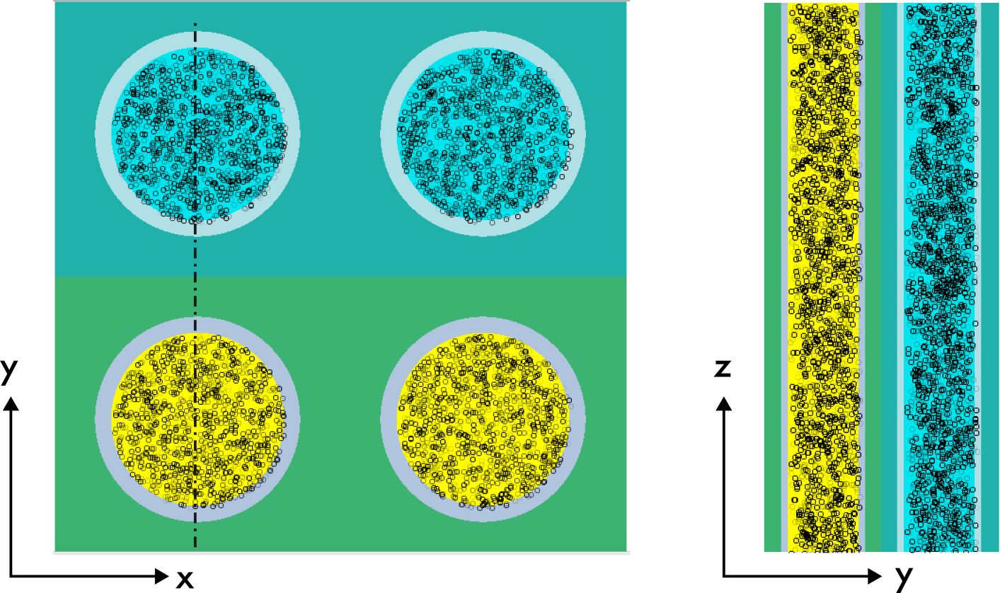
Fig. 8.1.12 Starting point distribution obtained with start type 0 overlayed on the geometry

Note

Overlaying starting distribution on Fulcrum-visualized geometry is now available in Fulcrum using the fission source viewer. Each of the fission source point overlays obtained using the WS6 option were generated using the fission source viewer with the geometry visualized in Fulcrum.

• start type 1, samples neutrons initial starting points with a cosine distribution (in each dimension) within a user-defined box given in start data input. All points except the ones in four fissile cylinders inside the global unit are discarded. Start type 1 produces initial neutron distributions concentrated in the middle of the problem as depicted in Fig. 8.1.13.

...

READ START
   NST=1 XSP=1.275 XSM=-1.275 YSP=1.275 YSM=-1.275 ZSP=6.0 ZSM=0.0
   PSP=YES WS6=keno1.src
END START

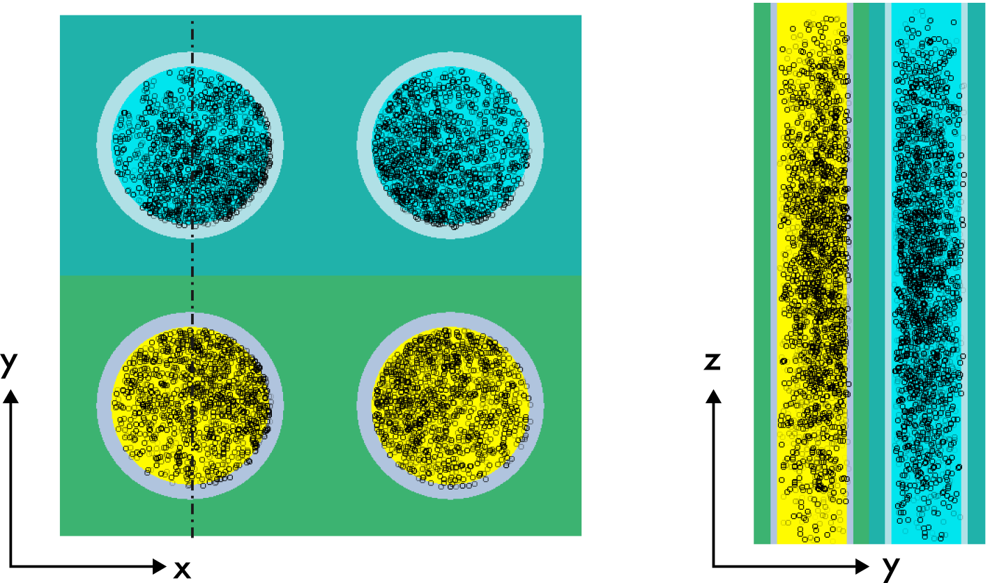
Fig. 8.1.13 Starting point distribution obtained with start type 1 overlayed on the geometry

• start type 2 is used with the array problems. With the following start data definition, an arbitrary fraction (FCT=0.5 in this case) of neutrons is started uniformly in the unit (unit=1) located at position NXS=1 NYS=1 and NZS=1 in the global array. The remainder of the neutrons are started in fissile material, from points chosen from a cosine distribution throughout the volume of a cuboid defined by +x=1.275 -x=-1.275 +y=1.275 -y=-1.275 +z=6.0 -z=0.0. All points except the ones in four fissile cylinders inside the user-defined cuboid are discarded. Start type 2 produces initial neutron distributions concentrated both in the middle of the problem and in the unit=1 located at the specified global array element. Fig. 8.1.14 shows both vertical and horizontal spatial distributions of the initial neutrons sampled with this start type.

...

READ START
   NST=2 XSP=1.275 XSM=-1.275 YSP=1.275 YSM=-1.275 ZSP=6.0 ZSM=0.0
   FCT=0.5 NXS=1 NYS=1 NZS=1
   PSP=YES WS6=keno2.src
END START

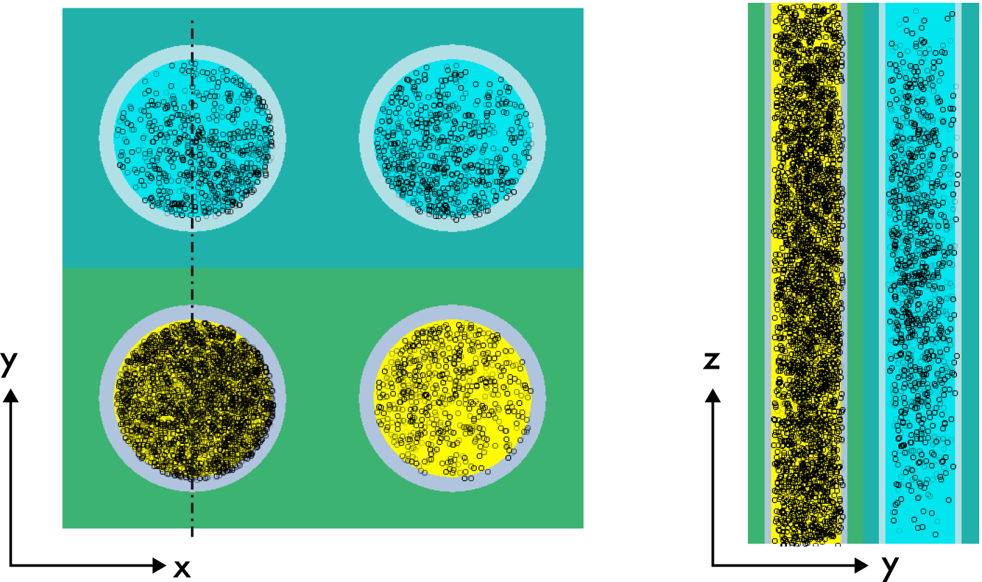
Fig. 8.1.14 Starting point distribution obtained with start type 2 overlayed on the geometry

• start type 5 uniformly samples initial starting points inside the unit=2 in the global array. Fig. 8.1.15 shows the both vertical and horizontal spatial distributions of the initial neutrons sampled with this start type.

...

READ START
   NST=5
   NBX=2
   PSP=YES WS6=keno5.src
END START

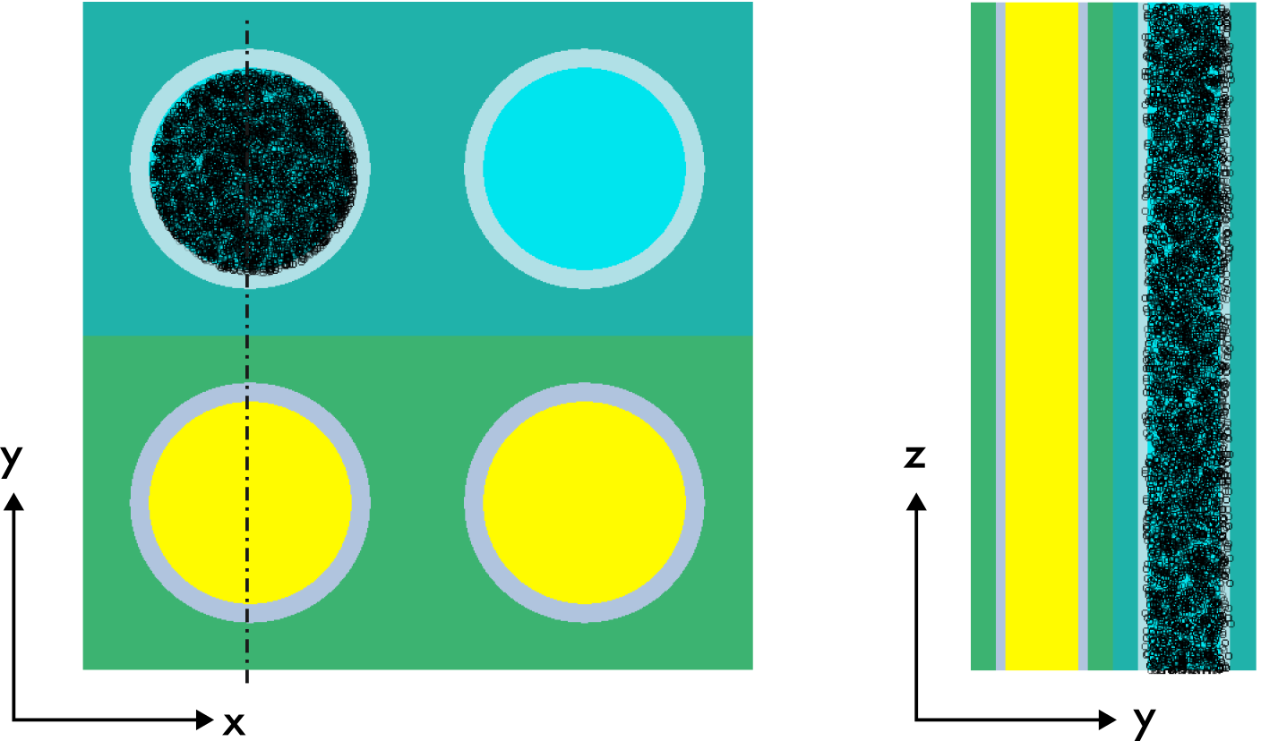
Fig. 8.1.15 Starting point distribution obtained with start type 5 overlayed on the geometry

• start type 7 samples neutrons initial starting points with a uniform distribution in X-Y and a \((1-cos)^2\) distribution in Z inside the cuboid defined by +x=1.275 -x=-1.275 +y=1.275 -y=-1.275 +z=6.0 -z=0.0. Start type 7 produces an initial neutron distributions concentrated to the top and bottom parts of the problem as shown in Fig. 8.1.16.

...

READ START
   NST=7 XSP=1.275 XSM=-1.275 YSP=1.275 YSM=-1.275  ZSP=6.0 ZSM=0.0
   PSP=YES WS6=keno7.src
END START

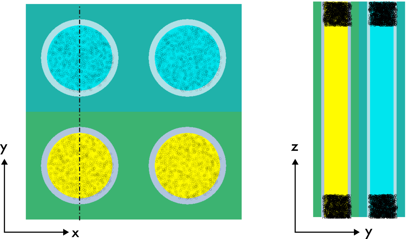
Fig. 8.1.16 Starting point distribution obtained with start type 7 overlayed on the geometry

• start type 8 samples the neutrons initial starting points with a uniform distribution in X-Y and a segmented distribution in Z inside the cuboid defined by +x=1.275 -x=-1.275 +y=1.275 -y=-1.275 +z=6.0 -z=0.0. Start type 8 with the specified input places the majority of the neutrons in the bottom of the problem and gradually decreases the neutron population from bottom to top using the user-provided segmented distribution as shown in Fig. 8.1.17.

...

READ START
   NST=8
   PSP=YES WS6=keno8.src
   XSP=1.275 XSM=-1.275 YSP=1.275 YSM=-1.275
   ZSM=0.0 ZSP=1.0 FCT=0.30
   ZSM=1.0 ZSP=2.0 FCT=0.25
   ZSM=2.0 ZSP=3.0 FCT=0.20
   ZSM=3.0 ZSP=4.0 FCT=0.13
   ZSM=4.0 ZSP=5.0 FCT=0.10
   ZSM=5.0 ZSP=6.0 FCT=0.02
END START

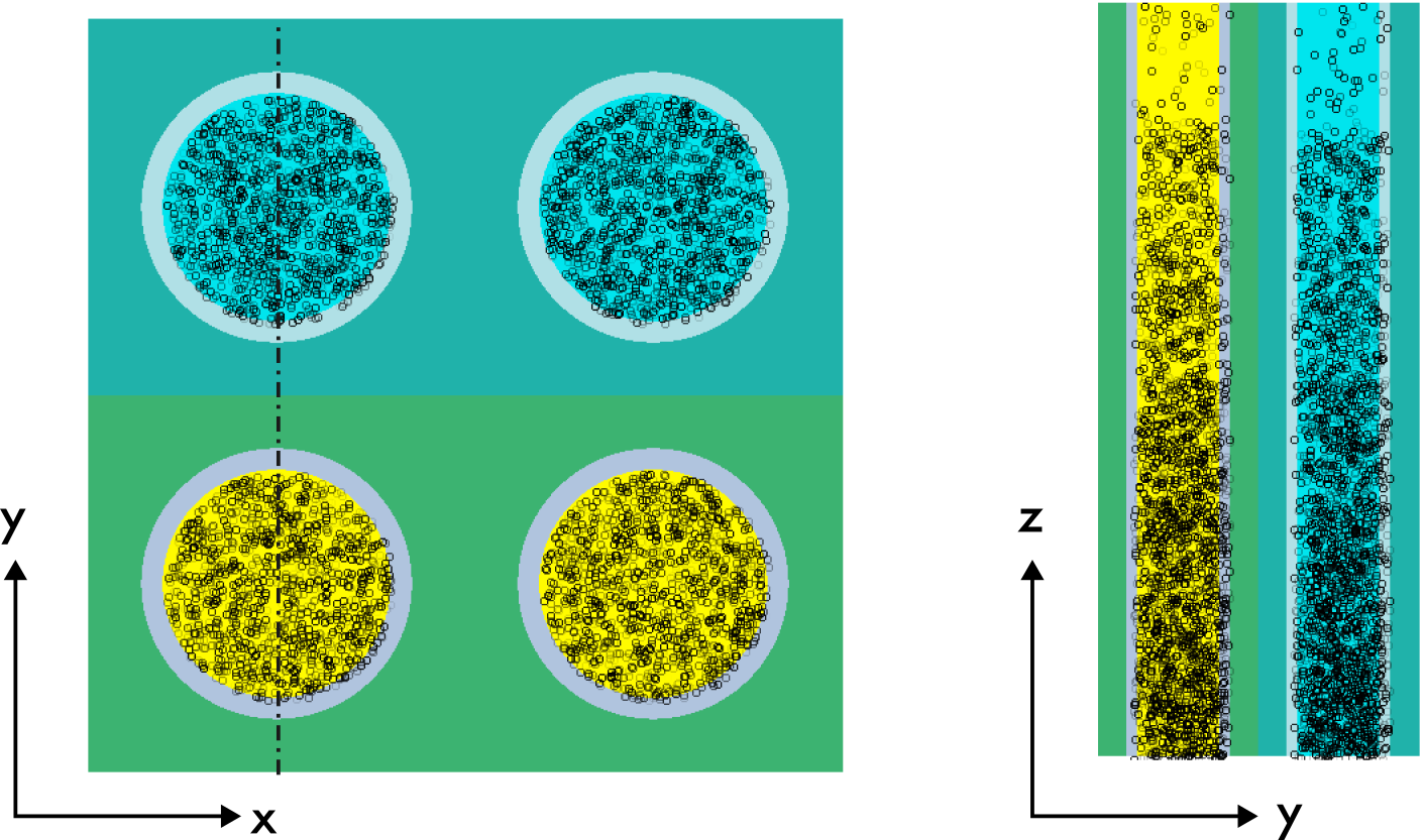
Fig. 8.1.17 Starting point distribution obtained with start type 8 overlayed on the geometry

8.1.3.8.1. ASCII Start Data File Format

A sample ASCII start data file is shown below. In a typical ASCII start data file, each line defines a data set. The first three columns are TFX, TFY, and TFZ values, the next four columns are NXS, NYS, NZS, and KFS, and the last column is always LNU. The file must be ended with a termination line with LNU =0. The file format is given with (3es20.9,5i12).

-1.000000000e-01    -2.000000000e+00    -3.300000000e+00           0           0           0         1           1
-3.000000000e-01    -2.400000000e+00    -3.300000000e+00           0           0           0         1          15
-3.000000000e-01    -2.500000000e+00    -3.300000000e+00           0           0           0         1          36
-4.000000000e-01    -2.600000000e+00    -3.300000000e+00           0           0           0         1          37
-4.000000000e-01    -2.700000000e+00    -3.300000000e+00           0           0           0         1          38
-5.000000000e-01    -2.800000000e+00    -3.300000000e+00           0           0           0         1          39
-5.000000000e-01    -2.900000000e+00    -3.300000000e+00           0           0           0         1          40
-5.000000000e-01    -2.900000000e+00    -3.300000000e+00           0           0           0         1           0

8.1.3.9. Extra 1-D XSECS IDs data

Extra 1-D cross section IDs are not required. They are allowed as input in order to simplify future modifications to calculate reaction rates, etc., as well as for compatibility with other SCALE codes. The syntax for the extra 1-D cross section data block is:

READ X1DS NEUTRON i1 …ix1d END X1DS

NEUTRON

is a keyword to indicate that the following ID identifies a neutron interaction.

i₁ … i_x1d

X1D 1-D identification numbers or keyword identifiers for the 1-D cross section to be used. These cross sections must be available on the mixture cross section library. X1D entries are expected to be read (see integer PARAMETER data).

8.1.3.10. Mixing table data

A cross section mixing table must be entered if KENO is being run stand alone and a Monte Carlo cross section format library is not being used in the multigroup mode, or KENO is being run stand alone in the continuous energy mode. If the parameter LIB= (Sect. 8.1.3.3) is entered, then mixing table data must be entered. A cross section mixing table is entered using the following syntax:

READ MIXT p₁ … p_N END MIXT

p₁ … p_N

are N parameters that might or might not be keyworded.

The possible parameters that can be used in a MIXT block are described below.

SCT = nsct

is used to input the number of scattering angles and only applies in multigroup mode. nsct is the number of discrete scattering angles, default = 1. The number of scattering angles specifies the number of discrete scattering angles to be used for the cross sections. If SCT is not set (i.e., SCT= -1), then the number of scattering angles is determined from the cross section library specified. The number of scattering angles defaults to (ncoef+1)/2, where ncoef is the largest Legendre polynomial order used in the problem. It needs to be entered only once for a problem. If more than one value is entered, the last one is used for the problem. For assistance in determining the number of discrete scattering angles for the cross sections, see Sect. 8.1.4.4.3.

EPS = pbxs

is used to enter the cross section message cutoff value, and it only applies in multigroup mode. pbxs is the value of the P₀ cross section for each transfer, above which generated warning messages will be printed, default = 3 × 10^-5. The primary purpose of entering this cutoff value is to suppress printing these messages when they are generated during cross section processing. For assistance in determining a value for EPS, see Sect. 8.1.4.4.4.

MIX = mix

is used to input the identification number of the mixture being described. mix defines the mixture being described.

NCM = ncmx

is used to input the nuclide mixture IDs to be used for this mixture. ncmx defines the nuclide mixture ID. When MIX=mix is read, ncmx is defaulted to mix also. Then, as long as all the nuclides that need to be mixed into mix already have mix specified as their nuclide mixture (frequently the case when using SCALE), the user does not need to specify NCM. The most usual case where NCM must be specified is when the mixtures were specified as a different mixture number when they were created in SCALE as compared to the mixture number used for them in KENO. Cell homogenized mixtures also need NCM specified.

TMP|TEM = temperature

is used to input the desired temperature of the CE cross section data.

nucl

is the nuclide ID number from the AMPX working format cross section library.

XS=fname

is used to input the optional continuous energy cross section filename to override the default cross sections. fname is the name of the file.

dens

is the number density (atoms/b-cm) associated with nuclide ID number nucl.

The sequence “nucl NCM=ncmx [XS=fname] dens” may be repeated until the mixture defined by MIX=mix has been completely described.

The sequence “MIX = mix NCM = ncmx TMP|TEM = temperature nucl NCM=ncmx [XS=fname] dens” may be repeated until all the mixtures have been described.

Note

If a given nuclide ID is entered more than once in the same mixture, then the number densities for that nuclide are summed.

If a mixture number is used as a nuclide ID, then it is treated as a nuclide and the number density associated with it is used as a density modifier. (If the density is entered as 1, then the mixture is mixed in at full density. If it is entered as 0.5, the mixture is mixed in at one half of its full density.) A Monte Carlo formatted cross section library is generated on the unit defined by the parameter XSC=. If this data set is saved, subsequent cases can utilize these mixtures without remixing.

The entry XS=fname is optional. If a nuclide is entered more than once in a mixture and this entry is specified, then they must be the same (i.e., cannot use more than one continuous energy cross section sets for a nuclide in a given mixture). Different mixtures may have the same nuclide with different continuous energy cross section sets.

8.1.3.11. Plot data

Plots of slices specified through the geometry can be generated and displayed (1) as character plots using alphanumeric characters to represent mixture numbers, unit numbers or bias ID numbers or (2) as color plots which generate a PNG file using colors to represent mixture numbers, unit numbers or bias ID numbers. Color plots require an independent program to display the PNG file to a PC or workstation monitor or to convert the file to be displayed using a plotting device. The keyword SCR= is used to control the plot display method. SCR=YES, the default value, uses the color plot display method. SCR=NO uses the character plot display method. The value of SCR determines the plot display method for all the plots specified in a problem. If SCR= is entered more than once, the last entry determines the plot display method. In other words, all plots generated by a problem will be either character plots or color plots.

The plot data can include the data for any or all types of plots. A plot by mixture number is the default. The kind of plot is defined by the parameter PIC=. Character plots are printed after the volumes are printed and before the final preparations for tracking are completed. Plot data are not required for a problem, but theyb can be used to verify the problem description. The actual plotting of the picture can be suppressed by entering PLT= NO in the parameter data or plot data. This allows plot data to be kept in the problem input for reference purposes without actually plotting the picture(s). Entering a value for PLT in the plot data will override any value entered in the parameter data. However, if a problem is restarted, the value of PLT from the parameter data is used. The upper left and lower right coordinates of the plot must be specified relative to the origin of the problem. See Sect. 8.1.4.10 for a discussion of plot origins and plot data.

Enter the plot data using the following syntax:

READ PLOT p₁ … p_N END PLOT

p₁ … p_N

are N parameters entered using keywords followed by the appropriate data. The plot title and the plot character string must be contained within delimiters. Enter as many picture parameters as necessary to describe the plot. Multiple sets of plot data can be entered. The parameter input for each plot is terminated by a labeled or unlabeled END. The labeled END cannot use the word PLOT as the first four characters of the label. For example, END PLT1 is a valid label, but END PLOT1 is not. If an unlabeled END is used, it cannot start in column 1.

The possible parameters that can be used in a PLOT block are described below.

TTL= delim ptitl delim

Enter a one-character delimiter delim to signal the beginning of the title (132 characters maximum). The title is terminated when delim is encountered the second time. Acceptable delimiters include ” , ` , * , ^ , or !. Default = title of the KENO case.

PIC= wrd The plot type, wrd, is followed by one or more blanks and must be one of the keywords listed below. The plot type is initialized to MAT; the default is the value from the previous plot.

MAT MIX[T[URE]] MEDI[A]	These keywords will cause the plot to represent the mixture numbers used in the specified geometry slice.
UNT UNIT[TYPE]	These keywords will cause the plot to represent the units used in the specified geometry slice. In the legend of the color plot, the material number actually refers to the units.
IMP BIAS[ID] WTS WEIG[HTS] WGT[S]	These keywords will cause the plot to represent the bias ID numbers used in the specified geometry slice. In the legend of the color plot, the material number actually refers to the bias ID numbers.

TYP =

Enter the type desired. XY for an X-Y plot XZ for an X-Z plot YZ for a Y-Z plot Direction cosines do not need to be entered if TYP is entered.

Plot coordinates

Enter values for the upper left and lower right coordinates of the plot as described below. Data must be entered for all nonzero coordinates unless all six values from the previous plot are to be used.

Upper left coordinates

Enter the X, Y, and Z coordinates of the upper left-hand corner of the plot.

XUL=xul

is used to enter the X coordinate of the upper left-hand corner of the plot. Default = value from previous plot; initialized to zero if any other coordinates are entered.

YUL=yul

is used to enter the Y coordinate of the upper left-hand corner of the plot. Default = value from previous plot; initialized to zero if any other coordinates are entered.

ZUL=zul

is used to enter the Z coordinate of the upper left-hand corner of the plot. Default = value from previous plot; initialized to zero if any other coordinates are entered.

Lower right coordinates

Enter the X, Y, and Z coordinates of the lower right-hand corner of the plot.

XLR=xlr

is used to enter the X coordinate of the lower right-hand corner of the plot. Default = value from previous plot; initialized to zero if any other coordinates are entered.

YLR=ylr

is used to enter the Y coordinate of the lower right-hand corner of the plot. Default = value from previous plot; initialized to zero if any other coordinates are entered.

ZLR=zlr

is used to enter the Z coordinate of the lower right-hand corner of the plot. Default = value from previous plot; initialized to zero if any other coordinates are entered.

Direction cosines across the plot

Enter direction numbers proportional to the direction cosines for the AX axis of the plot. The AX axis is from left to right across the plot. If any one of the AX direction cosines is entered, the other two are set to zero. The direction cosines are normalized by the code.

UAX=uax is used to enter the X component of the direction cosines for the AX axis of the plot. Default = value from previous plot; initialized to zero if any other direction cosines are entered.

VAX=vax is used to enter the Y component of the direction cosines for the AX axis of the plot. Default = value from previous plot; initialized to zero if any other direction cosines are entered.

WAX=wax is used to enter the Z component of the direction cosines for the AX axis of the plot. Default = value from previous plot; initialized to zero if any other direction cosines are entered.

Direction cosines down the plot

Enter direction numbers proportional to the direction cosines for the DN axis of the plot. The DN axis is from top to bottom down the plot. If any one of the DN direction cosines is entered, the other two are set to zero. The direction cosines are normalized by the code.

UDN=udn is used to enter the X component of the direction cosines for the DN axis of the plot. Default = value from previous plot; initialized to zero if any other direction cosines are entered.

VDN=vdn is used to enter the Y component of the direction cosines for the DN axis of the plot. Default = value from previous plot; initialized to zero if any other direction cosines are entered.

WDN=wdn is used to enter the Z component of the direction cosines for the DN axis of the plot. Default = value from previous plot; initialized to zero if any other direction cosines are entered.

Scaling parameters

Enter one or more scaling parameters to define the size of the plot.

Note

If any of the scaling parameters are entered for a plot, the value of those that were not entered is recalculated. If none of the scaling parameters are specified for a plot, the values from the previous plot are used.

DLX=dlx

is used to input the horizontal spacing between points on the plot. Default = value from previous plot; initialized to zero if NAX or NDN is entered.

DLD=dld

is used to input the vertical spacing between points on the plot. Default = value from previous plot; initialized to zero if NAX or NDN is entered.

Note

If either DLX or DLD is entered, the code will calculate the value of the other. If both are entered, the plot may be distorted.

NAX=nax

is used to input the number of intervals to be printed across the plot. Default = value from previous plot; initialized to zero if DLX or DLD is entered.

NDN=ndn

is used to input the number of intervals to be printed down the plot. Default = value from previous plot; initialized to zero if DLX or DLD is entered.

Global scaling parameter

LPI=lpi

is used to input a scaling factor used to control the horizontal to vertical proportionality of a plot or plots. SCALE 4.3 and later versions allow lpi to be input as a floating point number. For an undistorted character plot, lpi should be specified as the number of characters down the page that occupy the same distance as ten characters across the page. For an undistorted color plot, lpi should be entered as ten times the ratio of the vertical pixel dimension to the horizontal pixel dimension. The default value of lpi is 8.0 for a character plot and 10.0 for a color plot. lpi=10 will usually display an undistorted color plot.

The value entered for lpi applies to all plot data following it until a new value of lpi is specified.

Note

Plot data must include the specification of the upper left corner of the plot and the direction cosines across and down the plot.

Additional data required to generate a plot are one of the following combinations:

1. the lower right corner of the plot, the global scaling parameter, LPI, and one of the scaling parameters (DLX, DLD, NAX, NDN).

2. the lower right corner of the plot, one of the scaling parameters related to the horizontal specifications of the plot (DLX or NAX), and one of the scaling parameters related to the vertical specification of the plot (DLD or NDN). LPI, even if specified will not be used.

3. NAX and NDN and any two of LPI, DLX, and DLD. If LPI, DLX, and DLD are all specified, LPI is not used.

The data required to generate a plot may be supplied from (1) defaulted values, (2) data from the previous plot, or (3) data that are specifically entered for the current plot.

Miscellaneous parameters

Enter miscellaneous parameters

RUN=run

is used to determine if the problem is executed or is terminated after data checking. A value of YES for run means the problem will be executed if all the data were acceptable. A value of NO specifies the problem will be terminated after data checking is completed. The default value of RUN is YES.

PLT=plt

is used to specify if a plot is to be made. A value of YES for plt specifies that a plot is to be made. If plot data are entered, PLT is defaulted to YES.

Note

The parameters RUN and PLT can also be entered in the PARAMETER data. See Sect. 8.1.3.3. It is recommended that these parameters be entered only in the parameter data block in order to ensure that the data printed in the “Logical Parameters” table are what is actually performed.

SCR= src

This is used to determine the plot display method. The plot display method is specified by entering either YES or NO for src. The default value is YES. SCR=YES uses the color plot display method. SCR=NO uses the character plot display method. If SCR is entered more than once in a problem, the last value entered is the one that is used.

NCH= delim char delim

Enter only if plots are to be made utilizing the character plot display method (SCR=NO). Enter a delimiter (i.e., ” , ` , * , ^ , or !) to signal the beginning of character string char. The character string is terminated when the delim character is encountered the second time. Do not use the initial delimiter in the char string, as it will be read as terminating the string. char is a character string with each entry representing a plottable quantity (i.e., media {mixture} number, unit number, or bias ID). These are the characters that will be used in the plot. The first entry represents media, unit, or bias ID zero; the second entry represents the smallest media, unit, or bias ID used in the problem; the third entry represents the next larger media, unit, or bias ID used in the problem; etc. For example, assume PIC=MAT is specified, and 15 mixtures are defined in the mixing table, and the geometry data use only mixtures 3 and 7. By default, a blank will be printed for mixture zero, a 1 will be printed for mixture 3, and a 2 will be printed for mixture 7. If you wish to print a zero for a void (mixture 0), a 3 for mixture 3, and a 7 for mixture 7, enter NCH=`037’.

The default values of CHAR are the following:

Quantity	0	1	2	3	4	5	6	7	8	9	10	11	12	13	14	15
SYMBOL		1	2	3	4	5	6	7	8	9	A	B	C	D	E	F
Quantity	16	17	18	19	20	21	22	23	24	25	26	27	28	29	30	31
SYMBOL	G	H	I	J	K	L	M	N	O	P	Q	R	S	T	U	V
Quantity	32	33	34	35	36	37	38	39	40	41	42	43	44	45	46
SYMBOL	W	X	Y	Z	#	,	$	-	+	)		&	>	:	;
Quantity	47	48	49	50	51	52	53	54	55	56	57	58
SYMBOL	\(\cdot\)	-	“%”	“*”	“”“	“=”	“!”	“(“	“@”	“<”	“/”	0

CLR= n₁ r*(*n₁) g*(*n₁) b*(*n₁) … n_N r*(*n_N) g*(*n_N) b*(*n_N) END COLOR

this entry is used to define the colors to be used by the color plot. It may be entered only if plots are to be made utilizing the color plot display method (SCR=YES). After entering the keyword CLR=, 4 numbers are entered N times. The first number, n₁, represents a media (mixture) number, unit number, or bias ID. The next three numbers, whose values can range from 0 through 255, define the red, green, and blue components of the color that will represent this n₁ in the plot. The sequence of 4 numbers is repeated until the colors associated with all of the media (mixture) numbers, unit numbers, or bias IDs used in the problem have been defined. The smallest number that can be entered for n_i is -1, representing undefined regions in the plot. An ni of 0 represents void regions; n_i of 1 represents the smallest media, unit, or bias ID used in the problem; n_i of 2 represents the next larger media, unit, or bias ID used in the problem, etc. The color plot definition data are terminated by entering the keywords END COLOR. A total of 256 default colors are provided in Table 8.1.27 Two of those colors represent undefined regions, n_i=-1*, as black and void regions, and n_i=0 as gray. The remaining 254 colors represent the default values for mixtures, bias IDs, or unit numbers used in the problem. If num is entered as -1, the next three numbers define the color that will be used to represent undefined regions of the plot. The default color for undefined regions is black, represented as 0 0 0. If n_i is entered as 0, the next three numbers define the color that will represent void regions in the plot. The default color for void is gray, represented as 200 200 200. For example, assume a color plot is to be made for a problem that uses void regions and mixture numbers 1, 3, and 5. By default, the undefined regions (Index -1) will be black; void regions (Index 0) will be gray; the first mixture, mixture 1 (Index 1), will be medium blue; the next larger mixture, mixture 3 (Index 2), will be turquoise2; and the last mixture, mixture 5 (Index 3), will be green2. If these values are acceptable, data do not need to be entered for CLR=. If the user decides to define void to be white (255 255 255), mixture 1 to be red (255 0 0), mixture 3 to be bright blue (0 0 255), and mixture 5 to be green (0 255 0), then the following data could be entered:

CLR=0 255 255 255 1 255 0 0 2 0 0 255 3 0 255 0 END COLOR

In this example, the first number (0) defines the void, and the next three numbers are the red, green, and blue components that combine as the color white. The fifth number (1) represents the smallest mixture number (mixture 1), and the next three numbers are the red, green, and blue components of red. The ninth number (2) represents the next larger mixture number (mixture 3), and the next three numbers are the red, green, and blue components of bright blue. The thirteenth number (3) represents the next larger mixture number (mixture 5), and the next three numbers are the red, green, and blue components of green. The END COLOR terminates the color definition data. Because color data were not entered for ni of -1, undefined regions will be represented by the color black, the default specification from Table 8.1.27. The red, green, and blue components of some bright colors are listed below.

Display Color	red	green	blue
black	0	0	0
white	255	255	255
“default void gray”	200	200	200
red	255	0	0
green	0	255	0
brightest blue	0	0	255
yellow	255	255	0
brightest cyan	0	255	255
magenta	255	0	255

The 256 default colors are listed in Table 8.1.27.

Table 8.1.27 Default color specifications for the color plot display method

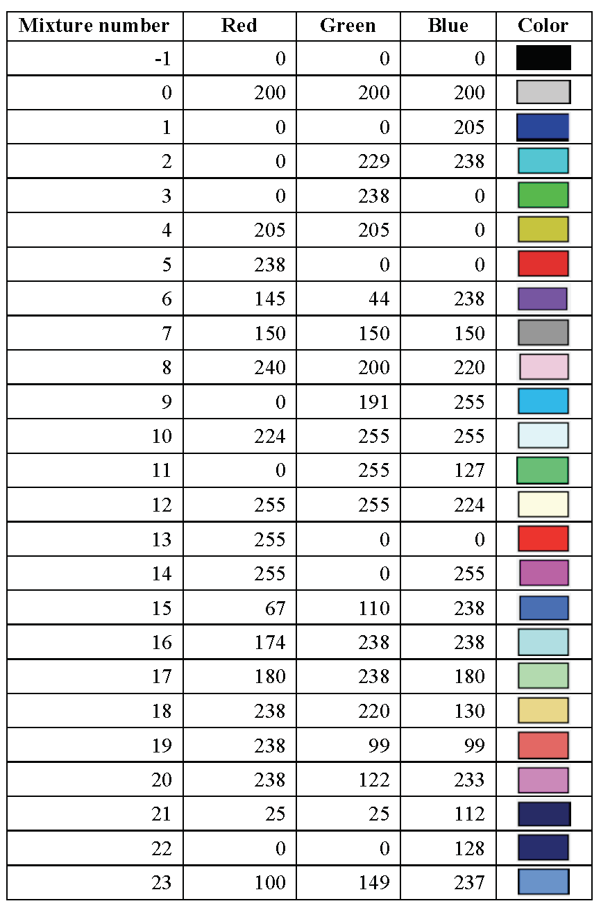
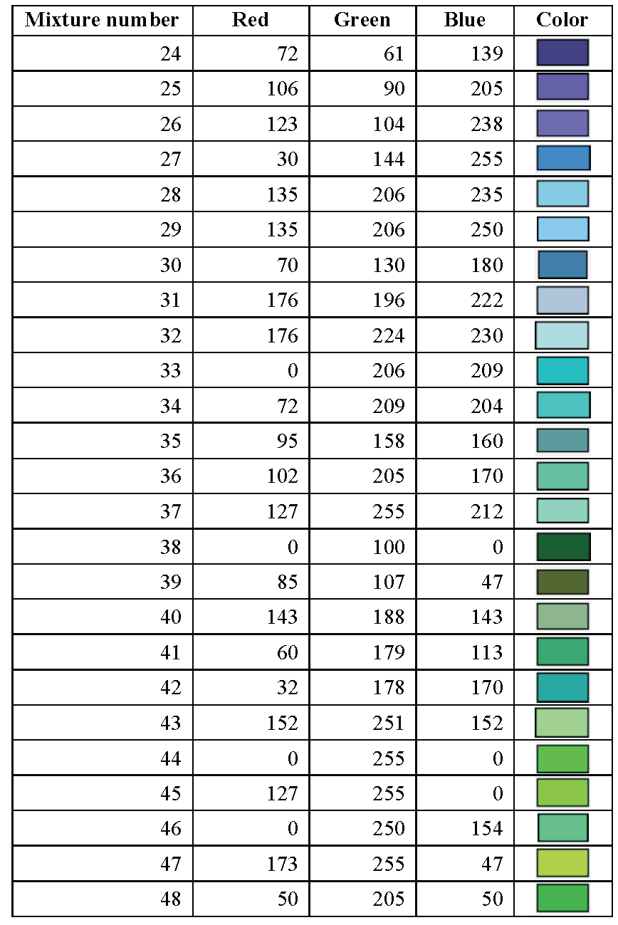
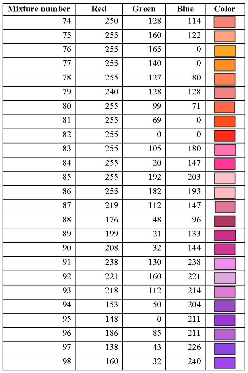
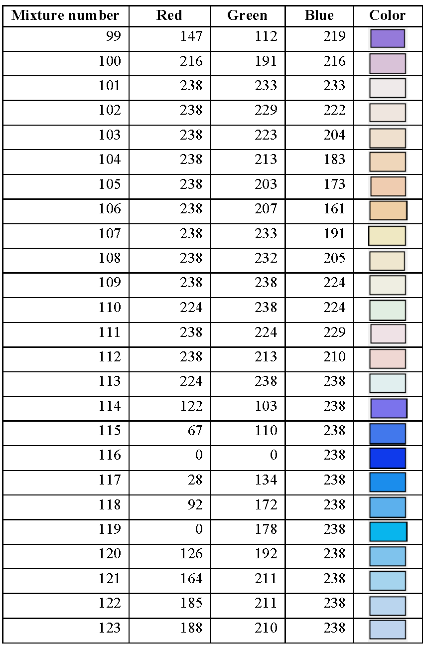
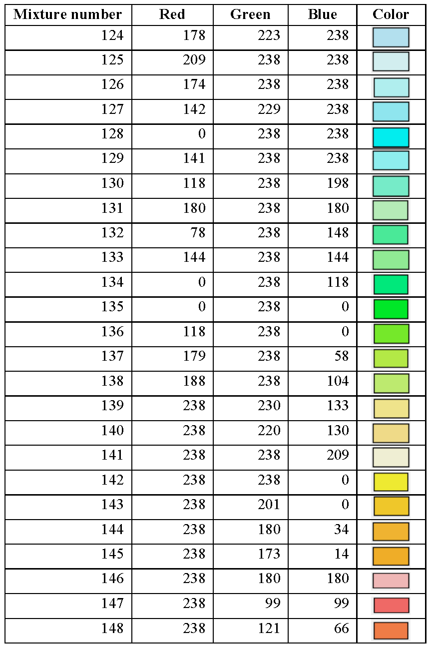
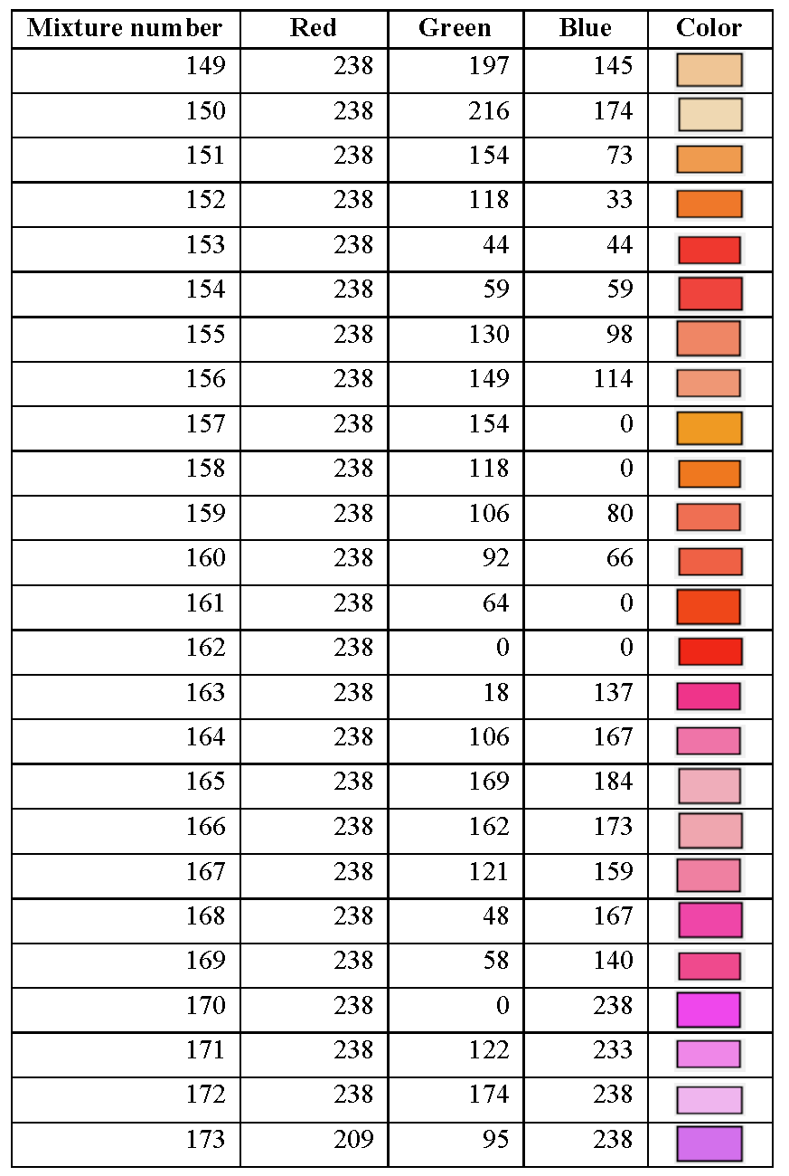
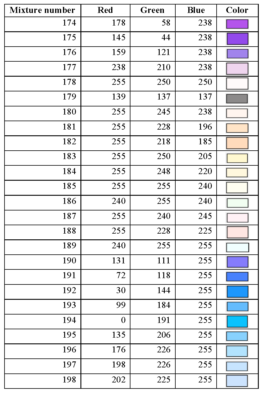
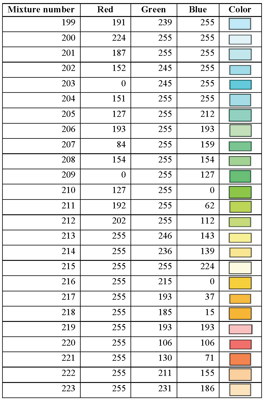
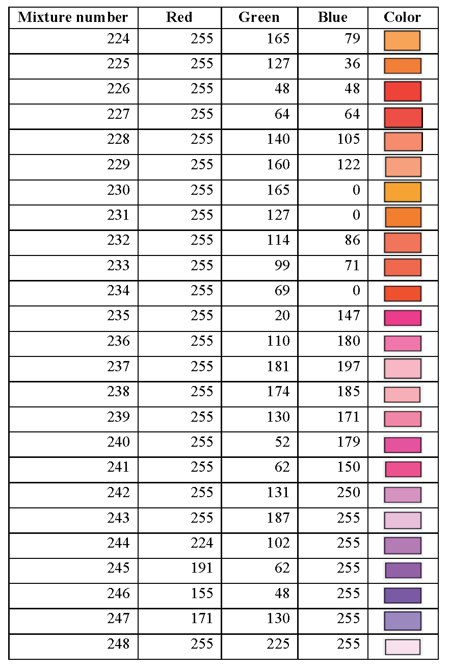
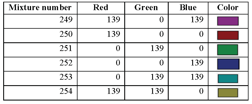
8.1.3.12. Energy group boundary data

Upper energy group boundary data in eV are entered to determine the groups into which the tallies will be collected in the continuous energy mode. For G groups G+1 entries are entered. The last entry is the lower energy boundary of the last group. The values must be in descending order. The parameter NGP is set equal to the number of entries-1. The syntax is:

READ ENERGY u₁ …uG u_G+1 END ENERGY

u₁ … u_G

are the upper energy limits of energy groups 1 … G, respectively.

u_G+1

is the lower energy limit of energy group G.

Example:

READ ENERGY

2e7 1e5 1 1e-5

END ENERGY

Defines a 3-group structure with group 1 (2e+7 eV to 1e+5 eV), group 2 (1e+5 eV to 1 eV), and group 3 (1 eV to 1e-5 eV) and sets NGP=3.

Energy group boundary data are optional. Default values for the energy group boundaries in the calculations are determined as in the following order:

1. Use energy group boundaries from ENERGY block if specified in the input. The number of entries in the ENERGY block is NGP+1.

2. If only NGP is specified (in PARAMETER block) in the input and NGP is equal to the number of energy groups in one of the SCALE neutron cross section libraries, the energy group structure from that library will be used.

3. If only NGP is specified (in PARAMETER block) in the input and NGP is not equal to the number of energy groups in one of the SCALE neutron cross section libraries, NGP equal lethargy bins will be used.

4. Use SCALE 252-group structure as default, NGP=252.

8.1.3.13. Volume data

If volumes are needed (for calculating fission densities, fluxes, etc.), then the data necessary to determine them are entered. The syntax for this block is:

READ VOLUME p₁ … p_N END VOLUME

p₁ … p_N

are N parameters entered using keywords followed by the appropriate data.

The possible parameters that can be used in a VOLUME block are described below.

READVOL=vol

used to input the file name (up to 256 characters) of the file from which user-specified volumes are read. This is an optional parameter and only works for KENO-VI. The data are read in sections for each UNIT contained in the problem. First the keyword “UNIT” is read, followed by the UNIT number. For that UNIT the data for each region containing material in the order shown in the input is read as follows: the keyword “MEDIA” is read, followed by the mixture number, followed by the keyword “VOL=”, followed by the total volume for that region. Regions containing ARRAYs and HOLEs are skipped. An example of the data contained in a volume file is given later in this section.

TYPE=vcalc

used to determine the type of volume calculation. vcalc can have the values:

NONE: (only works in KENO-VI, where it is also the default) No volume calculation, volumes are set to -1.0 (only in KENO-VI).

TRACE: A trapezoidal integration will be performed (only in KENO-VI).

RANDOM: A Monte Carlo integration will be performed.

NRAYS=ntotal

the number of intervals used in the trapezoidal integration (default 100,000). Used only with TYPE=TRACE (KENO-VI).

BATCHES=nloop

the number of batches to be used in the Monte Carlo integration (default 500). Used only with TYPE=RANDOM.

POINTS=nplp

the number of points per batch used in the Monte Carlo integration (default 1000). Used only with TYPE=RANDOM.

XP= xp

the pls X face of the encompassing cuboid.

XM=xm

the minus X face of the encompassing cuboid.

YP=yp

the plus Y face of the encompassing cuboid.

YM=ym

the minus Y face of the encompassing cuboid.

ZP=zp

the plus Z face of the encompassing cuboid.

ZMzm

the minus Z face of the encompassing cuboid.

SAMPLE_DEN=sampleden

the density of sampling points per cm³ per batch. Used only with TYPE=RANDOM.

IFACE =fname

the face of the enclosing cuboid where the trapezoidal integration will be performed. Enter either XFACE, YFACE, or ZFACE. KENO-VI will integrate over the face with the smallest area by default. This allows specifying a different face. Used only for TYPE=TRACE (KENO-VI).

The volume parameters include specifying the type of calculation to determine the volumes and additional parameters needed for the selected type. In KENO-VI the default type is NONE (i.e., no volume calculation will be performed), and the volumes for regions not containing HOLEs or ARRAYs will be set to -1.0. No other data are needed for this type.

In KENO-VI the volume data may be entered for any or all regions within the geometry data by placing the keyword VOL= followed by the total volume of that region in the problem at the end of the MEDIA card. See Sect. 8.1.3.4 (Geometry Data) for more details.

For KENO-VI, in the same problem, volumes may be entered using a combination of three methods: (1) in the geometry data using VOL=, (2) read from a volume file, and (3) calculated. The calculated volumes (method 3) are obtained for both the regions, and the meshes are defined by a grid (such as in TSUNAMI runs). As for KENO V.a, the mesh volumes must always be calculated (i.e., there is no method to input the mesh volumes). If volumes are entered or calculated using more than one method, the following hierarchy is used to determine which volume is used for the regions.

1. Volumes entered as part of a MEDIA card using VOL= are always used.

2. Volumes read from the volume file are used if that volume for the region was not specified using VOL= following a MEDIA card.

3. Calculated volumes are used if they are not specified using VOL= and if there is no volume file or data for that region on the volume file.

4. Volumes that have not been set or calculated will be set to -1.0. This may result in negative fluxes and fission densities for these regions.

5. Volumes are only calculated for regions containing material. Regions containing ARRAYs or HOLEs have no volume. Those volumes are associated with the UNIT contained in the ARRAY or HOLE.

In KENO V.a, the region volumes are always calculated by the code without the user’s intervention. This is possible because KENO V.a has no region intersections, so calculation of the volumes is always possible using analytical methods. The use of the (RANDOM) calculated volumes using the VOLUME block is then only justified when the user needs to calculate the volumes defined by a grid, such as for TSUNAMI calculations.

When volumes are calculated using either RANDOM or TRACE, then a file containing volumes and named _volxxxx (where xxxx is an 18-digit number with the leftmost unused digits padded with zeros) is created in the temporary directory. The program searches the temporary directory for a file name beginning with _vol. If it is not found, the volume file that is created is named _vol000000000000000000. If a file exists, then a new file will be created where the file number is the largest number associated with a previous volume file incremented by 1. The file is automatically copied to the user directory with the input file base name prepended to it, such as inputfile.volxxxx.volumes.

Below is an example of the VOLUME data block associated with a case in which volumes are being calculated using ray tracing. The number of rays used is set to one million, and if the outer unit volume is not a cuboid, then a cuboid will be placed around the global region prior to calculating volumes.

read volume
type=trace nrays=1000000
XP=10  XM=-15 YP=15  YM=-15  ZP=15  ZM=-15
end volume

Below is an example of the VOLUME data block associated with a case where volumes are being calculated using random sampling. The number of particles per batch is set to 100,000, and the number of batches used is set to 500. After being calculated, the volume data will be written to a file in the temporary directory as discussed above.

read volume
type=random points=100000 batches=500
XP=10  XM=-10  YP=15  YM=-15  ZP=25  ZM=15
end volume

Below is an example of the VOLUME data block associated with a case where volumes are both read in from the file VOLUME_DATA and calculated using random sampling. The number of particles per generation is set to 1,000,000, and the number of generations used is set to 500. The file VOLUME_DATA must be formatted as shown below. The calculated volume data are written in the temporary working directory to a file as discussed above. Calculating volume data for some volume regions and providing input volume data for others may be useful if only part of the volume data is known and the remaining data need to be calculated.

read volume
type=random points=1000000 batches=500
readvol=volume_DAta
end volume

Example volume file VOLUME_DATA:

UNIT 1
   MEDIA 1 VOL=110.0
   MEDIA 2 VOL=2435.8
   MEDIA 2 VOL=3242.9
UNIT 2
   MEDIA 2 VOL=342.8
   MEDIA 0 VOL=4235.0

Below is an example of a sample problem in which volumes are being calculated using random sampling. The number of particles per generation is set to 100,000, and the number of generations used is set to 500. After being calculated, the VOLUME data will be written as described above.

=CSAS6
SAMPLE PROBLEM WITH VOLUMES CALCULATED AND PRINTED TO FILE
v7.1-252n
READ COMP
URANIUM 1 DEN=18.76 1 293 92235 93.2 92238 5.6 92234 1.0 92236 0.2 END
END COMP
READ GEOMETRY
UNIT 3
COM='SINGLE UNIT CENTERED'
SPHERE 10 4.000
CUBOID 20 6P6.0
MEDIA 1 1 10
MEDIA 0 1 20 -10
BOUNDARY 20
UNIT 1
COM='SINGLE UNIT CENTERED'
SPHERE 10 5.000
CUBOID 20 6P6.0
MEDIA 1 1 10
MEDIA 0 1 20 -10
BOUNDARY 20
GLOBAL UNIT 2
COM='Global UNIT'
CUBOID 10 6P18.0
ARRAY 1 10 PLACE 2 2 2 3R0.0
BOUNDARY 10
END GEOMETRY
READ ARRAY ARA=1 NUX=3 NUY=3 NUZ=3 TYP=CUBOIDAL FILL
1 1 1 1 1 1 1 1 1 3 3 3 3 3 3 3 3 3 1 1 1 1 1 1 1 1 1 END ARRAY
READ VOLUME
TYPE=RANDOM POINTS=100000 BATCHES=500
END VOLUME
END DATA
END

Example volume file _volxxxx:

UNIT 1
   MEDIA 1 VOL=9423.45
   MEDIA 0 VOL=21678.6
UNIT 3
   MEDIA 1 VOL=2410.81
   MEDIA 0 VOL=13143.1

Below is an example of a problem with the volumes entered in the geometry data block using VOL= followed by the volume for all MEDIA type content records. Note that the keyword VOL= should never follow a HOLE or ARRAY content record.

=csas26
Sample problem with volumes input in geometry data
v7.1-252n
read comp
uranium  1 den=18.76 1 293 92235 93.2 92238 5.6 92234 1.0 92236 0.2 end
end comp
read geometry
unit 3
com='unit 3'
sphere   10  4.000
cuboid   20  6p6.0
media  1 1 10       vol=2412.7
media  0 1 20 -10   vol=13139.3
boundary 20
unit 1
com='UNIT 1'
sphere   10  5.000
cuboid   20  6p6.0
media  1 1 10       vol=9424.8
media  0 1 20 -10   vol=21679.2
boundary 20
global unit 2
com='GLOBAL Unit 2'
cuboid 10  6p18.0
array 1    10 place 2 2 2 3r0.0
boundary  10
end geometry
read array  ara=1 nux=3 nuy=3 nuz=3  typ=cuboidal fill
1 1 1 1 1 1 1 1 1 3 3 3 3 3 3 3 3 3 1 1 1 1 1 1 1 1 1  end array
end data
end

8.1.3.14. Grid geometry data

This data block is used to input the data needed to define a Cartesian grid for tallying purposes.

READ GRID N p₁ … p_L END GRID

N

mesh grid identifier, always entered.

p₁ … p_L

are L parameters chosen from the list below. The parameters are entered using keywords followed by the appropriate data, except for the grid identifier, which is always entered first as an integer.

N[UM]XCELLS=numx

number of cells in the x direction, default = 1.

N[UM]YCELLS=numy

number of cells in the y direction, default = 1.

N[UM]ZCELLS=numz

number of cells in the z direction, default = 1.

XMIN=xmin

minimum cell boundary in the x direction, default = 0.

XMAX=xmax

maximum cell boundary in the x direction, default = 1.

YMIN=ymin

minimum cell boundary in the y direction, default = 0.

YMAX=ymax

maximum cell boundary on the y direction, default = 1.

ZMIN=zmin

minimum cell boundary in the z direction, default = 0.

ZMAX=zmax

maximum cell boundary in the z direction, default = 1.

XPLANESxplanes

the cell boundaries in the x direction followed by end, default = 0, 1 end.

YPLANESyplanes

the cell boundaries in the y direction followed by end, default = 0, 1 end.

ZPLANES=zplanes

the cell boundaries in the z direction followed by end, default = 0, 1 end.

XLINEAR=numcellsx *x_min x_max

generate y-z planes from x_min to x_max creating numcellsx intervals.

YLINEAR=numcellsy *y_min y_max

generate x-z planes from y_min to y_max, creating numcellsy intervals.

ZLINEAR=numcellsz *z_min z_max

generate x-y planes from z_min to z_max, creating numcellsz intervals.

TITLE=title

optional title for this mesh grid. Only used in KENO if an error in the grid causes a debug print.

If numx, xmin, xmax are entered, then the code will calculate numx equally spaced cells in the x direction between xmin and xmax.

If xplanes is entered, then the code will count the number of unique xplanes, and order them from minimum to maximum, deleting any duplicates.

If the user inputs both sets of data, then the code will use the xplanes data.

If xplanes and xlinear are both entered, then the code will retain all unique planes from xplanes and all xlinear entries provided. The above also applies to Y and Z.

NOTE: The user MUST set the minimum and maximum values in each direction so that the actual geometry is totally covered by the mesh for mesh flux tally that is used in TSUNAMI sensitivity calculations.

KENO checks for and eliminates duplicate or nearly duplicate planes.

The user may specify multiple mesh grids; each must be defined in separate READ GRID blocks. In this case, each grid should have different N (grid ID number). See Sect. 8.1.4.11 for details and samples.

8.1.3.15. Reaction data

The reaction data block is used to specify the type of tally (e.g., reaction rates, flux, and few group reaction cross sections) and the reaction/nuclide pairs in any mixture used in the problem for reaction tally calculations. This block is operational only with the continuous energy mode, and it provides the specifications for reaction rate, neutron flux, and reaction cross section tallies. See Sect. 8.1.7.6 for more details. For multigroup KENO calculations, use KMART5 or KMART6, which are described in the KMART section of the SCALE manual.

A reaction data block consists of REACTION FILTERS, TALLY TYPE, ENERGY GROUP BOUNDARIES, and OUTPUT EDITS. These data types can be entered in any order. A combination of parameters for describing the REACTION FILTERS and TALLY TYPE must be entered for any reaction or cross section tally calculation. ENERGY GROUP BOUNDARIES and OUTPUT EDITS data are optional. Tally calculations can be performed for multiple reactions specified by the REACTION FILTERS. Only one energy grid, either specified with the data in ENERGY GROUP BOUNDARIES or from the READ ENERGY block or from the code defaults, is used for all reaction tally calculations. To provide data for the continuous energy depletion calculations, another energy grid can be specified and used for tallying only the mixture flux.

Enter REACTION DATA in the form:

READ REACTION REACTION FILTERS [TALLY TYPE] [ENERGY GROUP BOUNDARIES][OUTPUT EDITS] END REACTION

REACTION FILTERS

define a reaction map that is used in reaction tally calculations. The REACTION FILTERS must be entered in the following order; mixture data (MIX or MIXLIST) followed by nuclide data (NUC or NUCLIST) followed by reaction IDs (MT or MTLIST). Each filter is defined using a combination of the following keywords:

MIX=mixnum

Mixture number, no default value. Specified mixture number must exist in the mixing table and be used in the problem for a valid filter generation. A wildcard * can be used to define a filter applicable for all mixtures in the problem.

MIXLIST mixnum₁ mixnum₂ … mixnum_NEND

A list of mixture numbers followed by end, no default values. Specified mixture numbers must exist in the mixing table and be used in the problem for a valid reaction tally calculation. Within each filter, use either MIX or MIXLIST, but not both.

NUC=nucid

Nuclide identifier, no default value. Specified nuclide must be a constituent of the mixtures used in this filter definition (specified with MIX or MIXLIST). A wildcard “*” can be used to define a filter applicable for all nuclides in each mixture in this filter definition. Nuclide identifiers are listed for all isotopes in the Standard Composition Library section of the SCALE manual.

NUCLIST nucid₁ nucid₂ … nucid_NEND

A list of nuclide identifiers followed by end, no default values. Specified nuclides must be the constituents of the mixtures used in this filter definition (specified by MIX or MIXLIST). Within each filter, use either NUC or NUCLIST, but not both.

MT=mt

Reaction MT number, no default value. Specified reaction MT number should be available for the nuclides defined in this filter definition (specified by NUC or NUCLIST). Otherwise, the code skips the filter definition with this given reaction MT. A wildcard “*” can be used to define a filter with all reaction MTs. Valid SCALE library MT values are listed in the MT Reaction Types on SCALE Cross-Section Libraries.

MTLIST mt₁ mt₂ … mt_NEND

A list of reaction MT numbers followed by end, no default values. Specified MT numbers should be available for the nuclides defined in this filter definition (specified by MIX or MIXLIST). Otherwise, KENO skips that reaction specified in the filter for the reaction tally calculations. Within each filter, use either MT or MTLIST, but not both.

A reaction filter consists of either single or multiple mixture, nuclide and reaction definitions. A valid reaction filter starts with mixture specification, followed by nuclide specification, and ends with reaction specification. Mixture(s) must be specified with either MIX or MIXLIST keywords. Nuclide(s) in these mixtures must be entered with either NUC or NUCLIST, and reactions for each nuclide must be specified with either MT or MTLIST.

Mixture, nuclide, and reaction number are required for mixture average fluxes, even though the nuclide and reaction numbers are not used for the neutron flux tallies.

Multiple reaction filter definitions are allowed. KENO processes all the definitions and creates a reaction map based on them. The following examples demonstrate the reaction filter specifications for different problems. In these examples, reaction filters are specified based on the following composition data used in the problem:

compositions in the example problem

mixture	nuclides
10	92235, 92238, 8016
20	92238, 94239, 8016
30	92235, 92238, 8016
40	1001, 8016
100	1001, 8016, 5010, 5011

Example 8.1.1 Defines a reaction filter used to tally only fission reaction (MT=18) of ²³⁵U in mixture 10.

  READ REACTION
     MIX=10 NUC=92235  MT=18
     ...
  END REACTION

Example 8.1.2 Defines a reaction filter used to tally all available reactions of ²³⁵U in mixture 10

 READ REACTION
    MIX=10 NUC=92235  MT=*
    ...
 END REACTION

Example 8.1.3 Defines a reaction filter used to tally the elastic scattering (mt=2), fission (mt=18), and capture (mt=102) reactions of ²³⁵U in mixture 10

 READ REACTION
    MIX=10 NUC=92235  MTLIST 2 18 102 END
    ...
 END REACTION

Example 8.1.4 Defines a reaction filter used to tally the elastic scattering (MT=2), fission (MT=18), and capture (MT=102) reactions of ²³⁵U in mixture 10. Reaction filter definition in this example is identical to the filter definition given in Example 8.1.3.

 READ REACTION
    MIX=10 NUC=92235  MT=2
    MIX=10 NUC=92235  MT=18
    MIX=10 NUC=92235  MT=102
    ...
 END REACTION

Example 8.1.5 Defines a reaction filter used to tally the fission reaction (MT=18) of ²³⁵U and ²³⁸U in mixture 10. Code skips the reaction tally request for ¹⁶O since the requested reaction is not available for this nuclide in the data library.

 READ REACTION
    MIX=10 NUC=*  MT=18
    ...
 END REACTION

Example 8.1.6 Defines a reaction filter used to tally the fission reaction (MT=18) of ²³⁵U and ²³⁸U in mixture 10. Reaction filter definition in this example is identical to the filter definition given in Example 8.1.5.

 READ REACTION
    MIX=10 NUC=92235  MT=18
    MIX=10 NUC=92238  MT=18
    ...
 END REACTION

Example 8.1.7 A reaction filter used to tally the capture reaction (MT=102) of ¹⁶O in all mixtures.

 READ REACTION
    MIX=* NUC=8016  MT=102
    ...
 END REACTION

Example 8.1.8 Areaction filter used to tally the capture reaction (MT=102) of ¹⁶O in mixtures 10, 20, 30, 40, and 100 respectively. Reaction filter definition in this example is identical to the filter definition given in Example 8.1.7.

 READ REACTION
      MIX=10  NUC=8016  MT=102
      MIX=20  NUC=8016  MT=102
      MIX=30  NUC=8016  MT=102
      MIX=40  NUC=8016  MT=102
      MIX=100 NUC=8016  MT=102
       ...
 END REACTION

Example 8.1.9 A reaction filter used to tally the capture reaction (MT=102) of ¹⁶O in mixtures 10, 20, 30, 40, and 100 respectively. Reaction filter definition in this example is identical to the filter definition given in Example 8.1.7 and Example 8.1.8.

 READ REACTION
    MIXLIST 10 20 30 40 100 END NUC=8016  MT=102
    ...
 END REACTION

Example 8.1.10 Complex reaction tally for U-238, Pu-239, H-1, and O-16 across several mixtures.

 READ REACTION
      MIXLIST 10 20 30 END NUC=92238  MT=102
      MIX=20  NUC=94239 MT=18
      MIX=40  NUC=1001  MT=*
      MIX=*   NUC=8016  MT=2
      MIX=*   NUC=*     MT=27
       ...
 END REACTION

Example 8.1.10 defines a complex reaction filter used to tally:

a) Capture reaction (MT=102) of ²³⁸U in mixtures 10, 20 and 30 respectively,

2. Fission reaction (MT=18) of ²³⁹Pu in mixture 20,

3. All reactions of ¹H in mixture 40,

4. Elastic scattering reaction of ¹⁶O in all mixtures,

5. Total absorption reaction of all nuclides in all mixtures.

Parameters of TALLY TYPE are logical parameters used to select quantities (reaction cross section, reaction rate, and mixture flux) that are tallied for the given problem. The user specifies any combination of these TALLY TYPEs once for all filters:

XSTALLY=lCEXSTally

Enter YES or NO. A value of YES specifies that reaction cross sections be tallied for the reactions listed in REACTION FILTERS. The default value of XSTALLY is NO. Computed reaction cross sections are saved in a file named BASENAME_keno_micro_xs.0 in RTNDIR, which is a SCALE environment variable for the directory from where the calculation was started. BASENAME is a SCALE environment variable that is the base name of the input file. (BASENAME is equal to “mytest” if the SCALE input name is “mytest.inp.”)

RRTALLY=lCERRTally

Enter YES or NO. A value of YES specifies that reaction rates be tallied for the reactions listed in REACTION FILTERS. The default value of RRTALLY is NO. Computed reaction rates are saved in a file named BASENAME_keno_micro_rr.0 in RTNDIR.

Note

KENO combines and saves reaction rate and reaction cross section tallies to the same file, named BASENAME_keno_micro_xs_rr.0 in RTNDIR, if both XSTALLY and RRTALLY are set to YES.

MIXFLX=lCEMixFlux

Enter YES or NO. A value of YES specifies that mixture fluxes are to be tallied for the mixtures listed in REACTION FILTERS. The default value of MIXFLX is NO. Computed mixture fluxes are saved in a file named BASENAME_keno_mixture_flux.0 in RTNDIR.

Mixture, nuclide, and reaction number are required for mixture average fluxes, even though the nuclide and reaction numbers are not used for the neutron flux tallies.

Example 8.1.11 Defines a reaction filter, which uses fission reaction (MT=18) of ²³⁵U in mixture 10, for tallying reaction cross sections.

 READ REACTION
    MIX=10 NUC=92235  MT=18
    XSTALLY=YES
    ...
 END REACTION

Note

Computed data are saved in a file named BASENAME_keno_micro_xs.0

Example 8.1.12 Defines a reaction filter, which uses fission reaction (MT=18) of ²³⁵U in mixture 10, for tallying reaction rates as well as the reaction cross sections.

READ REACTION
   MIX=10 NUC=92235  MT=18
   XSTALLY=YES RRTALLY=YES
   ...
END REACTION

Note

Computed data are saved in files named BASENAME_keno_micro_xs_rr.0

Example 8.1.13 Defines a reaction filter, which uses fission reaction (MT=18) of ²³⁵U in mixture 10, for tallying reaction cross sections. In addition, mixture flux is tallied for mixture 10 given in this reaction filter.

READ REACTION
   MIX=10 NUC=92235  MT=18
   XSTALLY=YES MIXFLX=YES
   ...
END REACTION

Note

Computed data are saved in files named BASENAME_keno_micro_xs.0, and BASENAME_keno_mixture_flux.0, respectively.

ENERGY GROUP BOUNDARIES data define energy group structure other than the defaults for tallying both reaction cross sections/reaction rates and mixture fluxes.

ENER_XS e1 e2 e3 …END Upper energy boundary for each group. The last entry is the lower energy boundary of the last group. For N groups, there are N+1 entries. Entries must be in descending order. This may be specified once in the REACTION block and, if used, is applied to all cross section and reaction rate tallies.

ENER_FLX e1 e2 e3 …END Upper energy boundary for each group, default is NGP-group data. The last entry is the lower energy boundary of the last group. For N groups, there are N +1 entries. Entries must be in descending order. This may be specified once in the REACTION block and, if used, is applied to all mixture flux tallies.

Note

Default values for the energy group boundaries in reaction tally calculations are determined as in the order described in Sect. 8.1.3.12.

Example 8.1.14 No READ ENERGY block, no NGP in READ PARAMETER block, no energy group

 READ REACTION
    MIX=10 NUCLIST 92235 92238 END
    MTLIST 16 17 18 END
    MIXFLX=YES XSTALLY=YES
    ...
 END REACTION

Default SCALE 252-group energy structure is used for tallying both mixture flux and reaction cross sections.

Example 8.1.15 Energy group bounds specified in READ ENERGY block. 2-group energy structure given in READ ENERGY block is used for tallying both mixture flux and reaction cross sections.

 READ ENERGY
    20.E6   0.6 1.E-4
 END ENERGY
 ...
 READ REACTION
    MIX=10 NUCLIST 92235 92238 END
    MTLIST 16 17 18 END
    MIXFLX=YES XSTALLY=YES
    ...
 END REACTION

Example 8.1.16 NGP is set in READ PARAMETER block; 4-group energy group structure (4-equal lethargy bins) is used for tallying both mixture flux and reaction cross sections.

 READ PARAMETER
    ...
    NGP=4
 END PARAMETER
 ...
 READ REACTION
    MIX=10 NUCLIST 92235 92238 END
    MTLIST 16 17 18 END
    MIXFLX=YES XSTALLY=YES
    ...
 END REACTION

Example 8.1.17 3-group energy group structure given in reaction data block is used for tallying reaction cross sections, and default SCALE 252-group energy structure is used for tallying mixture flux.

READ REACTION
     MIX=10 NUCLIST 92235 92238 END
     MTLIST 16 17 18 END
     MIXFLX=YES XSTALLY=YES
     ENER_XS 20.E6 1.E3 1.0 1.E-4 END
      …
END REACTION

Example 8.1.18 2-group energy group structure given in reaction data block is used for tallying reaction cross sections, and 3-group energy group structure given in reaction data block is used for tallying mixture flux.

READ REACTION
     MIX=10 NUCLIST 92235 92238 END
     MTLIST 16 17 18 END
     MIXFLX=YES XSTALLY=YES
     ENER_FLX 20.E6 1.E3 1.0 1.E-4 END
     ENER_XS 20.E6 1.0 1.E-4 END
      …
END REACTION

Parameters of OUTPUT EDITS are logical parameters used to print reaction tallies and mixture fluxes in separate files. These parameters are optional parameters.

PRNTXS=lCEprintXS Enter YES or NO. A value of YES specifies that reaction cross sections tallies for each mixture be written in separate files in RTNDIR (BASENAME_keno_micro_xs_mix{mixnum}.0, mixnum is the mixture numbers specified in the reaction filters). The default value of PRNTXS is NO.

PRNTRR=lCEprintRR Enter YES or NO. A value of YES specifies that reaction rate tallies for each mixture be written in separate files in RTNDIR (BASENAME_keno_micro_rr_mix{mixnum}.0, mixnum is the mixture numbers specified in the reaction filters). The default value of PRNTRR is NO.

PRNTFLX=lCEprintMixFlux Enter YES or NO. A value of YES specifies that mixture flux tallies for each mixture be written in separate files in RTNDIR (BASENAME_keno_mixture_flux_mix{mixnum}.0, mixnum is the mixture numbers specified in the reaction filters). The default value of PRNTFLX is NO.

8.1.4. Notes for KENO Users

This section provides assorted tips designed to assist the KENO user with problem mockups. Some information concerning methods used by KENO is also included.

8.1.4.1. Data entry

The KENO data is entered in blocks that begin and end with keywords as described in Sect. 8.1.3.1. Only one set of parameter data can be entered for a problem. However, for other data blocks, it is possible to enter more than one block of the same kind of data. When this is done, only the last block of that kind of data is retained for use by the problem, except for the GRID block for which all blocks are retained.

Within data blocks, a number, x, can be repeated n times by specifying nRx, n*x, or n$x.

Numbers in engineering notation may be specified with or without an “E” between the base and the exponent. For example; 0.0011 may be specified as 1.1e-3 or as 1.1-3.

8.1.4.1.1. Multiple and scattered entries in the mixing table

In the following examples, assume 1001 is the nuclide ID for hydrogen, 8016 is the nuclide ID for oxygen, 92235 is the nuclide ID for ²³⁵U, and 92238 is the nuclide ID for ²³⁸U. If a given nuclide ID is used more than once in the same mixture, the result is the summing of all the number densities associated with that nuclide. For example:

MIX =1 92235 4.3e-2 92238 2.6e-3 1001 3.7e-2 92235 1.1e-3 8016 1.8e-2

would be the same as entering:

MIX =1 92235 4.41e-2 92238 2.6e-3 1001 3.7e-2 8016 1.8e-2

A belated entry for a mixture can be made as follows:

MIX =1 1001 6.6e-2 MIX=2 92235 4.3e-2 92238 2.6e-3 MIX=1 8016 3.3e-2

This is the same as entering:

MIX =1 1001 6.6e-2 8016 3.3e-2 MIX=2 92235 4.3e-2 92238 2.6e-3

8.1.4.1.2. Multiple entries in geometry data

Individual geometry regions cannot be replaced by adding an additional description. However, entire unit descriptions can be replaced by adding a new description having the same unit number. The last description entered for a unit is used in the calculation. For example, the following geometry descriptions are equivalent in KENO V.a and KENO-VI, respectively:

In KENO V.a:

READ GEOM  UNIT 1 SPHERE 1 1 5.0 CUBE 0 1 10.0 -10.0
UNIT 2 CYLINDER 1 1 2.0 5.0 -5.0  CUBE  0 1 10.0 -10.0
UNIT 1  CUBOID  1 1 1.0 -1.5 2.5 -2.0 5.0 -6.0  CUBE  0 1 10.0 -10.0
END GEOM

is the same as entering:

READ GEOM  UNIT 1  CUBOID 1 1 1.0 -1.5 2.5 -2.0 5.0 -6.0
CUBE  0 1 10.0 -10.0
UNIT 2  CYLINDER  1 1 2.0 5.0 -5.0  CUBE  0 1 10.0 -10.0 END GEOM

or

READ GEOM  UNIT 2 CYLINDER  1 1 2.0 5.0 -5.0  CUBE  0 1 10.0 -10.0
UNIT 1  CUBOID  1 1 1.0 -1.5 2.5 -2.0 5.0 -6.0  CUBE  0 1 10.0 -10.0
END GEOM

In KENO-VI:

READ GEOM
UNIT 1 SPHERE 10 5.0
CUBOID 20 10.0 -10.0 10.0 -10.0 10.0 -10.0
MEDIA 1 1 10
MEDIA 0 1 20 -10
BOUNDARY  20
UNIT 2
CYLINDER  10  2.0 5.0 -5.0
CUBOID  20  10.0 -10.0 10.0 -10.0 10.0 -10.0
MEDIA 1 1 10
MEDIA 0 1 20 -10
BOUNDARY  20
UNIT 1
CUBOID  10   1.0  -1.5  2.5  -2.0  5.0  -6.0
CUBOID  20  10.0 -10.0 10.0 -10.0 10.0 -10.0
MEDIA 1 1 10
MEDIA 0 1 -10 20
BOUNDARY  20
END GEOM

is the same as entering

READ GEOM
UNIT 1
CUBOID  10   1.0  -1.5  2.5  -2.0  5.0  -6.0
CUBOID  20  10.0 -10.0 10.0 -10.0 10.0 -10.0
MEDIA 1 1 10
BOUNDARY  20
MEDIA 0 1 -10  20
UNIT 2
CYLINDER  10   2.0   5.0 -5.0
CUBOID    20  10.0 -10.0 10.0 -10 10.0 -10.0
MEDIA 1 1 10
MEDIA 0 1 -10 20
BOUNDARY  20
END GEOM

or

READ GEOM
UNIT 2
CYLINDER  30  2.0  5.0 -5.0
CUBOID    40  6P10.0
MEDIA 1 1 30
MEDIA 0 1 -30  40
BOUNDARY  40
UNIT 1
CUBOID  20  1.0 -1.5 2.5 -2.0 5.0 -6.0
CUBOID  10  6P10.0
MEDIA 1 1 20
MEDIA 0 1 10 -20
BOUNDARY  10
END GEOM

The order of entry for UNIT descriptions is not important because the UNIT number is assigned as the value following the word UNIT. They do not need to be entered sequentially, and they do not need to be numbered sequentially. It is perfectly acceptable to enter UNITs 2, 3, and 5, omitting Units 1 and 4 as long as UNITs 1 and 4 are not referenced in the problem. It is also acceptable to scramble the order of entry as in entering UNITs 3, 2, and 5.

8.1.4.2. Default logical unit numbers for KENO

The logical unit numbers for data used by KENO are listed in Table 8.1.28.

Table 8.1.28 KENO logical unit numbers

Function	Parameter name	Unit number	Variable name
Problem input data (ASCII)		5	INPT
Problem input data (binary)		95	BIN
Program output (ASCII)		6	OUTPT
Albedo data	ALB=	79	ALBDO
Scratch unit	SKT=	16	SKRT
Read restart data	RST=	0a	RSTRT
		34b	RSTRT
Write restart data	WRS=	0a	WSTRT
		35c	WSTRT
Direct access storage for input data		8	DIRECT(1)
Direct access storage for supergrouped data		9	DIRECT(2)
Direct access storage for cross section mixing		10	DIRECT(3)
Mixed cross section data set	XSC=	14d	ICEXS
Group-dependent weights	WTS=	80	WTS
AMPX working format cross sections	LIB=	0a	AMPXS
Group boundary Library (KENO-VI)	GRP=	77	GRPBS
a Defaulted to zero b Defaulted to 34 if BEG= a number greater than 1 and RSTRT=0. c Defaulted to 35 if ``RES=` a number greater than zero and WSTRT=0. d Defaulted to 0; if LIB= a number greater than zero, ICEXS is defaulted to 14.

8.1.4.3. Parameter input

When the parameter data block is entered for a problem, the same keyword may be entered several times. The last value that is entered is used in the problem. Data may be entered as follows:

READ PARAM  FLX=YES NPG=1000 TME=0.5 TME=1.0
NPG=50 TME=10.0 FLX=NO
NPG=500
END PARA

This will result in the problem having FLX=NO, TME=10.0, and NPG=500. It may be more convenient for the user to insert a new value than to change the existing data.

Certain parameter default values should not be overridden unless the user has a very good reason to do so. These parameters are as follows:

1. X1D= which defines the number of extra 1-D cross sections. The use of extra 1-D cross sections-other than the use of the fission cross section for calculating the average number of neutrons per fission-requires programming changes to the code;

2. NFB= which defines the number of neutrons that can be entered in the fission bank (the fission bank is where the information related to a fission is stored);

3. XFB= which defines the number of extra positions in the fission bank;

4. NBK= which defines the number of neutrons that can be entered in the neutron bank (the neutron bank contains information about each history);

5. XNB= which defines the number of extra positions in the neutron bank;

6. WTH= which defines the factor that determines when splitting occurs;

7. WTA= which defines the default average weight given to a neutron that survives Russian roulette;

8. WTL= which defines the factor that determines when Russian roulette is played; and

9. LNG= which sets the maximum words of storage available to the program.

It is recommended that BUG=, the flag for printing debug information, never be set to YES. The user would have to look at the FORTRAN coding to determine what information is printed. BUG=YES prints massive amounts of sparsely labeled information. The user should only rarely consider using TRK=YES. This generates thousands of lines of well-labeled output that provides information about each history at key locations during the tracking procedure. All other parameters can be changed at will to provide features the user wishes to activate.

8.1.4.4. Cross sections

In multi-energy group mode, KENO always uses cross sections from a mixed cross section data file. The format of this file is the Monte Carlo processed cross section file. A mixed cross section file can be created by previous KENO run, or  by using an AMPX working format library and entering mixing table data in KENO.

8.1.4.4.1. Use a mixed cross section Monte Carlo format library

A mixed cross section Monte Carlo format library (premixed cross section data file) from a previous KENO case may be used. This file is specified using the parameter XSC=. If a mixing table data block is entered, the premixed cross section data file will be rewritten. Therefore, a mixing table should not be entered if a premixed cross section data file is used. The user should verify that the mixtures created by a previous KENO case are consistent with those used in the geometry data of the problem.

8.1.4.4.2. Use an AMPX working format library

When an AMPX working format library is used, it must be specified using the parameter LIB=, and mixing table data must always be entered. IDs used in the mixing table must match the IDs on the AMPX working format library. The user must provide a file with the correct cross sections with a name that matches the pattern ftNNf001, with NN being the number of the logical unit.

8.1.4.4.3. Number of scattering angles

The number of scattering angles is defaulted to 1 (defaulted to 2 when KENO-VI is run as part of the CSAS6 sequence). This stand alone default is not adequate for many applications. The user should specify the scattering angle to be consistent with the cross sections being used. The number of scattering angles is entered in the cross section mixing table by using the keyword SCT=. See Sect. 8.1.3.10.

The order of the last Legendre coefficient to be preserved in the scattering distribution is equal to (2 \(\times\) SCT - 1). SCT=1 could be used with a P₁ cross section set such as the 16-group Hansen-Roach cross section library, and SCT=2, for a P₃ cross section set such as the SCALE 27-group cross section library. ENDF/B-VII cross section libraries such as the 44-group or 252-group libraries contain many nuclides having P₅ cross section sets. Isotropic scattering is achieved by entering SCT=0.

8.1.4.4.4. Cross section message cutoff

The cross section message cutoff value, pbxs, is defaulted to 3 \(\times\) 10^-5. Warning messages generated when errors are encountered in the P_L expansion of the group-to-group transfers will be suppressed if the P₀ cross section for that particular energy transfer is less than pbxs. The value of pbxs is specified in the cross section mixing table by using the keyword EPS=. See Sect. 8.1.3.10.

The default value of pbxs is sufficient to assure that warning messages will not be printed for most of the SCALE P₁ and P₃ cross section libraries. However, the v7.0-n library may print a few errors if P₅ cross sections are specified.

The error messages below were printed for a problem using the 238-group cross section library and pbxs = 3.0 \(\times\) 10^-5. If the default value of pbxs allows too many warning messages to be printed, a value can be determined which does not print the error messages from the printed messages by choosing a number larger than the P₀ component on the first line, as shown below.

THE LEGENDRE EXPANSION OF THE CROSS SECTION (P₀-P_N) IS P₀ P₁ P₂ … P_n

THE MOMENTS CORRESPONDING TO THIS DISTRIBUTION ARE M₁ M₂ … M_n

THE MOMENTS CORRESPONDING TO THE GENERATED DISTRIBUTION ARE M₁ M₂ … M_n

THE LEGENDRE EXPANSION CORRESPONDING TO THESE MOMENTS IS P₀ P₁ P₂ … P_n

___ MOMENTS WERE ACCEPTED

For the following messages, EPS=6.9e-5 would cause all three messages to be suppressed. A value less than 5.615159e-5 and greater than 4.767635e-5 would suppress the second message, and a value less than 6.855362e-5 and greater than 5.615159e-5 would suppress the first two messages.

KMSG060       THE ANGULAR SCATTERING DISTRIBUTION FOR MIXTURE 2 HAS BAD MOMENTS FOR THE TRANSFER FROM GROUP 28 TO GROUP 72
                  1 MOMENTS WERE ACCEPTED
                THE LEGENDRE EXPANSION OF THE CROSS SECTION (P0-PN) IS
           5.615159E-05   1.155527E-06  -2.804013E-05  -1.732067E-06
THE MOMENTS CORRESPONDING TO THIS DISTRIBUTION ARE
           2.057870E-02   4.234578E-04   8.710817E-06
THE MOMENTS CORRESPONDING TO THE GENERATED DISTRIBUTION ARE
           2.057870E-02   4.235078E-04   8.710817E-06
THE LEGENDRE EXPANSION CORRESPONDING TO THESE MOMENTS IS
           5.615159E-05   1.155527E-06  -2.804011E-05  -1.732066E-06
                THE WEIGHTS/ANGLES FOR THIS DISTRIBUTION ARE
           9.999995E-01   5.268617E-07
           2.057881E-02  -1.973451E-01
THE MOMENTS CORRESPONDING TO THIS DISTRIBUTION ARE
           2.057870E-02   4.235078E-04   8.710817E-06


KMSG060       THE ANGULAR SCATTERING DISTRIBUTION FOR MIXTURE 2 HAS BAD MOMENTS FOR THE TRANSFER FROM GROUP 31 TO GROUP 75
                  1 MOMENTS WERE ACCEPTED
                THE LEGENDRE EXPANSION OF THE CROSS SECTION (P0-PN) IS
           4.767635E-05   7.834378E-07  -2.381887E-05  -1.174626E-06
                THE MOMENTS CORRESPONDING TO THIS DISTRIBUTION ARE
           1.643242E-02   2.700205E-04   4.451724E-06
                THE MOMENTS CORRESPONDING TO THE GENERATED DISTRIBUTION ARE
           1.643242E-02   2.700282E-04   4.437279E-06
                THE LEGENDRE EXPANSION CORRESPONDING TO THESE MOMENTS IS
           4.767635E-05   7.834378E-07  -2.381885E-05  -1.174627E-06
                THE WEIGHTS/ANGLES FOR THIS DISTRIBUTION ARE
           9.999858E-01   1.420136E-05
           1.643265E-02  -2.334324E-07
                THE MOMENTS CORRESPONDING TO THIS DISTRIBUTION ARE
           1.643242E-02   2.700282E-04   4.437279E-06


KMSG060       THE ANGULAR SCATTERING DISTRIBUTION FOR MIXTURE 2 HAS BAD MOMENTS FOR THE TRANSFER FROM GROUP
32 TO GROUP 74                                                                  (1)
                  1 MOMENTS WERE ACCEPTED                                     (2)
                THE LEGENDRE EXPANSION OF THE CROSS SECTION (P0-PN) IS            (3)
            6.855362E-05   1.341944E-06  -3.423741E-05  -2.011613E-06             (4)
                THE MOMENTS CORRESPONDING TO THIS DISTRIBUTION ARE                (5)
            1.957510E-02   3.831484E-04   7.601939E-06                          (6)
                THE MOMENTS CORRESPONDING TO THE GENERATED DISTRIBUTION ARE (7)
            1.957510E-02   3.832207E-04   7.502292E-06                          (8)
                THE LEGENDRE EXPANSION CORRESPONDING TO THESE MOMENTS IS      (9)
            6.855362E-05   1.341944E-06  -3.423740E-05  -2.011629E-06           (10)
                THE WEIGHTS/ANGLES FOR THIS DISTRIBUTION ARE                    (11)
            9.999056E-01   9.437981E-05                                       (12)
            1.957695E-02  -1.848551E-06                                         (13)
                THE MOMENTS CORRESPONDING TO THIS DISTRIBUTION ARE              (14)
                 1.957510E-02   3.832207E-04   7.502292E-06                     (15)

The user does not need to attempt to suppress all these messages. They are printed to inform the user of the fact that the moments of the angular distribution are not moments of a valid probability distribution. The original P_n coefficients and their moments are listed in lines 3–6 of the message. Lines 7–10 list the new corrected moments and their corresponding P_n coefficients.

The weights and angles printed in lines 11–13 were generated from the corrected moments. The last two lines of the message list the moments generated from those weights and angles. They should match line 8, which lists the moments corresponding to the generated distribution.

For most criticality problems, the first moment contributions are much more significant than the contributions of the higher order moments. Thus, the higher order moments may not affect the results significantly. The user may compare the original moments and corrected moments to make a judgment as to the significance of the change in the moments.

8.1.4.5. Mixing table

Mixtures can be used in defining other mixtures. When defining mixture numbers, care should be taken to avoid using a mixture number that is identical to a nuclide ID number if the mixture is to be used in defining another mixture. If a mixture number is defined more than once, it results in a summing effect.

The nuclide mixing loop is done before the mixture mixing loop, which performs mixing in the order of data entry. Thus, the order of mixing mixtures into other mixtures is important because a mixture must be defined before it can be used in another mixture. Some examples of correct and incorrect mixing are shown below, using 1001 as the nuclide ID for hydrogen, 8016 as the nuclide ID for oxygen, 92235 as the nuclide ID for ²³⁵U, and 92238 as the nuclide ID for ²³⁸U.

EXAMPLES OF CORRECT USAGE

READ MIXT
  MIX=1 1001 6.6e-2  8016 3.3e-2
  MIX=2 1 0.5
END MIXT

This results in mixture 1 being full-density water and mixture 2 being half-density water.

READ MIXT
  MIX=1  2  0.5
  MIX=3  1  0.5
  MIX=2  1001  6.6e-2  8016  3.3e-2
END MIXT

This results in mixture 1 being half-density water, mixture 2 being full-density water, and mixture 3 being quarter-density water. Because the nuclide mixing loop is done first, mixture 2 is created first and is available to create mixture 1, which is then available to create mixture 3.

READ MIXT
   MIX=1   1001   6.6e-2   8016   3.3e-2
   MIX=2   92235   7.5e-4   92238   2.3e-2  8016   4.6e-2  1 .01
END MIXT

This results in mixture 1 being full-density water and mixture 2 being uranium oxide containing 0.01 density water.

READ MIXT
   MIX=1    1001  6.6e-2    8016  3.3e-2
   MIX=2  92235  4.4e-2  92238  2.6e-3
   MIX=1  1  0.5
END MIXT

This results in mixture 1 being water at 1.5 density (1001 9.9e-2 and 8016 4.95e-2) and mixture 2 is highly enriched uranium metal.

EXAMPLES OF INCORRECT USAGE

READ MIXT
  MIX=3  1  0.75
  MIX=1  2  0.5
  MIX=2  1001  6.6e-2  8016  3.3e-2
END MIXT

Here the intent is for mixture 2 to be full-density water, mixture 1 to be half-density water, and mixture 3 to be 3/8 (0.75 × 0.5) density water. Instead, the result for mixture 3 is a void, mixture 1 is half-density water, and mixture 2 is full-density water. This is because the nuclide mixing loop is done first, thus defining mixture 2. The mixture mixing loop is done next. Mixture 3 is defined to be mixture 1 multiplied by 0.75, but since mixture 1 has not been defined yet, 0.75 of zero is zero. Mixture 1 is then defined to be mixture 2 multiplied by 0.5. If the definition of mixture 1 preceded the definition of mixture 3, as in item (2) under examples of correct usage, it would work correctly.

READ MIXT
    MIX=1         1001   6.6e-2     8016     3.3e-2
    MIX=1001 92235   4.4e-2   92238   2.6e-3
    MIX=2   1001   0.5
END MIXT

This results in mixture 1 being full-density water, mixture 1001 being uranium metal, and mixture 2 being hydrogen with a number density of 0.5 because 1001 is the nuclide ID number for hydrogen. When a mixture number is identical to a nuclide ID and is used in mixing, that number is assumed to be a nuclide ID rather than a mixture number. The intent was for mixture 1 to be full-density water, mixture 1001 to be uranium metal, and mixture 2 to be half-density uranium metal.

8.1.4.6. Geometry Considerations

In general, KENO geometry descriptions consist of (1) geometry data (Sect. 8.1.3.4) defining the geometrical shapes present in the problem, and (2) array data (Sect. 8.1.3.5) defining the placement of the units that were defined in the geometry data. The geometry data block is prefaced by READ GEOM, and the array data block is prefaced by READ ARRAY.

When a 3-D geometrical configuration is described as KENO geometry data, it may be necessary to describe portions of the configuration individually. These individual partial descriptions of the configuration are called UNITs. KENO geometry modeling is subject to the following restrictions:

1. Units are composed of regions. These regions are created using

   geometric bodies and surfaces (shapes) that are previously defined.

   1. In KENO-VI the geometric bodies and surfaces may intersect. Regions are defined relative to the geometric bodies and surfaces in a UNIT. HOLEs provide a means of creating complex geometries in a UNIT and then inserting the UNIT into existing UNITs. For complex geometries the use of HOLEs may decrease the CPU time required for the problem.

   2. In KENO V.a, each geometry region in a UNIT must completely enclose all geometry regions which precede it. Boundaries of the surfaces of the regions may be shared or tangent, but they must not intersect. The use of HOLEs in KENO V.a provides an exception to this complete enclosure rule. The use of HOLEs in KENO V.a will increase the CPU time required for the problem.

2. All geometrical surfaces must be describable in KENO V.a as spheres,

   hemispheres, cylinders, hemicylinders, cubes, cuboids, or as a set of quadratic equations in KENO-VI.

3. When specifying an ARRAY, each UNIT used in a cuboidal

   ARRAY must have a CUBE or CUBOID as its outer region (this is the only option in KENO V.a); a hexprism as the outer boundary if it is a hexagonal, triangular, or shexagonal ARRAY; a rhexprism as the outer boundary if it is a rhexagonal ARRAY; and a dodecahedron as the outer boundary if it is a dodecahedral ARRAY. In addition, the outer boundary of a UNIT cannot be rotated or translated in KENO V.a.

4. When several UNITs are used to describe an ARRAY, the

   adjacent faces of the UNITs in contact with each other must be the same size and shape.

5. UNITs are placed directly into regions using HOLEs. As

   many HOLEs as will fit without intersecting other HOLEs, nested ARRAYs or HOLEs, or the UNIT BOUNDARY can be placed in a UNIT without intersecting each other. In KENO V.a, HOLEs cannot intersect any of the regions within the UNIT in which they are placed. HOLEs are described in more detail in Sect. 8.1.4.6.1, and nested HOLEs are described in Sect. 8.1.4.6.2.

6. Multiple ARRAYs may be required to describe a complicated

   system. In KENO V.a, only one ARRAY may be placed directly into a UNIT. However, multiple ARRAYs may be placed in a UNIT by placing the ARRAYs in other UNITs and placing those UNITs in the original UNIT using HOLEs. Multiple ARRAYs may be placed directly into a UNIT in KENO-VI. These UNITs may then be used to create other ARRAYs, or they may be placed in other UNITs using HOLEs. UNITs placed in ARRAYs or HOLEs that are contained in other HOLEs or ARRAYs are said to be nested. The nesting level of a UNIT is the number of ARRAYs and HOLEs between the ARRAY or HOLE in the GLOBAL UNIT or ARRAY and the UNIT. Multiple ARRAYs are described in more detail in Sect. 8.1.4.6.3.

The KENO V.a geometry package allows any applicable shape to be enclosed by any other applicable shape, subject only to the complete enclosure restriction. The KENO-VI geometry package allows any shape describable using quadratic equations to be enclosed or intersected by any other allowable shape. The implication of this type of description is that the entire volume between two adjacent geometrical surfaces contains only one mixture, HOLE, or ARRAY. A void is specified by a mixture ID of zero. If HOLEs are present in the volume between two surfaces, the volume of that region is reduced by the HOLE’s volume(s).

In KENO V.a geometry, if the problem requires several UNITs to describe its geometrical characteristics, each UNIT that is used in an ARRAY must have a rectangular parallelepiped as its outer surface. This restriction is relaxed in KENO-VI, where the outer surface may be a rectangular parallelepiped, a hexagonal prism, a 90\(^{\circ}\) rotated hexagonal prism, or a dodecahedron, but all units placed in an array must use the same shape as their outer BOUNDARY. In order to describe the composite overall geometrical characteristics of the problem, these UNITs may be arranged in a rectangular ARRAY for KENO V.a geometry, or in either a rectangular, hexagonal, shexagaonal, rhexagonal, or dodecahedral ARRAY for KENO-VI geometry. This is done by specifying the number of units in the X, Y, and Z directions. If more than one UNIT is involved, data must be entered to define the number assigned to the ARRAY and the placement of the individual UNITs in the ARRAY. The ARRAY number, the number of UNITs in the X, Y, and Z directions, and the placement data are called array data (Sect. 8.1.3.5).

In the KENO V.a geometry description, the surrounding regions of any shape may be placed around an ARRAY, and they may consist of any number of regions in any order subject to the complete enclosure restriction. ARRAYs are positioned relative to the UNIT ORIGIN by specifying the location of the most negative point in the array, i.e. the most negative X, most negative Y, and most negative Z corner of the ARRAY. In KENO-VI geometry, an ARRAY may be placed in a region of any shape if the region boundary is contained within the ARRAY or shares the ARRAY boundary and does not cut across nested ARRAYs or HOLEs. In this case, only the section of the ARRAY contained within the region is recognized by the problem. ARRAYs are positioned relative to the UNIT ORIGIN by placing the ORIGIN of a specified UNIT in the ARRAY at a specified location in the UNIT.

To create a geometry mockup from a physical configuration, the user should keep the restrictions mentioned earlier in mind. There may be several ways of correctly describing the same physical configuration. Careful analysis of the system can result in a simpler mockup and shorter computer running time. A mockup with fewer geometry regions may run faster than the same mockup with extraneous regions. The number of UNITs used can affect the running time, because a transformation of coordinates must be made every time a history moves from one UNIT into another. Thus, if the size of a UNIT is small relative to the mean free path, a larger percentage of time is spent processing the transformation of coordinates. Because all boundaries in a UNIT must be checked for crossings, it may be more efficient to break up complex UNITs into several smaller, simpler UNITs. The trade-off involves the time required to process more boundary crossings vs the time required to transform coordinate systems when UNIT boundaries are crossed.

Geometry dimensions: The use of FIDO syntax may help simplify the description of the geometry. For example, a 20 \(\times\) 20 \(\times\) 2.5 cm rectangular parallelepiped would have been described as CUBOID 1 1 10.0 -10.0 10.0 -10.0 1.25 -1.25 in KENO V.a and CUBOID 1 10.0 10.0 10.0 10.0 1.25 1.25 in KENO-VI. By using the P option (see Table 8.1.19), the same rectangular parallelepiped could be described as CUBOID 1 1 4P10.0 2P1.25 in KENO V.a and or CUBOID 1 4P10.0 2P1.25 in KENO-VI, where the last 6 entries describe the geometry. The P option simply repeats the dimension following the P for the number of times stated before the P, and it reverses the sign every time. Therefore, 6P8.0 is equivalent to 8.0 -8.0 8.0 -8.0 8.0 -8.0.

Geometry comments: One comment can be entered for each UNIT in the geometry region data. Similarly, one comment can be entered for each ARRAY in the array definition data. A comment can be entered using the keyword COM=. This is followed by a comment with a maximum length of 132 characters. The comment must be preceded and terminated by a delimiter character. Acceptable delimiters include ” , ` , * , ^ , or !. One comment is allowed for each UNIT in the geometry region data. If multiple comments are entered for a UNIT, the last comment is used. The comment can be entered anywhere after the UNIT number where a keyword is expected (Sect. 8.1.3.4). See the following example.

KENO V.a:

READ GEOM
UNIT 1
  COM=*SPHERICAL METAL UNIT*
  SPHERE 1 1 5.0
  CUBE 0 1 2P5.0
UNIT 2
  CYLINDER 1 1 5.0 2P5.0
  CUBE 0 1 2P5.0
  COM=!CYLINDRICAL METAL UNIT!
UNIT 3
  HEMISPHE+X 1 1 5.0
  COM='HEMISPHERICAL METAL UNIT'
  CUBE 0 1 2P5.0
UNIT 4
  COM=^ARRAY OF SPHERICAL UNITS^
  ARRAY 1 3*0.0
UNIT 5
  COM="ARRAY OF CYLINDRICAL UNITS"
  ARRAY 2 3*0.0
UNIT 6
  COM='ARRAY OF HEMISPHERICAL UNITS'
  ARRAY 3 3*0.0
END GEOM

KENO-VI:

READ GEOM
UNIT 1
  COM=*SPHERICAL METAL UNIT*
  SPHERE 1  5.0
  CUBOID 2  6P5.0
  MEDIA 1 1 1
  MEDIA 0 1 -1 2
  BOUNDARY 2
UNIT 2
  CYLINDER 1 5.0 2P5.0
  CUBOID 2 6P5.0
  MEDIA 1 1 1
  COM=!CYLINDRICAL METAL UNIT!
  MEDIA 0 1 -1 2
  BOUNDARY 2
UNIT 3
  SPHERE 1  5.0 CHORD +X=0.0
  MEDIA 1 1 1
  COM='HEMISPHERICAL METAL UNIT'
  CUBOID 2  6P5.0
  MEDIA 0 1 -1 2
  BOUNDARY 2
UNIT 4
  COM='ARRAY OF SPHERICAL UNITS'
  CUBOID 1 6P15
  ARRAY 1 1 PLACE 2 2 2 3*0.0
  BOUNDARY 1
UNIT 5
  CUBOID 1 6P15.0
  COM='ARRAY OF CYLINDRICAL UNITS'
  ARRAY 2 1 PLACE 2 2 2 3*0.0
  BOUNDARY 1
UNIT 6
  COM='ARRAY OF HEMISPHERICAL UNITS'
  CUBOID 1 6P15.0
  ARRAY 3 1 PLACE 2 2 2 3*0.0
  BOUNDARY 1
GLOBAL UNIT 7
  COM='ARRAY OF ARRAYS'
  CUBOID 1 4P15.0 2P45.0
  ARRAY 4 1 PLACE 1 1 2 3*0.0
  BOUNDARY 1
END GEOM

One comment is allowed for each array in the array definition data. The rules governing these comments are the same as those listed above. However, the comment for an ARRAY must precede the UNIT arrangement description, and it can precede the ARRAY number (Sect. 8.1.3.5). Examples of correct ARRAY comments are given below.

KENO V.a:

READ ARRAY
  COM='ARRAY OF SPHERICAL METAL UNITS'
  ARA=1 NUX=2 NUY=2 NUZ=2 FILL F1 END FILL
  ARA=2 COM='ARRAY OF CYLINDRICAL METAL UNITS'
  NUX=2 NUY=2 NUZ=2 FILL F2 END FILL
  ARA=3 NUX=2 NUY=2 NUZ=2
  COM='ARRAY OF HEMISPHERICAL METAL UNITS'
  FILL F3 END FILL
  ARA=4 COM='COMPOSITE ARRAY OF ARRAYS. Z=1 IS SPHERES, Z=2 IS CYLINDERS,   Z=3 IS HEMISPHERES'
  NUX=1 NUY=1 NUZ=3 FILL 4 5 6 END FILL
END ARRAY

KENO-VI:

READ ARRAY
  COM='ARRAY OF SPHERICAL METAL UNITS'
  ARA=1 NUX=3 NUY=3 NUZ=3 FILL F1 END FILL
  ARA=2 COM='ARRAY OF CYLINDRICAL METAL UNITS'
  NUX=3 NUY=3 NUZ=3 FILL F2 END FILL
  ARA=3 NUX=3 NUY=3 NUZ=3
  COM='ARRAY OF HEMISPHERICAL METAL UNITS'
  FILL F3 END FILL
  ARA=4 COM='COMPOSITE ARRAY OF ARRAYS. Z=1 IS SPHERES, Z=2 IS CYLINDERS, Z=3 IS  HEMISPHERES'
  NUX=1 NUY=1 NUZ=3 FILL 4 5 6 END FILL
END ARRAY

Some of the basics of KENO geometry are illustrated in the following examples:

EXAMPLE 1. Assume a stack of six cylindrical disks each measuring 5 cm in radius and 2 cm thick. The bottom disk is composed of material 1, and the next disk is composed of material 2, etc., alternating throughout the stack. A square plate of material 3 that is 20 cm on a side and 2.5 cm thick is centered on top of the stack. This configuration is shown in Fig. 8.1.18.

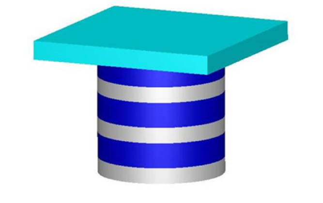
Fig. 8.1.18 Stack of disks with a square top.

This problem can be described as a single UNIT problem, describing the cylindrical portion first. In this instance, the origin has been chosen at the center bottom of the bottom disk. The bottom disk is defined by the first cylinder description, and the next disk is defined by the difference between the first and second cylinder descriptions. Since both disks have a radius of 5.0 and a -Z length of 0.0, the first cylinder containing material 1 exists from Z = 0.0 to Z = 2.0, and the second cylinder containing material 2 exists from Z = 2.0 to Z = 4.0. When all the disks have been described, a void cuboid having the same X and Y dimensions as the square plate and the same Z dimensions as the stack of disks is defined. The square plate of material 3 is then defined on top of the stack. Omission of the first cuboid description would result in the stack of disks being encased in a solid cuboid of material 3 instead of having a flat plate on top of the stack. The geometry input is shown below.

Data description 1, Example 1.

KENO V.a:

READ GEOM
CYLINDER 1  1     5.0 2.0    0.0
CYLINDER 2  1     5.0 4.0    0.0
CYLINDER 1  1     5.0 6.0    0.0
CYLINDER 2  1     5.0 8.0    0.0
CYLINDER 1  1     5.0 10.0   0.0
CYLINDER 2  1     5.0 12.0   0.0
CUBOID 0 1 10.0 -10.0 10.0 -10.0 12.0 0.0
CUBOID 3 1 10.0 -10.0 10.0 -10.0 14.5 0.0

KENO-VI:

READ GEOM
GLOBAL UNIT 1
CYLINDER   1   5.0   2.0   0.0
CYLINDER   2   5.0   4.0   2.0
CYLINDER   3   5.0   6.0   4.0
CYLINDER   4   5.0   8.0   6.0
CYLINDER   5   5.0  10.0   8.0
CYLINDER   6   5.0  12.0  10.0
CUBOID     7  10.0 -10.0  10.0 -10.0  12.0  0.0
CUBOID     8  10.0 -10.0  10.0 -10.0  14.5  0.0
MEDIA 1 1 1
MEDIA 2 1 2
MEDIA 1 1 3
MEDIA 2 1 4
MEDIA 1 1 5
MEDIA 2 1 6
MEDIA 0 1 -1 -2 -3 -4 -5 -6 7
MEDIA 3 1 -7 8
BOUNDARY  8
END GEOM

An alternative description of the same example is given below. The origin has been chosen at the center of the disk of material 1 nearest the center of the stack. This disk of material 1 is defined by the first cylinder description, and the disks of material 2 on either side of it are defined by the second cylinder description. The top and bottom disks of material 1 are defined by the third cylinder, and the top disk of material 2 is defined by the last cylinder. The square plate is defined by the two cuboids. This description is more efficient than the previous one because there are fewer surfaces to check for crossings.

Data description 2, Example 1.

KENO V.a:

READ GEOM
CYLINDER 1 1  5.0   1.0 -1.0
CYLINDER 2 1  5.0   3.0 -3.0
CYLINDER 1 1  5.0   5.0 -5.0
CYLINDER 2 1  5.0   7.0 -5.0
CUBOID   0 1 10.0 -10.0 10.0 -10.0 7.0 -5.0
CUBOID   3 1 10.0 -10.0 10.0 -10.0 9.5 -5.0

KENO-VI:

READ GEOM
GLOBAL UNIT 1
CYLINDER 10  5.0   1.0 -1.0
CYLINDER 20  5.0   3.0 -3.0
CYLINDER 30  5.0   5.0 -5.0
CYLINDER 40  5.0   7.0 -5.0
CUBOID   50 10.0 -10.0 10.0 -10.0 7.0 -5.0
CUBOID   60 10.0 -10.0 10.0 -10.0 9.5 -5.0
MEDIA 1 1 10
MEDIA 2 1 -10 20
MEDIA 1 1 -20 30
MEDIA 2 1 -30 40
MEDIA 0 1 -40 50
MEDIA 3 1 -50 60
BOUNDARY  60
END GEOM

Example 1 can also be described as an ARRAY. Define three different UNIT types. UNIT 1 will define a disk of material 1, UNIT 2 will define a disk of material 2, and UNIT 3 will define the square plate of material 3. The origin of each UNIT is defined at the center bottom of the disk or plate being described. As mentioned earlier, only UNITs with a CUBE or CUBOID as their outer boundary can be placed in a cuboidal ARRAY. The geometry input for this arrangement is shown below.

Data description 3, Example 1.

KENO V.a:

READ GEOM
UNIT 1
CYLINDER  1 1  5.0   2.0  0.0
CUBOID    0 1 10.0 -10.0 10.0 -10.0 2.0 0.0
UNIT 2
CYLINDER  2 1  5.0   2.0  0.0
CUBOID    0 1 10.0 -10.0 10.0 -10.0 2.0 0.0
UNIT 3
CUBOID    3 1 10.0 -10.0 10.0 -10.0 2.5 0.0
END GEOM
READ ARRAY  NUX=1 NUY=1 NUZ=7 FILL 1 2 1 2 1 2 3 END ARRAY

Note

The ARRAY is assumed to be the GLOBAL ARRAY because only a single ARRAY is defined.

KENO-VI:

READ GEOM
UNIT 1
CYLINDER 1  5.0   2.0  0.0
CUBOID  2 10.0 -10.0 10.0 -10.0 2.0 0.0
MEDIA 1 1 1
MEDIA 0 1 -1 2
BOUNDARY 2
UNIT 2
CYLINDER  1  5.0   2.0  0.0
CUBOID    2 10.0 -10.0 10.0 -10.0 2.0 0.0
MEDIA 2 1 1
MEDIA 0 1 2 -1
BOUNDARY 2
UNIT 3
CUBOID    1 10.0 -10.0 10.0 -10.0 2.5 0.0
MEDIA 3 1 1
BOUNDARY 1
GLOBAL UNIT 4
CUBOID 1  10 -10 10 -10 14.5 0.0
ARRAY 1 1  PLACE 1 1 1 3*0.0
BOUNDARY 1
END GEOM
READ ARRAY ARA=1 NUX=1 NUY=1 NUZ=7 FILL 1 2 1 2 1 2 3 END ARRAY

If the user prefers for the origin of each unit to be at its center, the geometry region data can be entered as shown below. The array data would be identical to that of data description 3, Example 1.

Data description 4, Example 1.

KENO V.a:

READ GEOM
UNIT 1
CYLINDER  1 1  5.0   1.0 -1.0
CUBOID    0 1 10.0 -10.0 10.0 -10.0 1.0 -1.0
UNIT 2
CYLINDER  2 1  5.0   1.0 -1.0
CUBOID    0 1 10.0 -10.0 10.0 -10.0 1.0 -1.0
UNIT 3
CUBOID  3 1 10.0 -10.0 10.0 -10.0 1.25 -1.25
END GEOM

KENO-VI:

READ GEOM
UNIT 1
CYLINDER 1  5.0   1.0 -1.0
CUBOID  2   10.0 -10.0 10.0 -10.0 1.0 -1.0
MEDIA 1 1 1
MEDIA 0 1 -1 2
BOUNDARY  2
UNIT 2
CYLINDER 1  5.0   1.0 -1.0
CUBOID  2  10.0 -10.0 10.0 -10.0 1.0 -1.0
MEDIA 2 1 1
MEDIA 0 1 -1 2
BOUNDARY  2
UNIT 3
CUBOID 1 10.0 -10.0 10.0 -10.0 1.25 -1.25
MEDIA 3 1 1
BOUNDARY  1
GLOBAL UNIT 4
CUBOID 1 10 -10 10 -10 14.5 0.0
ARRAY 1 1 PLACE 1 1 1 0.0 0.0 1.0
BOUNDARY 1
END GEOM

Be aware that each UNIT in a geometry description can have its origin defined independent of the other UNITs. It would be correct to use UNITs 1 and 3 from data descriptions 3, and UNIT 2 from data description 4. The array data would remain the same as data description 3, Example 1. The user should define the origin of each unit to be as convenient as possible for the chosen description. Care should be taken when assigning coordinates to the UNIT used to PLACE the ARRAY in its surrounding region.

Another method of describing Example 1 as a bare array is to define UNIT 1 to be a disk of material 1 topped by a disk of material 2. The origin has been chosen at the center bottom of the disk of material 1. UNIT 2 is the square plate of material 3 with the origin at the center of the UNIT. The ARRAY consists of three UNIT 1s, topped by a UNIT 2, as shown below.

Data description 5, Example 1.

KENO V.a:

READ GEOM
UNIT 1
CYLINDER  1 1  5.0   2.0  0.0
CYLINDER  2 1  5.0   4.0  0.0
CUBOID    0 1 10.0 -10.0 10.0 -10.0 4.0 0.0
UNIT 2
CUBOID    3 1 10.0 -10.0 10.0 -10.0 1.25 -1.25
END GEOM
READ ARRAY  NUX=1 NUY=1 NUZ=4 FILL 3R1 2 END ARRAY

KENO-VI:

READ GEOM
UNIT 1
CYLINDER  1  5.0   2.0  0.0
CYLINDER  2  5.0   4.0  2.0
CUBOID  3   10.0 -10.0 10.0 -10.0 4.0 0.0
MEDIA 1 1 1
MEDIA 2 1 2
MEDIA 0 1 -1 -2 3
BOUNDARY  3
UNIT 2
CUBOID  1  10.0 -10.0 10.0 -10.0 1.25 -1.25
MEDIA 3 1 1
BOUNDARY  1
GLOBAL UNIT 3
CUBOID  1 10 -10 10 -10 14.5 0.0
ARRAY 1 1 PLACE 1 1 1 3*0.0
BOUNDARY  1
END GEOM
READ ARRAY  ARA=1 NUX=1 NUY=1 NUZ=4 FILL 3R1 2 END ARRAY

Example 1 can be described as a reflected ARRAY by treating the square plate as a reflector in the positive Z direction. One means of describing this situation is to define UNITs 1 and 2 as in data description 3, Example 1. The origin of the GLOBAL UNIT is defined to be at the center of the ARRAY. The corresponding input geometry is shown below.

Data description 6, Example 1.

KENO V.a:

READ GEOM
UNIT 1
CYLINDER  1 1   5.0   2.0  0.0
CUBOID    0 1  10.0  -10.0  10.0  -10.0  2.0  0.0
UNIT 2
CYLINDER  2 1   5.0   2.0  0.0
CUBOID      0 1  10.0  -10.0  10.0  -10.0  2.0  0.0
GLOBAL UNIT 3
ARRAY        1 -10.0  -10.0  -6.0
CUBOID     3 1  10.0  -10.0  10.0  -10.0  8.5  -6.0
END GEOM
READ ARRAY  NUX=1 NUY=1 NUZ=6 FILL 1 2 1 2 1 2 END ARRAY

KENO-VI:

READ GEOM
UNIT 1
CYLINDER  1  5.0   2.0  0.0
CUBOID  2   10.0 -10.0 10.0 -10.0 2.0  0.0
MEDIA 1 1 1
MEDIA 0 1 -1 2
BOUNDARY  2
UNIT 2
CYLINDER  1  5.0   2.0  0.0
CUBOID  2  10.0 -10.0 10.0 -10.0 2.0  0.0
MEDIA 2 1 1
MEDIA 0 1 -1 2
BOUNDARY  2
GLOBAL UNIT 3
CUBOID 1  10.0 -10.0 10.0 -10.0 6.0 -6.0
CUBOID 2  10.0 -10.0 10.0 -10.0 8.5 -6.0
ARRAY 1 1 PLACE 1 1 1 0.0 0.0 -6.0
MEDIA 3 1 -1 2
BOUNDARY  2
END GEOM
READ ARRAY ARA=1 NUX=1 NUY=1 NUZ=6 FILL 1 2 1 2 1 2 END ARRAY

The user could have chosen the origin of the ARRAY boundary to be at the center bottom of the ARRAY, in which case the geometry description for the GLOBAL UNIT would be:

KENO V.a:

ARRAY       1 -10.0  -10.0  0.0
CUBOID   3 1 10.0  -10.0  10.0  -10.0  14.5  0.0

or

ARRAY    1  -10.0  -10.0 0.0
REPLICATE  3  4*0.0  2.5  0 1

The reflector region at the top of the array can be added by using a CUBOID or by using a REPLICATE description in KENO V.a. Recall that there is no REPLICATE function in KENO-VI.

A simpler method of describing Example 1 as a reflected array is to define only one unit as in data description 5, Example 1. The square plate is treated as a reflector, as in data description 6, Example 1. The input for this arrangement is given below.

Data description 7, Example 1.

KENO V.a:

READ GEOM
UNIT 1
CYLINDER  1 1   5.0   2.0  0.0
CYLINDER  2 1   5.0   4.0  0.0
CUBOID      0 1  10.0  -10.0  10.0  -10.0  4.0  0.0
GLOBAL UNIT 2
ARRAY        1  -10.0  -10.0  0.0
CUBOID     3  1  10.0  -10.0  10.0  -10.0  14.5  0.0
END GEOM
READ ARRAY NUX=1 NUY=1 NUZ=3 END ARRAY

KENO-VI:

READ GEOM
UNIT 1
CYLINDER  1   5.0   2.0  0.0
CYLINDER  2   5.0   4.0  2.0
CUBOID   3   10.0 -10.0 10.0 -10.0 4.0 0.0
MEDIA 1 1 1
MEDIA 2 1 2
MEDIA 0 1 -1 -2 3
BOUNDARY  3
GLOBAL UNIT 2
CUBOID  1  10.0 -10.0 10.0 -10.0  12.0 0.0
CUBOID  2  10.0 -10.0 10.0 -10.0 14.5 0.0
ARRAY 1 1 PLACE 1 1 1 3*0.0
MEDIA 3 1 -1 2
BOUNDARY  2
END GEOM
READ ARRAY ARA=1 NUX=1 NUY=1 NUZ=3 FILL F1  END FILL  END ARRAY

EXAMPLE 2. Assume that the stack of six disks in Example 1 is placed at the center bottom of a cylindrical container composed of material 6 whose inside diameter is 16.0 cm. The bottom and sides of the container are 0.25 cm thick, the top is open, and the total height of the container is 18.25 cm. Assume the square plate of Example 1 is centered on top of the container.

The geometry input can be described utilizing most of the data description methods associated with Example 1. One method of describing Example 2 as a single UNIT is given below.

Data description 1, Example 2.

KENO V.a:

READ GEOM
UNIT 1
CYLINDER  1 1  5.0    1.0  -1.0
CYLINDER  2 1  5.0    3.0  -3.0
CYLINDER  1 1  5.0    5.0  -5.0
CYLINDER  2 1  5.0    7.0  -5.0
CYLINDER  0 1  8.0   13.0  -5.0
CYLINDER  6 1  8.25  13.0  -5.25
CUBOID    0 1 10.0  -10.0  10.0 -10.0 13.0 -5.25
CUBOID    3 1 10.0  -10.0  10.0 -10.0 15.5 -5.25
END GEOM

KENO-VI:

READ GEOM
GLOBAL UNIT 1
CYLINDER  1  5.0    1.0  -1.0
CYLINDER  2  5.0    3.0  -3.0
CYLINDER  3  5.0    5.0  -5.0
CYLINDER  4  5.0    7.0  -5.0
CYLINDER  5  8.0   13.0  -5.0
CYLINDER  6  8.25  13.0  -5.25
CUBOID    7  10.0 -10.0  10.0 -10.0 13.0 -5.25
CUBOID    8  10.0 -10.0  10.0 -10.0 15.5 -5.25
MEDIA 1 1 1
MEDIA 2 1 -1 2
MEDIA 1 1 -2 3
MEDIA 2 1 -3 4
MEDIA 0 1 -4 5
MEDIA 6 1 -5 6
MEDIA 0 1 -6 7
MEDIA 3 1 -7 8
BOUNDARY  8
END GEOM

In the above description, the origin is defined to be at the center of the disk of material 1 nearest the center of the stack. This disk is defined by the first cylinder description. The disks of material 2 above and below it are defined by the second cylinder description. The disks of material 1 above and below them are defined by the third cylinder description. The top disk of material 2 is defined by the fourth cylinder description. The void interior of the container is defined by the fifth cylinder description. The container is defined by the last cylinder description. The first cuboid description is used to define a void whose X and Y dimensions are the same as the square plate and whose Z dimensions are the same as the container. The last cuboid description defines the square plate. Omission of the first cuboid description would result in the container being encased in a solid cuboid of material 3. Thus, both cuboids are necessary to properly define the square plate.

Example 2 can be described as a reflected ARRAY. One of the descriptions uses only one UNIT and is similar to data description 7, Example 1. This description is shown below.

Data description 2, Example 2.

KENO V.a:

READ GEOM
UNIT 1
CYLINDER  1  1  5.0    2.0   0.0
CYLINDER  2  1  5.0    4.0   0.0
CUBOID    0 1  5.0   -5.0   5.0   -5.0  4.0  0.0
GLOBAL UNIT 2
ARRAY          1  -5.0   -5.0   0.0
CYLINDER  0  1  8.0   18.0   0.0
CYLINDER  6  1  8.25  18.0  -0.25
CUBOID      0  1  10.0  -10.0  10.0  -10.0  18.0  -0.25
CUBOID      3  1  10.0  -10.0  10.0  -10.0  20.5  -0.25
END GEOM
READ ARRAY  NUX=1 NUY=1 NUZ=3 END ARRAY

KENO-VI:

READ GEOM
UNIT 1
CYLINDER  1  5.0    2.0   0.0
CYLINDER  2  5.0    4.0   2.0
CUBOID    3  5.0   -5.0   5.0   -5.0  4.0  0.0
MEDIA 1 1 1
MEDIA 2 1 2
MEDIA 0 1 -1 -2 3
BOUNDARY  3
GLOBAL UNIT 2
CUBOID   1 5.0 -5.0 5.0 -5.0 12.0 0.0
ARRAY 1 1 PLACE 1 1 1 3*0.0
CYLINDER  2  8.0   18.0   0.0
MEDIA 0 1 -1 2
CYLINDER  3  8.25  18.0  -0.25
MEDIA 6 1 -2 3
CUBOID    4 10.0  -10.0  10.0  -10.0 20.5 18.0
CUBOID    5 10.0  -10.0  10.0  -10.0 20.5 -0.25
MEDIA 3 1 4
MEDIA 0 1 -3 -4 5
BOUNDARY  5
END GEOM
READ ARRAY ARA NUX=1 NUY=1 NUZ=3 FILL F1 END FILL END ARRAY

In the above data description, the first two cylinder descriptions define a disk of material 1 with a disk of material 2 directly on top of it. A tight fitting void cuboid is placed around them so they can be stacked three high to achieve the stack of disks shown in Example 1, Fig. 8.1.18. This array comprises the array portion of the geometry region description. The origin of the array boundary, a tight fitting cube or cuboid that encompasses the array, is defined by the ARRAY description. Everything after the ARRAY record is considered part of the reflector. The first cylinder after the ARRAY record defines the void interior of the cylindrical container. The next cylinder defines the walls of the container. The second-to-last cuboid defines a void volume outside the container from its bottom to its top and having the same X and Y dimensions as the square plate. The last cuboid defines the square plate of material 3 that is sitting on top of the container.

Another method to describe Example 2 is as an array composed of units that contain both the stack and container. This description requires a minimum of four units to describe the problem. This configuration is given below in data description 3, Example 2.

Data description 3, Example 2.

KENO V.a:

READ GEOM
UNIT 1
CYLINDER  6 1  8.25   0.25   0.0
CUBOID    0 1 10.0  -10.0   10.0 -10.0 0.25  0.0
UNIT 2
CYLINDER  1 1  5.0    2.0    0.0
CYLINDER  2 1  5.0    4.0    0.0
CYLINDER  0 1  8.0    4.0    0.0
CYLINDER  6 1  8.25   4.0    0.0
CUBOID    0 1 10.0  -10.0   10.0 -10.0 4.0   0.0
UNIT 3
CYLINDER  0 1  8.0    3.0   -3.0
CYLINDER  6 1  8.25   3.0   -3.0
CUBOID    0 1 10.0  -10.0   10.0 -10.0 3.0  -3.0
CUBOID    3 1 10.0  -10.0   10.0 -10.0 5.5  -3.0
END GEOM
READ ARRAY  NUX=1 NUY=1 NUZ=5 FILL 1 3R2 3 END ARRAY

KENO-VI:

READ GEOM
UNIT 1
CYLINDER  1  8.25   0.25   0.0
CUBOID  2   10.0  -10.0   10.0 -10.0 0.25  0.0
MEDIA 6 1 1
MEDIA 0 1 2 -1
BOUNDARY  2
UNIT 2
CYLINDER  10  5.0    2.0    0.0
CYLINDER  20  5.0    4.0    0.0
CYLINDER  30  8.0    4.0    0.0
CYLINDER  40  8.25   4.0    0.0
CUBOID  50   10.0  -10.0   10.0 -10.0 4.0   0.0
MEDIA 1 1 10
MEDIA 2 1 20 -10
MEDIA 0 1 30 -20
MEDIA 6 1 40 -30
MEDIA 0 1 50 -40
BOUNDARY  50
UNIT 3
CYLINDER  1  8.0    3.0   -3.0
CYLINDER  2  8.25   3.0   -3.0
CUBOID    3 10.0  -10.0   10.0 -10.0 5.5   3.0
CUBOID    4 10.0  -10.0   10.0 -10.0 5.5  -3.0
MEDIA 0 1 1
MEDIA 6 1 2 -1
MEDIA 3 1 3
MEDIA 0 1 4 -3 -2
BOUNDARY  4
GLOBAL UNIT 4
CUBOID  1  10.0 -10.0 10.0 -10.0 20.75 0.0
ARRAY 1 1 PLACE 1 1 1 3*0.0
BOUNDARY  1
END GEOM
READ ARRAY  NUX=1 NUY=1 NUZ=5 FILL 1 3R2 3 END ARRAY

In the above description, UNIT 1 is the bottom of the cylindrical container. The void CUBOID is only as tall as the bottom of the container, and its X and Y dimensions are the same as the square plate on top of the container. If all the UNITs in the ARRAY use these same dimensions in the X and Y directions, the requirement that adjacent faces of units in contact with each other must be the same size and shape is satisfied. This ARRAY is stacked in the Z direction, so all UNITs must have the same overall dimensions in the X direction and in the Y direction. UNIT 2 will be used in the ARRAY three times to create the stack of disks. It contains a disk of material 1 topped by a disk of material 2. The portion of the container that contains the disks and the cuboid that defines the outer boundaries of the unit are included in UNIT 2. UNIT 3 describes the empty top portion of the container and the square plate on top of it. The Z dimensions of UNIT 3 were determined by subtracting three times the total Z dimension of UNIT 2 from the inside height of the container [18.0 - (3 \(\times\) 4.0) = 6.0]. This can also be determined from the overall height of the container by subtracting off the bottom thickness of the container and three times the height of UNIT 2 [18.25 - 0.25 - (3 \(\times\) 4.0) = 6.0]. The origin of UNIT 3 is located at the center of this distance. For the KENO-VI input, a GLOBAL UNIT is also provided, UNIT 4, containing the ARRAY built with UNITs 1, 2, 3.

EXAMPLE 3. Refer to Example 1, Fig. 8.1.18, and imagine a HOLE 1.5 cm in diameter is drilled along the centerline of the stack through the disks and the square plate. In KENO V.a this HOLE would eliminate the possibility of describing the system as a single unit because the HOLE in the center of the alternating materials of the stack cannot be described in a manner that allows each successive geometry region to encompass the regions interior to it. Therefore, it must be described as an ARRAY. The square plate on the top of the disks is defined as a UNIT in the ARRAY. In the geometry description given below, the square plate is defined in UNIT 3. KENO-VI can easily describe this configuration as a single UNIT.

Data description 1, Example 3.

KENO V.a:

READ GEOM
UNIT 1
CYLINDER  0 1  0.75   2.0  0.0
CYLINDER  1 1  5.0    2.0  0.0
CUBOID    0 1 10.0  -10.0 10.0 -10.0 2.0 0.0
UNIT 2
CYLINDER  0 1  0.75   2.0  0.0
CYLINDER  2 1  5.0    2.0  0.0
CUBOID    0 1 10.0  -10.0 10.0 -10.0 2.0 0.0
UNIT 3
CYLINDER  0 1  0.75   2.5  0.0
CUBOID    3 1 10.0  -10.0 10.0 -10.0 2.5 0.0
END GEOM
READ ARRAY  NUX=1 NUY=1 NUZ=7 FILL 1 2 2Q2 3 END FILL END ARRAY

KENO-VI:

READ GEOM
GLOBAL UNIT 1
CYLINDER  1  0.75     7.0  -5.0
CYLINDER  2  5.0      1.0  -1.0
CYLINDER  3 5.0      3.0  -3.0
CYLINDER  4 5.0      5.0  -5.0
CYLINDER  5 5.0      7.0  -5.0
CYLINDER  6 8.0    13.0  -5.0
CYLINDER  7 8.25  13.0  -5.25
CUBOID  8  10.0  -10.0  10.0 -10.0 15.5  13.0
CUBOID   9 10.0  -10.0  10.0 -10.0 15.5 -5.25
MEDIA 0 1  1
MEDIA 1 1 -1  2
MEDIA 2 1 -1 -2  3
MEDIA 1 1 -1 -3  4
MEDIA 2 1 -1 -4  5
MEDIA 0 1 -5  6
MEDIA 6 1 -6  7
MEDIA 3 1  8
MEDIA 0 1 -7 -8  9
BOUNDARY   9
END GEOM

In data description 1, Example 3 above, KENO V.a input, UNIT 1 describes a disk of material 1 with a HOLE through its centerline. The first CYLINDER defines the HOLE, the second defines the rest of the disk, and the CUBOID defines the size of the UNIT to be consistent with the square plate so they can be stacked together in an ARRAY. UNIT 2 describes a disk of material 2 in similar fashion. UNIT 3 describes the square plate of material 3 with a HOLE through its center. The CYLINDER defines the HOLE and the CUBOID defines the square plate. These three UNITs are stacked in the Z direction to achieve the composite system. This is represented by FILL122Q23. The 2Q2 repeats the two entries preceding the 2Q2 twice. Alternatively, this can be achieved by entering FILL 1 2 1 2 1 2 3 END FILL. The same ARRAY can also be achieved using the LOOP option. An example of the data for this option is:

LOOP 1 6R1 1 5 2 2 6R1 2 6 2 3 6R1 7 7 1 END LOOP.

UNIT 1 is placed at the X = 1, Y = 1, and Z = 1,3,5 positions of the ARRAY by entering 1 6R1 1 5 2. UNIT 2 is positioned at the X = 1, Y = 1 and Z = 2,4,6 positions in the ARRAY by entering 2 6R1 2 6 2. UNIT 3 is placed at the X = 1, Y = 1, Z = 7 position of the ARRAY by entering 3 6R1 7 7 1. See Sect. 8.1.3.5 for additional information regarding ARRAY specifications.

For the KENO-VI input, UNIT 1 contains the entire problem description. The first CYLINDER describes the 1.5 cm diameter hole through the stack. The next four CYLINDERs define the stack. The sixth and seventh CYLINDERs describe the void and container. The two CUBOIDs describe the top plate and surrounding global region of void. The MEDIA cards are used to place the materials in the appropriate regions.

EXAMPLE 4. Assume two large cylinders that are 2.5 cm in radius and 5 cm long are connected by a smaller cylinder that is 0.5 cm in radius and 10 cm long, as shown in Fig. 8.1.19. All three cylinders are composed of material 1. By starting the geometry description in the small cylinder, this system can be described as a single unit.

Fig. 8.1.19 Two large cylinders joined axially by a small cylinder.

Data description 1, Example 4.

KENO-VI:

READ GEOM
GLOBAL UNIT 1
XCYLINDER  1  0.5  5.0  -5.0
XCYLINDER  2  2.5  5.0  -5.0
XCYLINDER  3  2.5 10.0 -10.0
MEDIA 1 1 1
MEDIA 0 1 2 -1
MEDIA 1 1 3 -2
BOUNDARY  3
END GEOM

KENO V.a:

READ GEOM
CYLINDER  1 1 0.5  5.0  -5.0
CYLINDER  0 1 2.5  5.0  -5.0
CYLINDER  1 1 2.5 10.0 -10.0
END GEOM

The origin is at the center of the small cylinder, which is described by the first cylinder description. The second cylinder description defines a void cylinder surrounding the small cylinder. Its radius is the same as the large cylinders, and its height (length) coincides with that of the small cylinder. The last cylinder description defines the large cylinders on either end of the small cylinder. In KENO V.a, because this problem does not specify otherwise, the length of the CYLINDERs is assumed to coincide with the Z axis. In KENO-VI, because the problem was created using XCYLINDERs, the long axes of the CYLINDERs coincide with the X axis.

EXAMPLE 5. Assume two large cylinders with a center-to-center spacing of 15 cm, each having a radius of 2.5 cm and length of 5 cm, are connected radially by a small cylinder having a radius of 1.5 cm, as shown in Fig. 8.1.20.

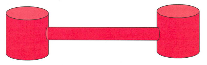
Fig. 8.1.20 Two large cylinders radially connected by a small cylinder.

This system cannot be described rigorously in KENO V.a geometry because the intersection of the cylinders cannot be described. However, it can be approximated two ways, as shown in Fig. 8.1.21. The top approximation is described in data description 1, Example 5. The bottom approximation is described in data description 2, Example 5, and data description 3, Example 5. These may be poor approximations for criticality safety calculations.

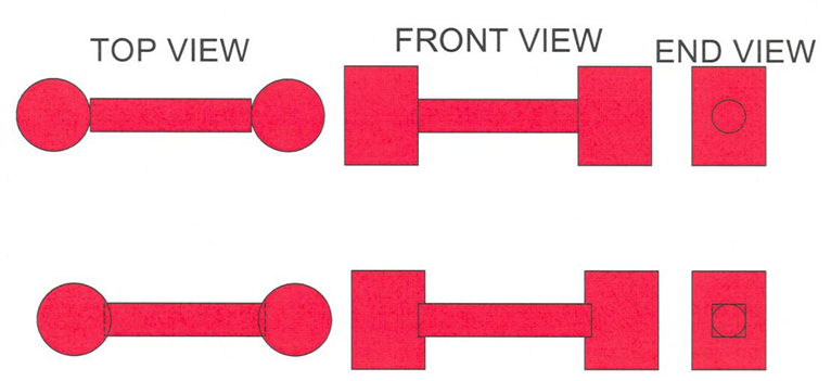
Fig. 8.1.21 KENO V.a approximations of cylindrical intersections.

Data description 1, Example 5.

KENO V.a:

READ GEOM
UNIT 1
CYLINDER  1 1 2.5 2.5 -2.5
CUBE      0 1 2.5 -2.5
UNIT 2
XCYLINDER 1 1 1.5 5.0 -5.0
CUBOID    0 1 5.0 -5.0 2.5 -2.5 2.5 -2.5
END GEOM
READ ARRAY NUX=3 NUY=1 NUZ=1 FILL 1 2 1 END ARRAY

UNIT 1 defines a large CYLINDER, and UNIT 2 describes the small CYLINDER. In both UNITs the origin is at the center of the CYLINDER. The large CYLINDERs have their centerlines along the Z axis and the small CYLINDER has its length along the X axis.

Data description 2, Example 5.

KENO V.a:

READ GEOMETRY
UNIT 1
CYLINDER 1 1 2.5 1.0 0.0
CUBOID 0 1 4P2.5 1.0 0.0
UNIT 2
ZHEMICYL-X 1 1 2.5 2P1.5 CHORD 2.0
CUBOID 0 1 2.0 3P-2.5 2P1.5
UNIT 3
ZHEMICYL+X 1 1 2.5 2P1.5 CHORD 2.0
CUBOID 0 1 2.5 -2.0 2P2.5 2P1.5
UNIT 4
XCYLINDER 1 1 1.5 2P5.5
CUBOID 0 1 2P5.5 2P2.5 2P1.5
UNIT 5
CUBOID 0 1 2P5.0 2P2.5 1.0 0.0
UNIT 6
ARRAY 1 3*0.0
UNIT 7
ARRAY 2 3*0.0
END GEOMETRY
READ ARRAY ARA=1 NUX=3 NUY=1 NUZ=1 FILL 1 5 1 END FILL
ARA=2 NUX=3 NUY=1 NUZ=1 FILL 2 4 3 END FILL
ARA=3 NUX=1 NUY=1 NUZ=3 FILL 6 7 6 END FILL
END ARRAY

The above geometry description uses ARRAYs of ARRAYs (see Sect. 8.1.4.6.3) to describe the bottom approximation of Fig. 8.1.21. UNIT 1 defines a large CYLINDER that has a radius of 2.5 cm and a height of 10 cm inside a close-fitting CUBOID. This is used in both large CYLINDERs as the portion of the large CYLINDER that exists above and below the region where the small CYLINDER joins it. UNIT 5 is the spacing between the tops of the two large CYLINDERs and the spacing between the bottoms of the two large CYLINDERs. ARRAY 1 thus defines the bottom of the system: two short CYLINDERs (UNIT 1s) separated by 10 cm (UNIT 5 is the separation). UNIT 6 contains ARRAY 1.

UNIT 2 is the left hemicylinder that adjoins the horizontal CYLINDER, and UNIT 3 is the right hemicylinder that adjoins the horizontal CYLINDER. UNIT 4 defines the horizontal CYLINDER. ARRAY 2 contains UNITs 2, 4, and 3 from left to right. This defines the central portion of the system where the horizontal CYLINDER adjoins the two hemicylinders. These hemicylinders are larger than half CYLINDERs. UNIT 7 contains ARRAY 2. The entire system is achieved by stacking a UNIT 6 above and below the UNIT 7 as defined in ARRAY 3, the GLOBAL ARRAY.

Data description 3, Example 5.

KENO V.a:

READ GEOMETRY
UNIT 1
CYLINDER 1 1 2.5 1.0 0.0
UNIT 2
CYLINDER 1 1 2.5 1.0 0.0
CUBOID 0 1 17.5 -2.5 2P2.5 1.0 0.0
HOLE 1 15.0 0.0 0.0
UNIT 3
ZHEMICYL-X 1 1 2.5 2P1.5 CHORD 2.0
UNIT 4
ZHEMICYL+X 1 1 2.5 2P1.5 CHORD 2.0
UNIT 5
XCYLINDER  1 1 1.5 2P5.5
CUBOID 0 1  2P10.0 2P2.5 2P1.5
HOLE 3 -7.5 2*0.0
HOLE 4 7.5 2*0.0
END GEOMETRY
READ ARRAY
ARA=1 NUX=1 NUY=1 NUZ=3 FILL 2 5 2 END FILL
END ARRAY

The above geometry description uses HOLEs (see Sect. 8.1.4.6.1) to describe the bottom approximation of Fig. 8.1.21. UNIT 1 defines a large CYLINDER with a radius of 2.5 cm and a height of 1.0 cm. UNIT 2 defines the same CYLINDER within a CUBOID that extends from X = -2.5 to X = 17.5, from Y = -2.5 to Y = 2.5, and Z = 0.0 to Z = 1.0. The origin of the CYLINDER is at (0.0,0.0,0.0). Thus UNIT 2 describes the top and bottom of the CYLINDER on the left. UNIT 1 is positioned within this CUBOID as a HOLE with its origin at (15.0,0.0,0.0) to describe the top and bottom of the CYLINDER on the right. UNIT 3 is the left hemicylinder that adjoins the horizontal CYLINDER, and UNIT 4 is the right hemicylinder that adjoins the horizontal CYLINDER. UNIT 5 defines the horizontal CYLINDER with its origin at the center within a CUBOID that extends from X = -10.0 to X = +10.0, Y = -2.5 to Y = 2.5, and Z = -1.5 to Z = 1.5. UNIT 3 is positioned to the left of the horizontal CYLINDER, and UNIT 4 is positioned to the right of the horizontal CYLINDER by using HOLEs. The entire system is achieved by stacking a UNIT 2 above and below UNIT 5 as shown in the ARRAY data.

This same geometry description can be used with UNIT 2 redefined, having its origin defined so that it extends from X = -10 to X = 10, Y = -2.5 to Y = 2.5, and Z = 0.0 to Z = 1. In this instance, the geometry data would be identical except for UNIT 2. This alternative description of UNIT 2 is

KENO V.a:

UNIT 2
CYLINDER 1 1 2.5 1.0 0.0 ORIGIN -7.5 0.0
CUBOID 0 1 2P10.0 2P2.5 1.0 0.0
HOLE 1 7.5 0.0 0.0

This system can be easily described in KENO-VI geometry because intersections are allowed. The small CYLINDER is rotated in data description 1, Example 5.

Data description 1, Example 5.

KENO-VI:

READ GEOM
GLOBAL UNIT 1
CYLINDER   1  2.5  2.5 -2.5
CYLINDER   2  2.5  2.5 -2.5 ORIGIN Y=15.0
YCYLINDER  3  1.5 15.0  0.0
CUBOID     4  5.0 -5.0 17.5 -2.5 2.5 -2.5
MEDIA 1 1 1
MEDIA 1 1 2
MEDIA 1 1 3 -1 -2
MEDIA 0 1 4 -3 -2 -1
BOUNDARY  4
END GEOM

The first and second CYLINDERs define the two large CYLINDERs, and the third CYLINDER describes the small connecting CYLINDER. The two large CYLINDERs are oriented along the Z axis. The second large cylinder is translated so its origin is at position (0.0, 15.0, 0.0). The small CYLINDER is oriented along the Y axis. Region 1 consists of the material in the first large CYLINDER. Region 2 consists of the material in the second large CYLINDER. Region 3 consists of the material in the small CYLINDER but not in either of the large CYLINDERs. Region 4 is the BOUNDARY region.

EXAMPLE 6. Assume 2 small cylinders 1.0 cm in radius and 10 cm long are connected by a large cylinder 2.5 cm in radius and 5 cm long as shown in Fig. 8.1.22.

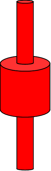
Fig. 8.1.22 Two small cylinders joined axially by a large cylinder.

This problem is very similar to Example 4. It can be described as a single UNIT in KENO-VI, but not in KENO V.a where it must be described as an array. In KENO V.a, UNIT 1 defines the large cylinder, and UNIT 2 defines the small cylinder. The origin of each UNIT is at its center. The composite system consists of two UNIT 2s and one UNIT 1 as shown below. In KENO-VI, CYLINDER 1 defines the long thin cylinder, and CYLINDER 2 defines the short thick cylinder. The origin of each cylinder is at its center. In both KENO V.a and KENO-VI, the centerline of the cylinders lies along the Z axis.

Data description 1, Example 6.

KENO V.a:

READ GEOM
UNIT 1
CYLINDER  1 1 2.5 2.5 -2.5
CUBE      0 1 2.5 -2.5
UNIT 2
CYLINDER  1 1 1.0 5.0 -5.0
CUBOID    0 1 2.5 -2.5 2.5 -2.5 5.0 -5.0
END GEOM
READ ARRAY NUX=1 NUY=1 NUZ=3 FILL 2 1 2 END ARRAY

KENO-VI:

READ GEOM
GLOBAL UNIT 1
CYLINDER  1  1.0 12.5  -12.5
CYLINDER  2  2.5  2.5   -2.5
CUBOID    3  4P2.5 12.5 -12.5
MEDIA 1 1 1
MEDIA 1 1 2 -1
MEDIA 0 1 3 -2 -1
BOUNDARY  3
END GEOM

EXAMPLE 7. Assume an 11 \(\times\) 5 \(\times\) 3 square-pitched array of spheres of material 1, radius 3.75 cm, with a center-to-center spacing of 10 cm in the X, Y, and Z directions. The data for this system are given below.

Data description 1, Example 7.

KENO V.a:

READ GEOM
SPHERE 1 1 3.75
CUBE   0 1 5.0 -5.0
END GEOM
READ ARRAY NUX=11  NUY=5 NUZ=3 END ARRAY

KENO-VI:

READ GEOM
UNIT 1
SPHERE  1  3.75
CUBOID  2  6P5.0
MEDIA 1 1 1
MEDIA 0 1 2 -1
BOUNDARY  2
GLOBAL UNIT 2
CUBOID 10 55.0 -55.0 25.0 -25.0 15.0 -15.0
ARRAY 1 10 PLACE 6 3 2 3*0.0
BOUNDARY  10
END GEOM
READ ARRAY NUX=11  NUY=5 NUZ=3 FILL F1 END FILL END ARRAY

EXAMPLE 8. Assume an 11 \(\times\) 5 \(\times\) 3 rectangular-pitched array of spheres of material 1, whose radius is 3.75 cm and whose center-to-center spacing is 10 cm in the X direction, 15 cm in the Y direction, and 20 cm in the Z direction. The input for this geometry is given below.

Data description 1, Example 8.

KENO V.a:

READ GEOM
SPHERE  1 1 3.75
CUBOID  0 1 5.0  -5.0 7.5 -7.5 10.0 -10.0
END GEOM
READ ARRAY  NUX=11 NUY=5 NUZ=3 END ARRAY

KENO-VI:

READ GEOM
UNIT 1
SPHERE  1 3.75
CUBOID  2  5.0  -5.0 7.5 -7.5 10.0 -10.0
MEDIA 1 1 1
MEDIA 0 1 2 -1
BOUNDARY  2
GLOBAL UNIT 2
CUBOID  1  55.0 -55.0 37.5 -37.5 30.0 -30.0
ARRAY 1 1 PLACE 6 3 2 3*0.0
BOUNDARY  1
END GEOM
READ ARRAY  NUX=11 NUY=5 NUZ=3 FILL F1 END FILL END ARRAY

EXAMPLE 9. Assume an 11 \(\times\) 5 \(\times\) 3 square-pitched array of spheres of material 1 with a 3.75 cm radius and 10 cm center-to-center spacing in the X, Y, and Z directions. This array is reflected by 30 cm of material 2 (water) on all faces, and weighted tracking (biasing) is to be used in the water reflector. The array spacing defines the perpendicular distance from the outer layer of spheres to the reflector to be 5 cm in the X, Y, and Z directions. The geometry input for this system is given below.

Data description 1, Example 9.

KENO V.a:

READ GEOM
UNIT 1
SPHERE     1  1   3.75
CUBE         0  1   5.0   -5.0
GLOBAL UNIT 2
ARRAY               1  -55.0  -25.0  -15.0
REFLECTOR    2  2  6*3.0  10
END GEOM
READ ARRAY  NUX=11 NUY=5 NUZ=3 END ARRAY
READ BIAS ID=500 2 11 END BIAS

KENO-VI:

READ GEOM
UNIT 1
SPHERE  1  3.75
CUBOID  2 6P5.0
MEDIA 1 1 1
MEDIA 0 1 2 -1
BOUNDARY  2
GLOBAL UNIT 2
CUBOID  1  55.0  -55.0  25.0  -25.0  15.0  -15.0
CUBOID  2  58.0  -58.0  28.0  -28.0  18.0  -18.0
CUBOID  3  61.0  -61.0  31.0  -31.0  21.0  -21.0
CUBOID  4  64.0  -64.0  34.0  -34.0  24.0  -24.0
CUBOID  5  67.0  -67.0  37.0  -37.0  27.0  -27.0
CUBOID  6  70.0  -70.0  40.0  -40.0  30.0  -30.0
CUBOID  7  73.0  -73.0  43.0  -43.0  33.0  -33.0
CUBOID  8  76.0  -76.0  46.0  -46.0  36.0  -36.0
CUBOID  9  79.0  -79.0  49.0  -49.0  39.0  -39.0
CUBOID 10  82.0  -82.0  52.0  -52.0  42.0  -42.0
CUBOID 11  85.0  -85.0  55.0  -55.0  45.0  -45.0
ARRAY 1 1 PLACE 6 3 2 3*0.0
MEDIA 2 2 2 -1
MEDIA 2 3 3 -2
MEDIA 2 4 4 -3
MEDIA 2 5 5 -4
MEDIA 2 6 6 -5
MEDIA 2 7 7 -6
MEDIA 2 8 8 -7
MEDIA 2 9 9 -8
MEDIA 2 10 10 -9
MEDIA 2 11 11 -10
BOUNDARY  11
END GEOM
READ ARRAY  NUX=11 NUY=5 NUZ=3 FILL F1 END FILL  END ARRAY
READ BIAS ID=500 2 11 END BIAS

In the KENO V.a input, the ARRAY boundary defines the origin of the REFLECTOR to be at the center of the ARRAY. The 6*3.0 in the REFLECTOR description repeats the 3.0 six times. The REFLECTOR record is used to generate ten REFLECTOR regions, each of which is 3.0 cm thick, on all six faces of the ARRAY.

In the KENO-VI input, the basic UNIT used to construct the ARRAY is defined in UNIT 1. The ARRAY is positioned in UNIT 2 (the GLOBAL UNIT) using the ARRAY card and the PLACE option. The ARRAY is then surrounded by ten REFLECTOR regions, each 3.0 cm thick, on all sides.

The first bias ID is 2, so the last bias ID will be 11 if 10 regions are created. The biasing data block is necessary to apply the desired weighting or biasing function to the reflector. The biasing material ID is obtained from Table 8.1.25. IDs, group structure and incremental thickness for weighting data available on the KENO  weighting library. If the biasing data block is omitted from the problem description, the 10 reflector regions will not have a biasing function applied to them, and the default value of the average weight will be used. This may cause the problem to execute more slowly, and therefore require the use of more computer time.

EXAMPLE 10. Assume the reflector in Example 9 is present only on both X faces, both Y faces, and the negative Z face. The reflector is only 15.24 cm thick on these faces. The top of the array (positive Z face) is unreflected.

Data description 1, Example 10.

KENO V.a:

READ GEOM
UNIT 1
SPHERE    1  1   3.75
CUBE        0  1   5.0   -5.0
GLOBAL UNIT 2
ARRAY             1  -55.0   -25.0  -15.0
REFLECTOR  2  2  4*3.0    0.0   3.0  5
REFLECTOR  2 7  4*0.24   0.0  0.24  1
READ ARRAY NUX=11 NUY=5 NUZ=3 END ARRAY
READ BIAS ID=500 2 7 END BIAS

KENO-VI:

READ GEOM
UNIT 1
SPHERE  1 3.75
CUBOID  2 6P5.0
MEDIA 1 1 1
MEDIA 0 1 2 -1
BOUNDARY  2
GLOBAL UNIT 2
CUBOID  1  55.0  -55.0  25.0  -25.0  15.0  -15.0
CUBOID  2  58.0  -58.0  28.0  -28.0  15.0  -18.0
CUBOID  3  61.0  -61.0  31.0  -31.0  15.0  -21.0
CUBOID  4  64.0  -64.0  34.0  -34.0  15.0  -24.0
CUBOID  5  67.0  -67.0  37.0  -37.0  15.0  -27.0
CUBOID  6  70.24 -70.24 40.24 -40.24 15.0  -30.24
ARRAY 1 1 PLACE 6 3 2 3*0.0
MEDIA 2 2 2 -1
MEDIA 2 3 3 -2
MEDIA 2 4 4 -3
MEDIA 2 5 5 -4
MEDIA 2 6 6 -5
BOUNDARY  6
END GEOM
READ ARRAY  NUX=11 NUY=5 NUZ=3 FILL F1 END FILL  END ARRAY
READ BIAS ID=500 2 6 END BIAS

In the KENO V.a input, the first REFLECTOR description generates five regions around the ARRAY, each region being 3.0 cm thick in the +X, -X, +Y, -Y, and -Z directions, and of zero thickness in the +Z direction. This defines a total thickness of 15 cm of reflector material on the appropriate faces. The second REFLECTOR description generates the last 0.24 cm of material 2 on those faces. Thus, the total reflector thickness is 15.24 cm on each face of the array, except the top which has no reflector. Five reflector regions were generated by the first REFLECTOR description, and one was generated by the second REFLECTOR description; so, six biasing regions must be defined in the biasing data. Thus, the beginning bias ID is 2, and the ending bias ID is 7.

In the KENO-VI input, the first CUBOID in Unit 2 represents the boundary for the ARRAY. The next four CUBOIDs represent the first four regions around the ARRAY, each region being 3.0 cm thick in the +X, X, +Y, -Y, and -Z directions, and of zero thickness in the +Z direction. A total thickness of 12 cm of reflector material is on the appropriate faces. The last CUBOID represents the last 3.24 cm of material 2 on those faces. Thus, the total reflector thickness is 15.24 cm on each face of the array, except the top which has no reflector. The beginning bias ID is 2, and the ending bias ID is 6. The last region could either be larger or smaller than the recommended thickness to complete the reflector.

The biasing material ID and thickness per region are obtained from Table 8.1.25. The thickness per region should be very nearly the thickness per region from the table to avoid over biasing in the reflector. Partial increments at the outer region of a reflector are exempt from this recommendation. If a biasing function is not to be applied to a region generated by the REFLECTOR record, the thickness per region can be any desired thickness and the biasing data block is omitted.

EXAMPLE 11. Assume the array of Example 7 has the central unit of the array replaced by a cylinder of material 4, 5 cm in radius and 10 cm tall. Assume a 20 cm thick spherical reflector of material 3 (concrete) is positioned so its inner radius is 65 cm from the center of the array. The minimum inner radius of a spherical reflector for this array is 62.25 cm (\(\sqrt{55^{2} + 25^{2} + 15^{2} }\)). If the inner radius is smaller than this, the problem cannot be described using KENO V.a geometry.

Data description 1, Example 11.

KENO V.a:

READ GEOM
UNIT 1
SPHERE  1  1  3.75
CUBE  0  1  5.0  -5.0
UNIT 2
CYLINDER  4  1  5.0  5.0  -5.0
CUBE  0  1  5.0  -5.0
GLOBAL UNIT 2
ARRAY     1 -55.0  -25.0  -15.0
SPHERE  0  1  65.0
REPLICATE  3  2  5.0  4
END GEOM
READ ARRAY
   NUX=11 NUY=5 NUZ=3
   LOOP 1  1  11  1  1 5 1  1 3 1  2  6 6 1  3 3 1  2 2 1  END LOOP
END ARRAY
READ BIAS ID=301 2 5 END BIAS

KENO-VI:

READ GEOM
UNIT 1
SPHERE  1 3.75
CUBOID   2 6P5.0
MEDIA 1 1 1
MEDIA 0 1 2 -1
BOUNDARY  2
UNIT 2
CYLINDER 1 5.0 5.0 -5.0
CUBOID  2  6P5.0
MEDIA 4 1 1
MEDIA 0 1 2 -1
BOUNDARY  2
GLOBAL UNIT 3
CUBOID 1  55.0 -55.0 25.0 -25.0 15.0 -15.0
SPHERE 2 65.0
SPHERE 3 70.0
SPHERE 4 75.0
SPHERE 5 80.0
SPHERE 6 85.0
ARRAY 1 1 PLACE 6 3 2 3*0.0
MEDIA 0 1 2 -1
MEDIA 3 2 3 -2
MEDIA 3 3 4 -3
MEDIA 3 4 5 -4
MEDIA 3 5 6 -5
BOUNDARY  6
END GEOM
READ ARRAY
NUX=11 NUY=5 NUZ=3
LOOP 1  1  11  1  1 5 1  1 3 1 2  6 6 1  3 3 1  2 2 1 END LOOP
END ARRAY
READ BIAS ID=301 2 5 END BIAS

UNIT 1 describes the SPHERE and spacing used in the ARRAY. UNIT 2 defines the CYLINDER located at the center of the ARRAY. In KENO V.a, the ARRAY record defines the origin of the reflector to be at the center of the ARRAY, while in KENO-VI it defines the origin of the ARRAY to be at the center of the GLOBAL UNIT. The first SPHERE in the GLOBAL UNIT defines the inner radius of the reflector. The next four SPHERE and four MEDIA records of the KENO-VI input and the REPLICATE record of the KENO V.a input will generate four spherical regions of material 3, each 5.0 cm thick. The data for the BIAS block is generated in a similar manner to previous examples, except that concrete (ID=301) is used. The recommended reflector thickness is 5 cm; this thickness is incorporated explicitly in the KENO-VI model and with 4 repetitions of the 5 cm thick reflector via REPLICATE in the KENO V.a model. The first 10 entries following the word LOOP fills the 11 \(\times\) 5 \(\times\) 3 ARRAY with UNITs 1. The next 10 entries position UNIT 2 at the center of the ARRAY (X = 6, Y = 3, and Z = 2), replacing the UNIT 1 that had been placed there by the first 10 entries.

EXAMPLE 12. Assume a data profile such as fission densities is desired in a cylinder at 0.5 cm intervals in the radial direction and 1.5 cm intervals axially. The cylinder is composed of material 1 and has a radius of 5 cm and a height of 15 cm. The REPLICATE or REFLECTOR description can be used to generate these regions in KENO V.a. A biasing data block is not entered because default biasing is desired throughout the cylinder.

Data description 1, Example 12.

KENO V.a:

READ GEOM
CYLINDER  1 1 0.5 1.5 0
REFLECTOR 1 1 0.5 1.5 0 9
END GEOM

KENO-VI:

READ GEOM
GLOBAL UNIT 1
CYLINDER 1 0.5 1.5 0
CYLINDER 2 1.0 3.0 0
CYLINDER 3 1.5 4.5 0
CYLINDER 4 2.0 6.0 0
CYLINDER 5 2.5 7.5 0
CYLINDER 6 3.0 9.0 0
CYLINDER 7 3.5 10.5 0
CYLINDER 8 4.0 12.0 0
CYLINDER 9 4.5 13.5 0
CYLINDER 10 5.0 15.0 0
MEDIA 1 1 1
MEDIA 1 1 2 -1
MEDIA 1 1 3 -2
MEDIA 1 1 4 -3
MEDIA 1 1 5 -4
MEDIA 1 1 6 -5
MEDIA 1 1 7 -6
MEDIA 1 1 8 -7
MEDIA 1 1 9 -8
MEDIA 1 1 10 -9
BOUNDARY  10
END GEOM

EXAMPLE 13. (KENO-VI due to pipe junctions) Assume a cross composed of two Plexiglas cylinders (material 3) having an inner diameter of 13.335 cm and an outer diameter of 16.19 cm. The bottom and side legs of the cross are closed by a 3.17 cm thick piece of Plexiglas. From the center of the intersection, the bottom and side legs are 91.44 cm long and the top leg is 121.92 cm long. The cross is filled with a UO₂F₂ solution (material 1) to a height of 28.93 cm above the center of the cylinder intersection. The cross is then surrounded by a water reflector (material 2) that extends from the center of the intersection: 111.74 cm in the \(\pm\)X directions, 20.64 cm in the \(\pm\)Y directions, 29.03 cm in the +Z direction, and -118.428 cm in the -Z direction. A schematic of the assembly is shown in Fig. 8.1.23.

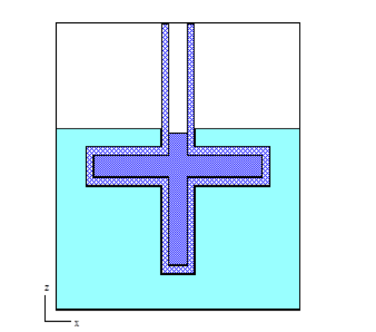
Fig. 8.1.23 Plexiglas UO₂F₂-filled cross.

Data description of Example 13 (KENO-VI only).

READ GEOMETRY
GLOBAL UNIT 1
CYLINDER   10 13.335  28.93 -88.27
CYLINDER   20 13.335 121.92 -88.27
CYLINDER   30 16.19  121.92 -91.44
YCYLINDER  40 13.335  88.27 -88.27
YCYLINDER  50 16.19 91.44 -91.44
CUBOID     60 2P111.74 2P20.64  29.03 -118.428
CUBOID     70 2P111.74 2P20.64 121.92 -118.428
MEDIA 1 1 10
MEDIA 0 1 20 -10
MEDIA 3 1 30 -20 -40
MEDIA 1 1 40 -10
MEDIA 3 1 50 -40 -30
MEDIA 2 1 60 -30 -50
MEDIA 0 1 70 -30 -60
BOUNDARY  70
END GEOMETRY

EXAMPLE 14. (KENO-VI only because of rotation) Assume a Y-shaped aluminum cylinder (material 2) with a 13.95 cm inner radius and a 0.16 cm wall thickness is filled with a UO₂F₂ solution (material 1). From the center where the Y intersects the cylinder, the bottom leg is 76.7 cm long, the top leg is 135.4 cm long, and the Y leg is 126.04 cm long, canted at a 29.26-degree angle. The bottom of the bottom leg and the top of the Y leg are sealed with 1.3 cm caps. The Y cylinder is filled to a height of 52.8 cm above the center where the Y leg intersects the vertical cylinder. The cylinder is surrounded by a water reflector (material 3) that extends out 37.0 cm in the \(\pm\)pm`Y direction, and 135.4 and -99.6 in the \(\pm\).

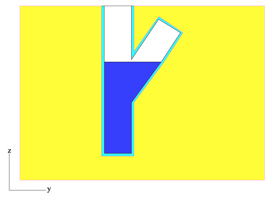
Fig. 8.1.24 Y-shaped UO₂F₂-filled aluminum cylinder.

Data description of Example 14 (KENO-VI only).

READ GEOMETRY
GLOBAL UNIT 1
COM='30 DEG Y CYLINDER'
CYLINDER 10 13.95 135.4 -75.4
CYLINDER 20 14.11 135.4 -76.7
CYLINDER 30 13.95 124.74  0.0  ROTATE A2=-29.26
CYLINDER 40 14.11 126.04  0.0 ROTATE A2=-29.26
CUBOID   50 2P37.0 100.0 -37.0 52.8 -75.4
CUBOID   60 2P37.0 100.0 -37.0 135.4 -99.6
MEDIA 1 1 10 50
MEDIA 2 1 20 -10 -30
MEDIA 1 1 30  50 -10
MEDIA 2 1 40 -30 -20
MEDIA 0 1 10 -50
MEDIA 0 1 30 -50 -10
MEDIA 3 1 60 -20 -40
BOUNDARY  60
END GEOMETRY

8.1.4.6.1. Use of holes in the geometry

Sect. 8.1.4.6 tells how each KENO V.a geometry region in a UNIT must completely enclose all previously described regions in that UNIT and how KENO-VI geometry allows regions in a UNIT to intersect, thus eliminating the need for HOLEs. HOLEs can be used to circumvent the complete enclosure restriction in KENO V.a to some degree. In KENO-VI, they can be useful in simplifying the input of a problem and decreasing the total CPU time needed for a problem. A HOLE is a means of placing an entire UNIT within a geometry region. A separate HOLE description is required for every location in a geometry region where a UNIT is to be placed. The information contained in a HOLE description is (1) the keyword HOLE, (2) the UNIT number of the UNIT to be placed, and (3) any modification data needed to correctly position and rotate (in KENO-VI) the specified UNIT within the containing UNIT. In KENO V.a, a HOLE is placed inside the geometry region that precedes it. This excludes HOLEs … (i.e., if a CUBE geometry region is followed by four HOLE descriptions, all four HOLEs are located within the CUBE). In KENO V.a, HOLEs are subject to the restriction that they cannot intersect any other geometry region. HOLEs can be nested to any depth (see Sect. 8.1.4.6.2). It is not advisable to use HOLEs tangent to other HOLEs or geometry, because round-off error may cause them to overlap. It is not uncommon for a problem that runs on one type of computer to fail on another type using the same data. Therefore, it is recommended that tangency and boundaries shared with HOLEs be avoided. This may be accomplished by separating the otherwise collocated or tangent surfaces by a very small (i.e., 10^-6 cm) distance.

In KENO V.a, tracking in regions that contain holes is less efficient than tracking in regions that do not contain holes. Therefore, holes should be used only when the system cannot be easily described by conventional methods. One example of the use of holes is shown in Fig. 8.1.25, representing nine close-packed rods in an annulus.

In KENO-VI, tracking in regions that contain HOLEs can be more efficient than tracking in regions that do not contain HOLEs because every region boundary in a UNIT must be checked for a crossing whenever a crossing is possible. Putting small but complex geometries in a hole will lessen the number of boundaries that need to be checked for possible crossings. However, the indiscriminate use of holes is not advised since the particle must change coordinate systems every time a hole is entered or exited. Therefore, holes should be used carefully and only when the system can be simplified significantly by their use.

EXAMPLE 15. One example of a unit that requires holes in KENO V.a is better described not using holes in KENO-VI as shown in Fig. 8.1.25, representing nine close-packed rods in an annulus. The large rods are 1.4 cm in radius and composed of mixture 3. The small rods are 0.6 cm in radius and composed of mixture 1. The inside radius of the annulus is 3.6 cm, and the outside radius is 3.8 cm. The annulus is made of mixture 2. The rods and annulus are both 30 cm long. The annulus is centered in a cuboid having an 8 cm² cross section and a length of 32 cm. The black and gray areas in Fig. 8.1.25 are void.

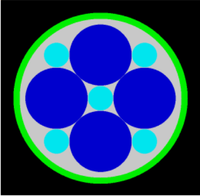
Fig. 8.1.25 Close-packed cylinders in an annulus.

Data description of Example 15.

KENO V.a:

READ GEOM
UNIT 1
CYLINDER 1 1 0.6 2P15.0
UNIT 2
CYLINDER 3 1 1.4 2P15.0
GLOBAL UNIT 3
CYLINDER 1 1 0.6 2P15.0
CYLINDER 0 1 3.6 2P15.0
HOLE 2 0.0 -2.0 0.0
HOLE 1 2.0 -2.0 0.0
HOLE 2 2.0 0.0 0.0
HOLE 1 2.0 2.0 0.0
HOLE 2 0.0 2.0 0.0
HOLE 1 -2.0 2.0 0.0
HOLE 2 -2.0 0.0 0.0
HOLE 1 -2.0 -2.0 0.0
CYLINDER  2 1 3.8 2P15.0
CUBOID    0 1 4P4.0 2P16.0
END GEOM

KENO-VI:

READ GEOM
GLOBAL UNIT 1
CYLINDER 1 0.6 2P15.0
CYLINDER 2 0.6 2P15.0 ORIGIN X=2.0  Y=-2.0
CYLINDER 3 0.6 2P15.0 ORIGIN X=2.0  Y=2.0
CYLINDER 4 0.6 2P15.0 ORIGIN X=-2.0 Y=2.0
CYLINDER 5 0.6 2P15.0 ORIGIN X=-2.0 Y=-2.0
CYLINDER 6 1.4 2P15.0 ORIGIN X=2.0
CYLINDER 7 1.4 2P15.0 ORIGIN Y=2.0
CYLINDER 8 1.4 2P15.0 ORIGIN X=-2.0
CYLINDER 9 1.4 2P15.0 ORIGIN Y=-2.0
CYLINDER 10 3.6 2P15.0
CYLINDER 11 3.8 2P15.0
CUBOID  12  4P4.0 2P16.0
MEDIA 1 1 1
MEDIA 1 1 2
MEDIA 1 1 3
MEDIA 1 1 4
MEDIA 1 1 5
MEDIA 3 1 6
MEDIA 3 1 7
MEDIA 3 1 8
MEDIA 3 1 9
MEDIA 0 1 10 -1 -2 -3 -4 -5 -6 -7 -8 -9
MEDIA 2 1 11 -10
MEDIA 0 1 12 -11
BOUNDARY  12
END GEOM

The first HOLE description in the KENO V.a input represents the bottom large rod. It takes UNIT 2 and places its ORIGIN at (0.0,-2.0,0.0) relative to the ORIGIN of UNIT 3. The second HOLE description represents the small rod to the right of the large rod just discussed. It places the origin of UNIT 1 at (2.0,-2.0,0.0) in UNIT 3. The third HOLE description represents the large rod to the right. It places the origin of UNIT 2 at (2.0,0.0,0.0) in UNIT 3. This procedure is repeated in a counterclockwise direction until all eight rods have been placed within the region that defines the inner surface of the annulus. The CYLINDER that defines the outer surface of the annulus is described after all the HOLEs for the previous region have been placed. Then the outer CUBOID is described. This example illustrates that a UNIT that is to be placed using a HOLE description need not have a CUBE or CUBOID as its last region. Note that including the central rod directly in UNIT 3 reduces the CPU time required for transport compared to the case of all 9 rods being inserted as HOLEs. It is also important that the 9 HOLEs are inserted after the void cylinder into which they are inserted. Entering the HOLEs in any other position in the input would generated region intersection errors. The order of the HOLE records in any given region is not important, as they can be interchanged with each other randomly. However, they must always appear immediately after the region in which they are placed.

The KENO-VI input does not need to use HOLEs. The first CYLINDER description in this case represents the middle small rod. The next four CYLINDER records describe the four remaining small rods surrounding the middle rod. The ORIGIN attribute is used to shift the origin of each CYLINDER to the appropriate location. The following four CYLINDER records represent the four large rods. Again, the ORIGIN attribute is used to shift the ORIGIN of each CYLINDER to the appropriate location. Only the nonzero dimensions need to be entered in the ORIGIN data. The tenth CYLINDER record is the void in the annulus that contains the rods. The last CYLINDER record defines the outer surface of the annulus. Finally, the CUBOID record describes the surrounding UNIT boundary.

In KENO-VI, holes may not extend across any array outer boundary, may not intersect with other holes, and may not cross the host UNIT outer boundary. Thus a hole may be placed so that it crosses several regions within an array. The hole description replaces the unit description within the hole domain. Since the holes are placed using the host UNIT coordinate system, the location of the hole record in the unit definition is not relevant.

An array of the arrangement shown in Fig. 8.1.25 can be easily described by altering the array description data. For example, a 5 \(\times\) 3 \(\times\) 2 array of these shapes with a center-to-center spacing of 8 cm in X and Y and 32 cm in Z can be achieved by using the following array data:

READ ARRAY  NUX=5 NUY=3 NUZ=2  FILL F3  END FILL  END ARRAY

or

READ ARRAY  NUX=5 NUY=3 NUZ=2  FILL 30*3  END FILL  END ARRAY

or

READ ARRAY  NUX=5 NUY=3 NUZ=2  LOOP  3 1 5 1 1 3 1 1 2 1  END LOOP END ARRAY

8.1.4.6.2. Nesting holes

This section illustrates how holes are nested. Holes can be nested to any level. Consider the configuration illustrated in Fig. 8.1.25 and replace the large rods with a complicated geometric arrangement. The resulting Fig. is shown in Fig. 8.1.26. Fig. 8.1.27 shows the complicated geometric arrangement that replaced the large rods of Fig. 8.1.25. Fig. 8.1.28 shows a component of the arrangement shown in Fig. 8.1.26.

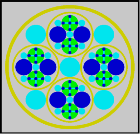
Fig. 8.1.26 Configuration using nested holes.

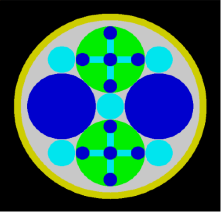
Fig. 8.1.27 Complicated geometric arrangement by Unit 7.

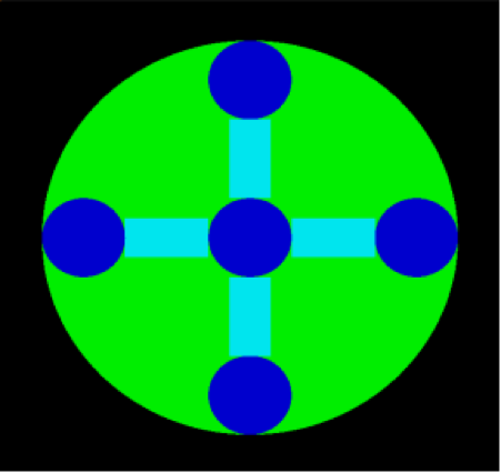
Fig. 8.1.28 Geometric component represented by Unit 4.

EXAMPLE 16. There is no predetermined preferred method to create a geometry mockup for a given physical system. The user should determine the most convenient order. To describe the configuration shown in Fig. 8.1.26 using nested HOLEs, it is likely most convenient to start the geometry mockup at the deepest nesting level, as shown in Fig. 8.1.27. The small CYLINDERs are composed of mixture 1, and they are each 0.1 cm in radius and 30 cm long. There are five small CYLINDERs used in Fig. 8.1.28. Their centers are located at (0,0,0) for the central one, at (0,-0.4,0) for the bottom one, at (0.4,0,0) for the right one, at (0,0.4,0) for the top one, and at (-0.4,0,0) for the left one. The rectangular parallelepipeds (CUBOIDs) are composed of mixture 2. Each one is 30 cm long and 0.1 cm by 0.2 cm in cross section. The large CYLINDER containing the configuration is composed of mixture 3, is 30 cm long and has a radius of 0.5 cm.

A possible geometry mockup for this system is described as follows in KENO V.a:

1. define a small cylinder to be UNIT 1,

(2) define a small CUBOID with its length in the X direction to be UNIT 2,

(3) define a small CUBOID with its length in the Y direction to be UNIT 3,

(4) define UNIT 4 to be the large cylinder and place the CYLINDERs and CUBOIDs in it using HOLEs.

UNIT 1
CYLINDER 1 1 0.1 2P15.0
UNIT 2
CUBOID 2 1 2P0.1 2P0.05 2P15.0
UNIT 3
CUBOID 2 1 2P0.05 2P0.1 2P15.0
UNIT 4
CYLINDER  1 1 0.1 2P15.0
CYLINDER  3 1 0.5 2P15.0
HOLE 1 0.0 -0.4 0.0
HOLE 1 0.4 0.0 0.0
HOLE 1 0.0 0.4 0.0
HOLE 1 -0.4 0.0 0.0
HOLE 2 -0.2 0.0 0.0
HOLE 2 0.2 0.0 0.0
HOLE 3 0.0 -0.2 0.0
HOLE 3 0.0 0.2 0.0

The first cylinder description in UNIT 4 places the central rod,

the second cylinder description in UNIT 4 places the outer cylinder,

the first HOLE places the bottom CYLINDER,

the second HOLE places the CYLINDER at the right,

the third HOLE places the top CYLINDER,

the fourth HOLE places the CYLINDER at the left,

the fifth HOLE places the left CUBOID whose length is in X,

the sixth HOLE places the right CUBOID whose length is in X,

the seventh HOLE places the bottom CUBOID whose length is in Y, and

the eighth HOLE places the top CUBOID whose length is in Y.

A possible geometry mockup for this system is described as follows in KENO-VI:

1. define UNIT 1 to contain the five small cylinders and four blocks,

2. define UNIT 2 to contain the next two larger-sized cylinders and UNIT 1 as HOLEs, and

3. define GLOBAL UNIT 3 to contain the large cylinders and UNIT 2 as HOLEs.

UNIT 1
CYLINDER  1 0.1 2P15.0
CYLINDER  2 0.1 2P15.0 ORIGIN Y=-0.4
CYLINDER  3 0.1 2P15.0 ORIGIN X=0.4
CYLINDER  4 0.1 2P15.0 ORIGIN Y=0.4
CYLINDER  5 0.1 2P15.0 ORIGIN X=-0.4
CUBOID    6 -0.3 -0.1  2P0.05 2P15.0
CUBOID    7 0.3 0.1  2P0.05 2P15.0
CUBOID    8 2P0.05 -0.3 -0.1  2P15.0
CUBOID    9 2P0.05 0.3 0.1  2P15.0
CYLINDER 10 0.5 2P15.0
MEDIA 1 1 1
MEDIA 1 1 2
MEDIA 1 1 3
MEDIA 1 1 4
MEDIA 1 1 5
MEDIA 2 1 6
MEDIA 2 1 7
MEDIA 2 1 8
MEDIA 2 1 9
MEDIA 3 1 10 -1 -2 -3 -4 -5 -6 -7 -8 -9
BOUNDARY  10

geometry record 1 places the central rod,

geometry record 2 places the bottom CYLINDER,

geometry record 3 places the CYLINDER at the right,

geometry record 4 places the top CYLINDER,

geometry record 5 places the CYLINDER at the left,

geometry record 6 places the left CUBOID whose length is in X,

geometry record 7 places the right CUBOID whose length is in X,

geometry record 8 places the bottom CUBOID whose length is in Y,

geometry record 9 places the top CUBOID whose length is in Y, and

geometry record 10 is the surrounding CYLINDER that defines the unit boundary.

In Fig. 8.1.27, the large plain cylinders are composed of mixture 1 and are 0.5 cm in radius and 30 cm long. The cylindrical component of UNIT 4 for KENO V.a or UNIT 1 for KENO-VI is the same size: an outer radius of 0.5 cm and a length of 30 cm. The small cylinders located in the interstices between the large cylinders are composed of mixture 2, are 0.2 cm in radius, and are 30 cm long. The annulus is composed of mixture 4, has a 1.3 cm inside radius and a 1.4 cm outer radius. The volume between the inner cylinders is void. The large cylinders each have a radius of 0.5 cm and are tangent. Therefore, their origins are offset from the origin of the UNIT by 0.707107. This is from X² + Y² = 1.0, where X and Y are equal.

For KENO V.a, define UNIT 5 to be the large plain cylinder, UNIT 6 to be the small cylinder, and UNIT 7 as the annulus that contains the cylinders. Its origin is at its center. The geometry mockup for this portion of the problem follows:

KENO V.a:

UNIT 5
CYLINDER  1 1 0.5 2P15.0
UNIT 6
CYLINDER  2 1 0.2 2P15.0
UNIT 7
CYLINDER  2 1 0.2 2P15.0
CYLINDER  0 1 1.3 2P15.0
HOLE      5 0.707107 0.0 0.0
HOLE      6 0.707107 0.707107 0.0
HOLE      4 0.0 0.707107 0.0
HOLE      6 -0.707107 0.707107 0.0
HOLE      5 -0.707107 0.0 0.0
HOLE      6 -0.707107 -0.707107 0.0
HOLE      4 0.0 -0.707107 0.0
HOLE      6 0.707107 -0.707107 0.0
CYLINDER  4 1 1.4 2P15.0

The first HOLE places the larger CYLINDER of mixture 1 at the right with its origin at (0.707107,0.0,0.0),

the second HOLE places the small CYLINDER in the upper right quadrant,

the third HOLE places the top CYLINDER that contains the geometric component defined in UNIT 4,

the fourth HOLE places the small CYLINDER in the upper left quadrant,

the fifth HOLE places the larger CYLINDER of mixture 1 at the left,

the sixth HOLE places the small CYLINDER in the lower lower left quadrant,

the seventh HOLE places the bottom CYLINDER that contains the geometric component defined in UNIT 4, and

the eighth HOLE places the small CYLINDER in the lower right quadrant.

The last CYLINDER defines the outer surface of the annulus.

For KENO-VI, UNIT 2 is the annulus that contains the cylinders.

KENO-VI:

UNIT 2
CYLINDER  1 0.2 2P15.0
CYLINDER  2 0.2 2P15.0 ORIGIN X=0.707107  Y=0.707107
CYLINDER  3 0.2 2P15.0 ORIGIN X=-0.707107 Y=0.707107
CYLINDER  4 0.2 2P15.0 ORIGIN X=-0.707107 Y=-0.707107
CYLINDER  5 0.2 2P15.0 ORIGIN X=0.707107  Y=-0.707107
CYLINDER  6 0.5 2P15.0 ORIGIN X=0.707107
CYLINDER  7 0.5 2P15.0 ORIGIN X=-0.707107
CYLINDER 10 1.3 2P15.0
CYLINDER 11 1.4 2P15.0
MEDIA 2 1 1
MEDIA 2 1 2
MEDIA 2 1 3
MEDIA 2 1 4
MEDIA 2 1 5
MEDIA 1 1 6
MEDIA 1 1 7
HOLE 1 ORIGIN Y=0.707107
HOLE 1 ORIGIN Y=-0.707107
MEDIA 0 1 10 -1 -2 -3 -4 -5 -6 -7
MEDIA 4 1 11 -10
BOUNDARY  11

In Unit 2 of the above KENO-VI geometry,

CYLINDER 1 places a small CYLINDER of mixture 2 at the origin,

CYLINDER 2 places the small CYLINDER of mixture 2 in the upper right quadrant,

CYLINDER 3 places the small CYLINDER of mixture 2 in the upper left quadrant,

CYLINDER 4 places the small CYLINDER of mixture 2 in the lower left quadrant,

CYLINDER 5 places the small CYLINDER of mixture 2 in the lower right quadrant,

CYLINDER 6 places the larger CYLINDER of mixture 1 at the right with its origin at (0.707107,0.0,0.0),

CYLINDER 7 places the larger CYLINDER of mixture 1 at the left with its origin at (0.0,0.707107.0.0),

CYLINDER 10 defines the inner surface of the annulus,

CYLINDER 11 defines the outer surface of the annulus and the UNIT boundary,

the first HOLE places the top CYLINDER that contains the geometric component defined in UNIT 1, and

the second HOLE places the bottom CYLINDER that contains the geometric component defined in UNIT 1.

To complete the geometry mockup, consider Fig. 8.1.26.

For KENO V.a geometry, define UNIT 8 to be a cylinder of mixture 2 having a radius of 0.6 cm and a length of 30 cm. Define UNIT 9 to be the central rod and the large annulus of 3.6 cm inner radius, 3.8 cm outer radius, and 30 cm length centered in a CUBOID having an 8 cm² cross section and being 32 cm long.

KENO V.a:

UNIT 8
CYLINDER  2 1 0.6 2P15.0
UNIT 9
CYLINDER  2 1 0.6 2P15.0
CYLINDER  0 1 3.6 2P15
HOLE   7 2.0 0.0 0.0
HOLE   8 2*2.0 0.0
HOLE   7 0.0 2.0 0.0
HOLE   8 -2.0 2.0 0.0
HOLE   7 -2.0 2*0.0
HOLE   8 2*-2.0 0.0
HOLE   7 0.0 -2.0 0.0
HOLE   8 2P2.0 0.0
CYLINDER  4 1 3.8 2P15.0
CUBOID    0 1 4P4.0 2P16.0

In UNIT 9 of the KENO V.a description, the first CYLINDER defines the rod of mixture 2, centered in the annulus. The second CYLINDER defines the void volume between the central rod and the annulus.

The first HOLE places the composite annulus of UNIT 7 to the right of the central rod,

the second HOLE places a rod defined by UNIT 8 in the upper right quadrant of the annulus,

the third HOLE places the composite annulus of UNIT 7 above the central rod,

the fourth HOLE places a rod defined by UNIT 8 in the upper left quadrant of the annulus,

the fifth HOLE places the composite annulus of UNIT 7 to the left of the central rod,

the sixth HOLE places a rod defined by UNIT 8 in the lower left quadrant,

the seventh HOLE places the composite annulus of UNIT 7 below the central rod, and

the eighth HOLE places a rod defined by UNIT 8 in the lower right quadrant.

The last CYLINDER defines the outer surface of the annulus. The outer CUBOID is the last region.

For KENO-VI geometry, define UNIT 3 to be the central rod and four outer rods of 0.6 cm radius and 30.0 cm length, and the large annulus of 3.6 cm inner radius, 3.8 cm outer radius, and 30 cm length centered in a cuboid having an 8 cm² cross section and a length of 32 cm.

KENO-VI:

GLOBAL UNIT 3
CYLINDER  1 0.6 2P15.0
CYLINDER  2 0.6 2P15.0 ORIGIN X=2.0 Y=2.0
CYLINDER  3 0.6 2P15.0 ORIGIN X=-2.0 Y=2.0
CYLINDER  4 0.6 2P15.0 ORIGIN X=-2.0 Y=-2.0
CYLINDER  5 0.6 2P15.0 ORIGIN X=2.0 Y=-2.0
CYLINDER 10 3.6 2P15.0
CYLINDER 11 3.8 2P15.0
CUBOID   12 4P4.0 2P16.0
MEDIA 2 1 1
MEDIA 2 1 2
MEDIA 2 1 3
MEDIA 2 1 4
MEDIA 2 1 5
HOLE  2 ORIGEN X=2
HOLE  2 ORIGEN Y=2
HOLE  2 ORIGEN X=-2
HOLE  2 ORIGEN Y=-2
MEDIA 0 1 10 -1 -2 -3 -4 -5
MEDIA 4 1 11 -10
MEDIA 0 1 12 -11
BOUNDARY  12

In UNIT 3 of the above KENO-VI description,

CYLINDER 1 defines the rod of mixture 2, centered in the annulus,

CYLINDER 2 places a rod of mixture 2 in the upper right quadrant of the annulus,

CYLINDER 3 places a rod of mixture 2 in the upper left quadrant of the annulus,

CYLINDER 4 places a rod of mixture 2 in the lower left quadrant,

CYLINDER 5 places a rod of mixture 2 in the lower right quadrant,

CYLINDER 10 defines the void volume between the central rod and the annulus,

CYLINDER 11 defines the outer surface of the annulus,

CUBOID 12 defines the unit boundary,

the first HOLE places UNIT 2 to the right of the central rod,

the second HOLE places UNIT 2 above the central rod,

the third HOLE places UNIT 2 to the left of the central rod, and

the fourth HOLE places UNIT 2 below the central rod.

This problem illustrates three levels of HOLE nesting. The total input data for the problem is given below. The geometry description accurately recreates the geometry arrangement of Fig. 8.1.26. The 2D color plot output is shown in Fig. 8.1.29.

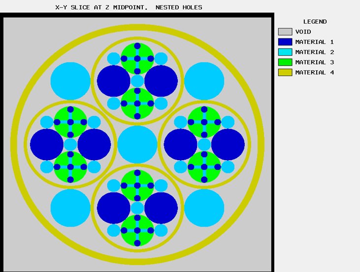
Fig. 8.1.29 Color plot of nested holes example problem.

KENO V.a:

NESTED HOLES SAMPLE

READ GEOM
UNIT 1
CYLINDER 1 1 0.1 2P15.0
UNIT 2
CUBOID 2 1 2P0.1 2P0.05 2P15.0
UNIT 3
CUBOID 2 1 2P0.05 2P0.1 2P15.0
UNIT 4
CYLINDER 1 1 0.1 2P15.0
CYLINDER 3 1 0.5 2P15.0
HOLE 1  0.0 -0.4 0.0
HOLE 1  0.4  0.0 0.0
HOLE 1  0.0  0.4 0.0
HOLE 1 -0.4  0.0 0.0
HOLE 2 -0.2  0.0 0.0
HOLE 2  0.2  0.0 0.0
HOLE 3  0.0 -0.2 0.0
HOLE 3  0.0  0.2 0.0
UNIT 5
CYLINDER 1 1 0.5 2P15.0
UNIT 6
CYLINDER 2 1 0.2 2P15.0
UNIT 7
CYLINDER 2 1 0.2 2P15.0
CYLINDER 0 1 1.3 2P15.0
HOLE 5 0.707107 2*0.0
HOLE 6 0.707107 0.707107 0.0
HOLE 4 0.0 0.707107 0.0
HOLE 6 -0.707107 0.707107 0.0
HOLE 5 -0.707107 0.0 0.0
HOLE 6 -0.707107 -0.707107 0.0
HOLE 4 0.0 -0.707107 0.0
HOLE 6 0.707107 -0.707107 0.0
CYLINDER 4 1 1.4 2P15.0
UNIT 8
CYLINDER 2 1 0.6 2P15.0
GLOBAL UNIT 9
CYLINDER 2 1 0.6 2P15.0
CYLINDER 0 1 3.6 2P15.0
HOLE 7 2.0 0.0 0.0
HOLE 8 2*2.0 0.0
HOLE 7 0.0 2.0 0.0
HOLE 8 -2.0 2.0 0.0
HOLE 7 -2.0 2*0.0
HOLE 8 2*-2.0 0.0
HOLE 7 0.0 -2.0 0.0
HOLE 8 2P2.0 0.0
CYLINDER 4 1 3.8 2P15.0
CUBOID 0 1 4P4.0 2P16.0
END GEOM
READ PLOT
  TTL='X-Y SLICE AT Z MIDPOINT. NESTED HOLES'
  XUL=-0.1  YUL=8.1 ZUL=16.0
  XLR=8.1 YLR=-0.1 ZLR=16
  UAX=1.0 VDN=-1.0  NAX=260 NCH=' *-.X' SCR=NO
END PLOT
END DATA
END

KENO-VI:

READ GEOM
UNIT 1
CYLINDER  1 0.1 2P15.0
CYLINDER  2 0.1 2P15.0 ORIGIN Y=-0.4
CYLINDER  3 0.1 2P15.0 ORIGIN X=0.4
CYLINDER  4 0.1 2P15.0 ORIGIN Y=0.4
CYLINDER  5 0.1 2P15.0 ORIGIN X=-0.4
CUBOID    6 -0.3 -0.1  2P0.05 2P15.0
CUBOID    7 0.3 0.1  2P0.05 2P15.0
CUBOID    8 2P0.05 -0.3 -0.1  2P15.0
CUBOID    9 2P0.05 0.3 0.1  2P15.0

CYLINDER 10 0.5 2P15.0
MEDIA 1 1 1 -6 -7 -8 -9
MEDIA 1 1 2 -8
MEDIA 1 1 3 -7
MEDIA 1 1 4 -9
MEDIA 1 1 5 -6
MEDIA 2 1 6 -1 -5
MEDIA 2 1 7 -1 -3
MEDIA 2 1 8 -1 -2
MEDIA 2 1 9 -1 -4
MEDIA 3 1 -1 -2 -3 -4 -5 -6 -7 -8 -9 10
BOUNDARY  10
UNIT 2
CYLINDER  1 0.2 2P15.0
CYLINDER  2 0.2 2P15.0 ORIGIN X=0.707107  Y=0.707107
CYLINDER  3 0.2 2P15.0 ORIGIN X=-0.707107 Y=0.707107
CYLINDER  4 0.2 2P15.0 ORIGIN X=-0.707107 Y=-0.707107
CYLINDER  5 0.2 2P15.0 ORIGIN X=0.707107  Y=-0.707107
CYLINDER  6 0.5 2P15.0 ORIGIN X=0.707107
CYLINDER  7 0.5 2P15.0 ORIGIN X=-0.707107
CYLINDER 10 1.3 2P15.0
CYLINDER 11 1.4 2P15.0
MEDIA 2 1 1
MEDIA 2 1 2
MEDIA 2 1 3
MEDIA 2 1 4
MEDIA 2 1 5
MEDIA 1 1 6
MEDIA 1 1 7
HOLE  1 ORIGIN Y=0.707107
HOLE  1 ORIGIN Y=-0.707107
MEDIA 0 1 10 -1 -2 -3 -4 -5 -6 -7
MEDIA 4 1 11 -10
BOUNDARY  11
GLOBAL UNIT 3
CYLINDER  1 0.6 2P15.0
CYLINDER  2 0.6 2P15.0 ORIGIN X=2.0  Y=2.0
CYLINDER  3 0.6 2P15.0 ORIGIN X=-2.0 Y=2.0
CYLINDER  4 0.6 2P15.0 ORIGIN X=-2.0 Y=-2.0
CYLINDER  5 0.6 2P15.0 ORIGIN X=2.0  Y=-2.0
CYLINDER 10 3.6 2P15.0
CYLINDER 11 3.8 2P15.0
CUBOID   12 4P4.0 2P16.0
MEDIA 2 1 1
MEDIA 2 1 2
MEDIA 2 1 3
MEDIA 2 1 4
MEDIA 2 1 5
HOLE 2 ORIGIN X=2
HOLE 2 ORIGIN Y=2
HOLE 2 ORIGIN X=-2
HOLE 2 ORIGIN Y=-2
MEDIA 0 1 10 -1 -2 -3 -4 -5
MEDIA 4 1 11 -10
MEDIA 0 1 12 -11
BOUNDARY  12
END GEOM
READ PLOT
  TTL='X-Y SLICE AT Z MIDPOINT. NESTED HOLES'
  XUL=-4.1  YUL=4.1 ZUL=0.0
  XLR=4.1 YLR=-4.1 ZLR=0
  UAX=1.0 VDN=-1.0  NAX=800
END PLOT
END DATA
END

8.1.4.6.3. Multiple arrays

EXAMPLE 17. Sect. 8.1.4.6 demonstrates how UNITs are composed of geometry regions and how these UNITs can be stacked in an ARRAY. This same procedure can be extended to create multiple ARRAYs. Furthermore, ARRAYs can be used as building blocks within other ARRAYs.

Consider Sample Problem 19 from Sect. 8.1.8.3. This problem is a critical experiment consisting of a composite array [Tho64, Tho73] of four highly enriched uranium metal cylinders and four cylindrical Plexiglas containers filled with uranyl nitrate solution. A photograph of the experiment is given in Fig. 8.1.235. The coordinate system is defined to be Z up the page, Y across the page, and X out of the page.

The Plexiglas containers have an inside radius of 9.525 cm and an outside radius of 10.16 cm. The inside height is 17.78 cm, and the outside height is 19.05 cm. Four of these containers are stacked with a center-to-center spacing of 21.75 cm in the Y direction and 20.48 cm in the Z direction (vertical). This arrangement of four Plexiglas containers can be described as follows: mixture 2 is the uranyl nitrate and mixture 3 is Plexiglas, so the Plexiglas container with its appropriate spacing CUBOID can be described as UNIT 1. This considers the ARRAY to be bare and suspended with no supports.

KENO V.a:

UNIT 1
CYLINDER  2 1 9.525  2P8.89
CYLINDER  3 1 10.16  2P9.525
CUBOID    0 1 4P10.875  2P10.24

KENO-VI:

UNIT 1
CYLINDER 1  9.525  2P8.89
CYLINDER 2  10.16  2P9.525
CUBOID  3   4P10.875  2P10.24
MEDIA 2 1 1
MEDIA 3 1 2 -1
MEDIA 0 1 3 -2
BOUNDARY  3

The ARRAY of four Plexiglas containers can be described as ARRAY 1 in the array data as follows:

ARA=1 NUX=1 NUY=2 NUZ=2 FILL F1 END FILL

The four metal cylinders, comprised of mixture 1, each have a radius of 5.748 cm and are 10.765 cm tall. They have a center-to-center spacing of 13.18 cm in the Y direction and 12.45 cm in the Z direction (vertical). Thus, one of the metal cylinders with its appropriate spacing CUBOID can be described as UNIT 2. This ARRAY is also considered to be bare and unsupported.

KENO V.a:

UNIT 2
CYLINDER 1 1  5.748 2P5.3825
CUBOID   0 1  4P6.59 2P6.225

KENO-VI:

UNIT 2
CYLINDER 1 5.748 2P5.3825
CUBOID   2   4P6.59 2P6.225
MEDIA 1 1 1
MEDIA 0 1 2 -1
BOUNDARY  2

The array of four metal cylinders can be described as ARRAY 2 in the array data.

ARA=2 NUX=1 NUY=2 NUZ=2 FILL F2 END FILL

Now two ARRAYs have been described. The overall dimensions of the ARRAY of Plexiglas containers are 21.75 cm in X, 43.5 cm in Y, and 40.96 cm in Z. The overall dimensions of the ARRAY of metal cylinders are 13.18 cm in X, 26.36 cm in Y, and 24.9 cm in Z.

In order to describe the composite ARRAY, these two ARRAYs must be positioned within UNITs and stacked together into one ARRAY. In order for them to be stacked into one ARRAY, the adjacent faces must match. This is accomplished by defining a UNIT 3 which contains ARRAY 1, the ARRAY of Plexiglas solution containers. The overall dimensions of this UNIT are 21.75 cm in X, 43.5 cm in Y, and 40.96 cm in Z. These dimensions are calculated by the code and need not be specified. UNIT 3 is defined as follows:

KENO V.a:

UNIT 3
ARRAY 1  3*0.0

KENO-VI:

UNIT 3
CUBOID  1 2P10.875 2P21.75 2P20.48
ARRAY 1 1 PLACE 1 1 1 0.0 -10.875 -10.24
BOUNDARY  1

The ARRAY of metal cylinders will be defined to be UNIT 4. However, this ARRAY is 17.14 cm smaller in the Y and 16.06 cm smaller in the Z dimensions than the ARRAY of Plexiglas UNITs. Therefore, a void region must be placed around the ARRAY in those directions so UNIT 4 and UNIT 3 will be the same size in Y and Z.

KENO V.a:

UNIT 4
ARRAY  2  3*0.0
REPLICATE  0 1 2*0.0  2*8.57  2*8.03  1

KENO-VI:

Now that UNIT 3 and UNIT 4 have been defined, they must be placed in the global or universe ARRAY to define the physical arrangement of the eight pieces. This procedure is implemented via a GLOBAL ARRAY in KENO V.a, while KENO-VI uses a GLOBAL UNIT 3 as follows:

KENO V.a:

GBL=3  ARA=3  NUX=2  NUY=1  NUZ=1  FILL  4 3  END FILL

KENO-VI:

GLOBAL UNIT 5
CUBOID 1 34.93 0.0 43.5 0.0 40.96 0.0
ARRAY 3 1 PLACE 1 1 1 6.59 21.75 20.48
BOUNDARY  1

The description of ARRAY 3 in KENO-VI is identical to that shown for KENO V.a.

This completes the geometry description for the problem. The complete geometry input description for the problem is given below.

KENO V.a:

=KENOVA
SAMPLE PROBLEM 19 4 AQUEOUS 4 METAL ARRAY OF ARRAYS
READ PARAM  LIB=4  RUN=NO END PARAM
READ MIXT SCT=1
     MIX=1
  1092238     3.2275e-3
  1092235     4.4802e-2
     MIX=2
  20011023    5.81e-2
  2007014     1.9753e-3
  2008016     3.6927e-2
  20092235    9.8471e-4
  20092238    7.7697e-5
     MIX=3
  11006012    3.5552e-2
  11011023    5.6884e-2
  11008016    1.4221e-2
END MIXT
READ GEOM
UNIT 1
  CYLINDER  2 1 9.525 8.89 -8.89
  CYLINDER  3 1 10.16 2P9.525
  CUBOID  0 1 4P10.875 2P10.24
UNIT 2
  CYLINDER  1 1 5.748 2P5.3825
  CUBOID  0 1 4P6.59 2P6.225
UNIT 3
  ARRAY 1 3*0.0
UNIT 4
  ARRAY 2 3*0.0
  REPLICATE 0 1 2*0.0 2*8.57 2*8.03 1
END GEOM
READ ARRAY
  ARA=1 NUX=1 NUY=2 NUZ=2                FILL F1 END FILL
  ARA=2 NUX=1 NUY=2 NUZ=2                FILL F2 END FILL
  GBL=3 ARA=3 NUX=2 NUY=1 NUZ=1   FILL 4 3 END FILL
END ARRAY
  READ PLOT TTL='X-Y SLICE AT Z=10.24'
  XUL=-1.0    YUL=44.5 ZUL=10.24
  XLR=35.93 YLR=-1.0  ZLR=10.24
  UAX=1.0 VDN=-1.0 NAX=640 PIC=MIX END
  TTL='X-Z SLICE AT Y=10.875'
  XUL=-1.0 YUL=10.875 ZUL=41.96 XLR=35.93 YLR=10.875 ZLR=-1.0
  UAX=1.0 WDN=-1.0 PIC=MIX END  END PLOT
END DATA
END

KENO-VI:

=KENO-VI
SAMPLE PROBLEM 19 4 AQUEOUS 4 METAL ARRAY OF ARRAYS
READ PARAM
  LIB=4 FLX=YES FDN=YES NUB=YES SMU=YES MKP=YES MKU=YES FMP=YES FMU=YES
END PARAM
READ MIXT
  SCT=2
  MIX=1
      1092234 4.82717E-04
      1092235 4.47971E-02
      1092236 9.57233E-05
      1092238 2.65767E-03
  MIX=2
      2001001 5.77931E-02
      2007014 2.13092E-03
      2008016 3.74114E-02
      2092234 1.06784E-05
      2092235 9.84602E-04
      2092236 5.29386E-06
      2092238 6.19414E-05
  MIX=3
      11001001 5.67873E-02
      11006000 3.54921E-02
      11008016 1.41968E-02
END MIXT
READ GEOM
UNIT 1
  CYLINDER 1  9.525  2P8.89
  CYLINDER 2  10.16  2P9.525
  CUBOID   3  4P10.875  2P10.24
  MEDIA 2 1 1
  MEDIA 3 1 2 -1
  MEDIA 0 1 3 -2
  BOUNDARY  3
UNIT 2
  CYLINDER  1 5.748 2P5.3825
  CUBOID    2 4P6.59 2P6.225
  MEDIA 1 1 1
  MEDIA 0 1 2 -1
  BOUNDARY  2
UNIT 3
  CUBOID 1 2P10.875 2P21.75 2P20.48
  ARRAY 1 1 PLACE 1 1 1 0.0 -10.875 -10.24
  BOUNDARY  1
UNIT 4
  CUBOID 1 2P6.59 2P13.18 2P12.45
  CUBOID 2 2P6.59 2P21.75 2P20.48
  ARRAY  2  1 PLACE 1 1 1 0.0 -6.59 -6.225
  MEDIA 0 1 2 -1
  BOUNDARY
GLOBAL UNIT 5
  CUBOID 1 34.93 0.0 43.5 0.0 40.96 0.0
  ARRAY 3 1 PLACE 1 1 1 6.59 21.75 20.48
  BOUNDARY  1
END GEOM
READ ARRAY
  ARA=1 NUX=1 NUY=2 NUZ=2                 FILL F1 END FILL
  ARA=2 NUX=1 NUY=2 NUZ=2                 FILL F2 END FILL
  GBL=3 ARA=3 NUX=2 NUY=1 NUZ=1    FILL 4 3 END FILL
END ARRAY
READ PLOT TTL='X-Y SLICE AT Z=10.24'
  XUL=-1.0 YUL=44.5 ZUL=10.24
  XLR=35.93 YLR=-1.0 ZLR=10.24
  UAX=1.0 VDN=-1.0 NAX=130 NCH=' *.-' PIC=MIX END
  TTL='X-Z SLICE AT Y=10.875'
  XUL=-1.0 YUL=10.875 ZUL=41.96
  XLR=35.93 YLR=10.875 ZLR=-1.0
  UAX=1.0 WDN=-1.0 PIC=MIX END
END PLOT
END DATA
END

A plot of an X-Y slice taken through the bottom layer of the array is shown in Fig. 8.1.30. A plot of an X-Z slice taken through the +Y half of the array is shown in Fig. 8.1.31. These plots were used to verify the geometry mockup.

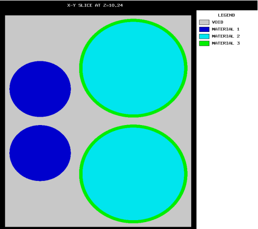
Fig. 8.1.30 X-Y plot of mixed array.

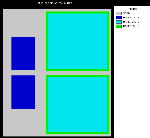
Fig. 8.1.31 X-Z plot of mixed array.

STORAGE ARRAY

EXAMPLE 18. Consider a storage array of highly enriched uranium buttons, each 1 in. tall and 4 in. in diameter. These buttons are stored on stainless steel shelves with a center-to-center spacing of 60.96 cm (2 ft) between them in the Y direction, and only one button on each shelf in the X direction. The shelves are 0.635 cm (¹/₄in.) thick (Z dimension), 45.72 cm (18 in.) wide (X dimension), 609.6 cm (20 ft) long (Y dimension), and are 45.72 cm (18 in.) from the top of a shelf to the bottom of the shelf above it. Each rack of storage shelves is four shelves high, with the first shelf being 15.24 cm (6 in.) above the floor. The storage room is 586.56 cm (19.5 ft) in the X direction by 1293.44 cm (43 ft) in the Y direction with 365.76 cm (12 ft. ) ceilings in the Z direction. The walls, ceiling, and floor are composed of concrete, 30.48 cm (1 ft) thick. All the aisles between the storage racks are 91.44 cm (3 ft) wide. The racks are arranged with their length in the Y direction and an aisle between them. The arrays of racks are arranged with two in the Y direction and five in the X direction. Mixture 1 is the uranium metal, mixture 2 is the stainless steel, and mixture 3 is the concrete.

The metal button and its center-to-center spacing are described first. The void vertical spacing has arbitrarily been chosen to extend from the bottom of the button to the next shelf above the button. The shelf of stainless steel is described under the button.

KENO V.a:

UNIT 1
COM='METAL BUTTONS'
CYLINDER 1 1 5.08 2.54 0.0
CUBOID  0 1 2P22.86 2P30.48 45.72 0.0
CUBOID  2 1 2P22.86 2P30.48 45.72 -0.635

KENO-VI:

ARRAY 1 creates an ARRAY of these buttons that fills one shelf. UNIT 2 then contains one of the shelves shown in Fig. 8.1.32.

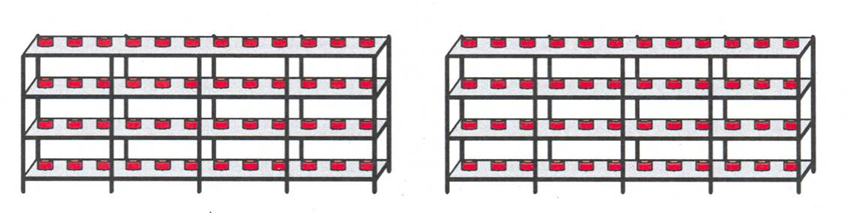
Fig. 8.1.32 Two racks of uranium buttons.

KENO V.a:

ARA=1 COM='SINGLE SHELF CONTAINING 10 METAL BUTTONS'
      NUX=1 NUY=10 NUZ=1 FILL F1 END FILL

UNIT 2
COM='SINGLE SHELF (1 X 10 X 1 ARRAY OF METAL BUTTONS ON A SHELF)'
ARRAY 1 3*0.0

KENO-VI:

ARA=1  NUX=1  NUY=10  NUZ=1  FILL  F1  END FILL

UNIT 2
CUBOID 1 45.72 0.0 609.60 0.0 46.355 0.0
ARRAY  1  1  PLACE  1  1  1  22.86  30.48  0.635
BOUNDARY  1

Note

The origin of UNIT 2 is on the bottom of the bottom shelf; it has been moved from the bottom of the button. The X and Y position of the origin is at the front, left-hand corner of the bottom of this lowest shelf.

Stack four UNIT 2s vertically to obtain one of the racks shown in Fig. 8.1.32. One rack is defined by array 2.

ARA=2 COM='SINGLE RACK OF 4 SHELVES'

NUX=1 NUY=1 NUZ=4 FILL F2 END FILL

Generate a UNIT 3 that contains a rack of shelves and a UNIT 4 that is the aisle between the ends of the two racks in the Y direction.

KENO V.a:

UNIT 3
COM='SINGLE RACK (4 SHELVES TALL)'
ARRAY 2 3*0.0

UNIT 4
COM='CENTRAL AISLE UNIT SAME HEIGHT AS 4 SHELVES'
CUBOID 0 1 2P22.86 2P45.72 185.42 0.0

KENO-VI:

UNIT 3
CUBOID 1 45.72 0.0 609.60 0.0 185.42 0.0
ARRAY  2 1 PLACE 1 1 1 3*0.0
BOUNDARY  1
UNIT 4
CUBOID  1  2P22.86  2P45.72  185.42  0.0
MEDIA 0 1 1
BOUNDARY  1

Stack UNITs 3 and 4 together in the Y direction to create UNIT 5 which contains both racks in the Y direction and the aisle between them. This configuration is shown in Fig. 8.1.32.

KENO V.a:

ARA=3 COM='TWO RACKS END TO END WITH CENTRAL AISLE'
      NUX=1 NUY=3 NUZ=1 FILL 3 4 3 END FILL

UNIT 5
COM='SET OF TWO RACKS END TO END SEPARATED BY THE CENTRAL AISLE'
ARRAY 3 3*0.0

KENO-VI:

ARA=3  NUX=1  NUY=3  NUZ=1  FILL  3 4 3  END FILL

UNIT 5
CUBOID 1 45.72 0.0 1310.64 0.0 185.42 0.0
ARRAY 3 1 PLACE 1 1 1 3*0.0
BOUNDARY  1

Create a UNIT 6, which is an aisle 91.44 cm (3 ft) wide in the X direction and 1310.64 cm (43 ft) in the Y direction (full length of the room).

KENO V.a:

UNIT 6
COM='AISLE BETWEEN ADJACENT SETS OF TWO RACKS & CENTRAL AISLE (UNITS 5)'
CUBOID 0 1 91.44 0.0 1310.64 0.0 185.42 0.0

KENO-VI:

UNIT 6
CUBOID 1 91.44 0.0  1310.64 0.0  185.42 0.0
MEDIA 0 1 1
BOUNDARY  1

Stack UNITs 5 and 6 in the X direction to achieve the array of racks in the room. Then put the 6 in. spacing below the bottom of the racks, the spacing between the top of the top rack and the ceiling, and add the concrete floor, walls, and ceiling around the array. ARRAY 4 describes the array of racks in the room. ARRAY record (first CUBOID description in KENO-VI) encompasses this ARRAY, and the first REFLECTOR (second CUBOID in KENO-VI) descriptions are used to add the spacing between the top rack and the ceiling. The last two REFLECTOR (CUBOIDs 3 through 9 in KENO-VI) descriptions add the ceiling, walls, and floor in 5.0 cm increments to bias the concrete. A perspective of the room is shown in Fig. 8.1.33.

KENO V.a:

ARA=4 COM='ENTIRE STORAGE ARRAY'
      NUX=9 NUY=1 NUZ=1 FILL 5 6 3Q2 5 END FILL
GLOBAL
UNIT 7
COM='STORAGE ARRAY IN THE ROOM WITH WALLS, FLOOR AND CEILING'
ARRAY  4  3*0.0
REFLECTOR   0  1  4*0.0  165.1  15.24  1
REFLECTOR  3  2  6*5.0  6
REFLECTOR  3  8  6*0.48  1

KENO-VI:

GBL=4  ARA=4  NUX=9  NUY=1  NUZ=1  FILL 5 6  3Q2  5  END FILL

GLOBAL UNIT  7
CUBOID 1 594.36   0.0  1310.64   0.0  185.42   0.0
CUBOID 2 594.36   0.0  1310.64   0.0  350.52 -15.24
CUBOID 3 599.36  -5.00 1315.64  -5.00 355.52 -20.24
CUBOID 4 604.36 -10.00 1320.64 -10.00 360.52 -25.24
CUBOID 5 609.36 -15.00 1325.64 -15.00 365.52 -30.24
CUBOID 6 614.36 -20.00 1330.64 -20.00 370.52 -35.24
CUBOID 7 619.36 -25.00 1335.64 -25.00 375.52 -40.24
CUBOID 8 624.36 -30.00 1340.64 -30.00 380.52 -45.24
CUBOID 9 624.84 -30.48 1341.12 -30.48 381.00 -45.72
ARRAY  4 1 PLACE 1 1 1 3*0.0
MEDIA 0 1 2 -1
MEDIA 3 2 3 -2
MEDIA 3 3 4 -3
MEDIA 3 4 5 -4
MEDIA 3 5 6 -5
MEDIA 3 6 7 -6
MEDIA 3 7 8 -7
MEDIA 3 8 9 -8
BOUNDARY  9

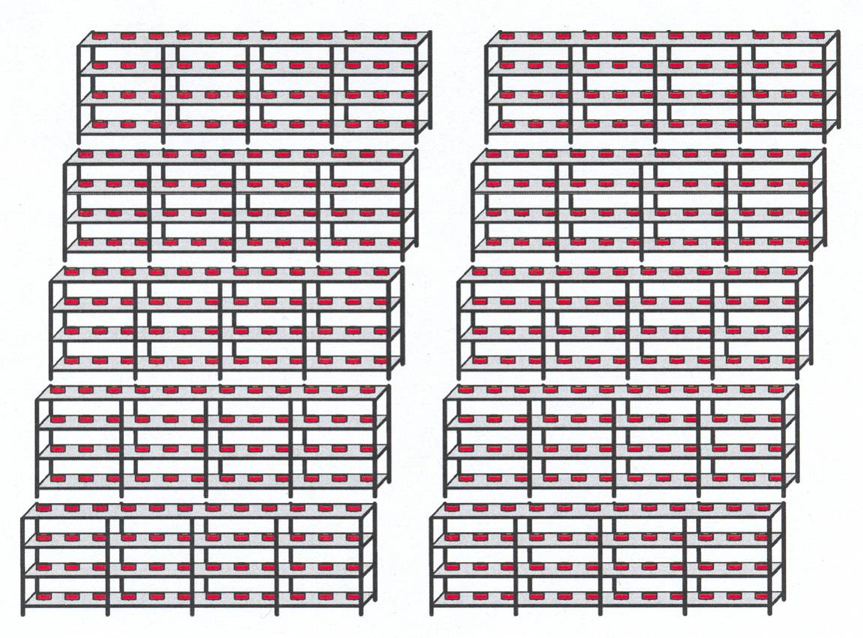
Fig. 8.1.33 Entire storage array in the room.

The complete input for this room is given below: The plots for this problem must be quite large in order to see all the detail because the array is sparse and the shelves are thin. Therefore, the plots for this system are not included as Fig.s. The user can generate the plots if it is desirable to see them. The nuclide IDs used in this problem are for the 16-group Hansen-Roach working format library, which is no longer distributed with SCALE.

KENO V.a:

=KENO5A
STORAGE ARRAY
READ PARAMETERS  FDN=YES LIB=41
END PARAMETERS
READ MIXT  SCT=1  MIX=1 92500 4.48006e-2  92800 2.6578e-3  92400 4.827e-4
92600 9.57e-5  MIX=2 200 1.0 MIX=3 301 1 END MIXT
READ GEOMETRY
UNIT 1
COM='METAL BUTTONS'
CYLINDER 1 1 5.08 2.54 0.0
CUBOID  0 1 2P22.86 2P30.48 45.72 0.0
CUBOID  2 1 2P22.86 2P30.48 45.72 -0.635
UNIT 2
COM='SINGLE SHELF (1 X 10 X 1 ARRAY OF METAL BUTTONS ON A SHELF)'
ARRAY 1 3*0.0
UNIT 3
COM='SINGLE RACK (4 SHELVES TALL)'
ARRAY 2 3*0.0
UNIT 4
COM='CENTRAL AISLE UNIT SAME HEIGHT AS 4 SHELVES'
CUBOID 0 1 2P22.86 2P45.72 185.42 0.0
UNIT 5
COM='SET OF TWO RACKS END TO END SEPARATED BY THE CENTRAL AISLE'
ARRAY 3 3*0.0
UNIT 6
COM='AISLE BETWEEN ADJACENT SETS OF TWO RACKS & CENTRAL AISLE (UNITS 5)'
CUBOID 0 1 91.44 0.0 1310.64 0.0 185.42 0.0
GLOBAL
UNIT 7
COM='STORAGE ARRAY IN THE ROOM WITH WALLS, FLOOR AND CEILING'
ARRAY 4 3*0.0
REFLECTOR 0 1 4*0.0 165.1 15.24 1
REFLECTOR 3 2 6*5.0    6
REFLECTOR 3 8 6*0.48  1
END GEOMETRY
READ ARRAY
ARA=1 COM='SINGLE SHELF CONTAINING 10 METAL BUTTONS'
      NUX=1 NUY=10 NUZ=1 FILL F1 END FILL
ARA=2 COM='SINGLE RACK OF 4 SHELVES'
      NUX=1 NUY=1 NUZ=4 FILL F2 END FILL
ARA=3 COM='TWO RACKS END TO END WITH CENTRAL AISLE'
      NUX=1 NUY=3 NUZ=1 FILL 3 4 3 END FILL
ARA=4 COM='ENTIRE STORAGE ARRAY'
      NUX=9 NUY=1 NUZ=1 FILL 5 6 3Q2 5 END FILL
END ARRAY
READ BIAS ID=301 2 8 END BIAS
READ START NST=5  NBX=5 END START
READ PLOT TTL='X-Z SLICE AT Y=30.48 WITH Z ACROSS AND X DOWN'
XUL=594.8 YUL=30.48 ZUL=-1.0 XLR=-0.5 YLR=30.48 ZLR=186.0
WAX=1.0 UDN=-1.0 NAX=640  END
TTL='Y-Z SLICE OF LEFT RACKS, X=22.86 WITH Z ACROSS AND Y DOWN'
XUL=22.86 YUL=1311.0 ZUL=-0.5 XLR=22.86 YLR=-3.0 ZLR=186.0
WAX=1.0 VDN=-1.0 NAX=640 END
TTL='X-Y SLICE OF ROOM THROUGH SHELF Z=0.3175 WITH X ACROSS AND Y DOWN'
XUL=-1.0 YUL=1312.0 ZUL=0.3175 XLR=596.0 YLR=-2.5 ZLR=0.3175
UAX=1.0 VDN=-1.0 NAX=320 END
END PLOT
END DATA
END

KENO-VI:

=KENOVI
STORAGE ARRAY
READ PARAMETERS  FDN=YES LIB=41  END PARAMETERS
READ MIXT  SCT=1
MIX=1 92500 4.48006e-2  92800 2.6578e-3  92400 4.827e-4  92600 9.57e-5
MIX=2 200 1.0 MIX=3 301 1
END MIXT
READ GEOMETRY
UNIT 1
CYLINDER 1  5.08  2.54  0.0
CUBOID   2   2P22.86   2P30.48  45.72  0.0
CUBOID   3   2P22.86   2P30.48  45.72  -.635
MEDIA 1 1 1
MEDIA 0 1 2 -1
MEDIA 2 1 3 -2
BOUNDARY  3
UNIT 2
CUBOID 1 45.72 0.0 609.60 0.0 46.355 0.0
ARRAY  1  1  PLACE  1  1  1  22.86  30.48  0.635
BOUNDARY  1
UNIT 3
CUBOID 1 45.72 0.0 609.60 0.0 185.42 0.0
ARRAY 2 1 PLACE 1 1 1 3*0.0
BOUNDARY  1
UNIT 4
CUBOID  1  2P22.86  2P45.72  185.42  0.0
MEDIA 0 1 1
BOUNDARY  1
UNIT 5
CUBOID 1 45.72 0.0 1310.64 0.0 185.42 0.0
ARRAY 3 1 PLACE 1 1 1 3*0.0
BOUNDARY  1
UNIT 6
CUBOID 1 91.44 0.0  1310.64 0.0  185.42 0.0
MEDIA 0 1 1
BOUNDARY  1
GLOBAL UNIT  7
CUBOID 1 594.36    0.0 1310.64    0.0 185.42    0.0
CUBOID 2 594.36    0.0 1310.64    0.0 350.52 -15.24
CUBOID 3 599.36  -5.00 1315.64  -5.00 355.52 -20.24
CUBOID 4 604.36 -10.00 1320.64 -10.00 360.52 -25.24
CUBOID 5 609.36 -15.00 1325.64 -15.00 365.52 -30.24
CUBOID 6 614.36 -20.00 1330.64 -20.00 370.52 -35.24
CUBOID 7 619.36 -25.00 1335.64 -25.00 375.52 -40.24
CUBOID 8 624.36 -30.00 1340.64 -30.00 380.52 -45.24
CUBOID 9 624.84 -30.48 1341.12 -30.48 381.00 -45.72
ARRAY  4 1 PLACE 1 1 1 3*0.0
MEDIA 0 1 2 -1
MEDIA 3 2 3 -2
MEDIA 3 3 4 -3
MEDIA 3 4 5 -4
MEDIA 3 5 6 -5
MEDIA 3 6 7 -6
MEDIA 3 7 8 -7
MEDIA 3 8 9 -8
BOUNDARY  9
END GEOMETRY
READ ARRAY
ARA=1 NUX=1 NUY=10 NUZ=1 FILL F1 END FILL
ARA=2 NUX=1 NUY=1 NUZ=4 FILL F2 END FILL
ARA=3 NUX=1 NUY=3 NUZ=1 FILL 3 4 3 END FILL
GBL=4 ARA=4 NUX=9 NUY=1 NUZ=1 FILL 5 6 3Q2 5 END FILL
END ARRAY
READ BIAS ID=301 2 8 END BIAS
READ START NST=5 NBX=5 END START
READ PLOT PLT=YES TTL='X-Z SLICE AT Y=30.48 WITH Z ACROSS AND X DOWN'
XUL=594.8 YUL=30.48 ZUL=-1.0 XLR=-0.5 YLR=30.48 ZLR=186.0
WAX=1.0 UDN=-1.0 NAX=640  END
TTL='Y-Z SLICE OF LEFT RACKS, X=22.86 WITH Z ACROSS AND Y DOWN'
XUL=22.86 YUL=1311.0 ZUL=-0.5 XLR=22.86 YLR=-3.0 ZLR=186.0
WAX=1.0 VDN=-1.0 NAX=640 END
TTL='X-Y SLICE OF ROOM THROUGH SHELF Z=0.3175 WITH X ACROSS AND Y DOWN'
XUL=-1.0 YUL=1312.0 ZUL=0.3175 XLR=596.0 YLR=-2.5 ZLR=0.3175
UAX=1.0 VDN=-1.0 NAX=320 END
END PLOT
END DATA
END

8.1.4.6.4. Arrays and holes

Sect. 8.1.4.6.1 and Sect. 8.1.4.6.2 describe the use of HOLEs, and Sect. 8.1.4.6.3 describes multiple ARRAYs and ARRAYs of ARRAYs. HOLEs can be used to place ARRAYs at locations in other UNITs. This section contains examples to illustrate the combined use of ARRAYs and HOLEs.

EXAMPLE 19. A SIMPLE CASK

This example consists of cylindrical mild steel container with an inside radius of 4.15 cm and a radial wall thickness of 0.45 cm. The thickness of the ends of the container is 1.27 cm, and the inside height is 10.1 cm. Highly enriched uranium rods 1 cm in diameter and 10 cm long are banded together into square bundles of four. These bundles are then positioned in the mild steel container as shown in Fig. 8.1.34. The rods sit on the floor of the container and have a 0.1 cm gap between their tops and the top of the container.

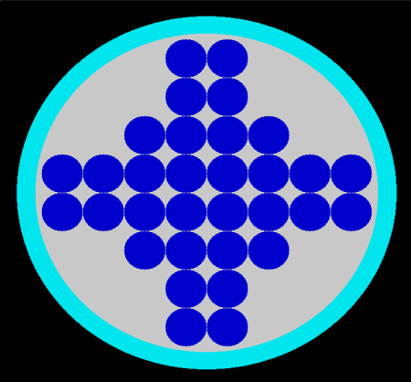
Fig. 8.1.34 Uranium rods in a cylindrical container.

To generate the geometry description for this system, UNIT 1 is defined as one uranium rod and its associated square-pitch close-packed spacing region.

KENO V.a:

UNIT 1
CYLINDER  1 1  0.5  2P5.0
CUBOID    0 1  4P0.5  2P5.0

KENO-VI:

UNIT 1
CYLINDER 1 0.5  2P5.0
CUBOID   2   4P0.5  2P5.0
MEDIA 1 1 1
MEDIA 0 1 2 -1
BOUNDARY  2

From here, the geometry description diverges between KENO V.a and KENO-VI.

KENO V.a:

ARRAY 1 is defined to be the central square ARRAY consisting of four bundles of rods.

ARA=1 NUX=4 NUY=4 NUZ=1 FILL F1 END FILL

ARRAY 2 is defined to be a bundle of four rods.

ARA=2 NUX=2 NUY=2 NUZ=1 FILL F1 END FILL

ARRAY 2 is placed in UNIT 2. This defines the outer boundaries of an imaginary CUBOID that contains the ARRAY. It is convenient to have the origin of the ARRAY at its center, so the most negative point of the array will be (-1, -1,-5).

UNIT 2
ARRAY 2  -1.0 -1.0 -5.0

An ARRAY record is used to place ARRAY 1 in the GLOBAL UNIT. Then the cylindrical container is described around it and HOLEs are used to place the four outer bundles around the central ARRAY.

GLOBAL UNIT 3
ARRAY   1  -2.0  -2.0  -5.0
CYLINDER   0 1  4.15  5.1  -5.0
HOLE   2    0.0 -3.0  0.0
HOLE   2    3.0  0.0  0.0
HOLE   2    0.0  3.0  0.0
HOLE   2   -3.0  0.0  0.0
CYLINDER   2  1  4.6  6.37 -6.27

The first HOLE places the bottom bundle of four rods, the second HOLE places the bundle of four rods at the right, the third HOLE places the top bundle of rods and the fourth HOLE places the left bundle of rods.

KENO-VI:

Define UNIT 2 to be a void CUBOID with the same square pitch as the rod square pitch.

UNIT 2

CUBOID 1 4P0.5 2P5.0

MEDIA 0 1 1

BOUNDARY 1

ARRAY 1 is defined to be the central square 10 \(\times\) 10 ARRAY consisting of 32 rods and 68 void positions that can be used to represent the array shown in Fig. 8.1.34.

ARA=1 NUX=10 NUY=10 NUZ=1
FILL 14*2 1 1 8*2 1 1 7*2 4*1 4*2 8*1 2 2 8*1 4*2 4*1 7*2 1 1 8*2 1 1 14*2
END FILL

ARRAY 1 is placed in UNIT 3. The first CYLINDER card defines the ARRAY BOUNDARY. Everything external to this boundary is not considered part of the problem. The positions in the ARRAY that do not contain rods are filled with cuboids consisting of void. The ARRAY boundary must either coincide with the outer boundary of the ARRAY or be contained within the ARRAY. An exterior void region is placed around the array boundary to coincide with the size of the interior radius of the container. The 10 \(\times\) 10 ARRAY with the ARRAY boundary is shown in Fig. 8.1.35.

UNIT 3
CYLINDER 1  4.15 5.0 -5.0
CYLINDER 2 4.15 5.1 -5.0
ARRAY 1 1 PLACE 5 5 1   -0.5 -0.5 -0.0
MEDIA 0 1 2 -1
BOUNDARY  2

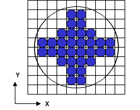
Fig. 8.1.35 The 10 \(\times\) 10 array of 32 uranium rods and 68 void cuboids with the array boundary.

The UNIT containing the ARRAY is now placed within the global unit using a HOLE content record. The location of the HOLE is determined using ORIGIN data to match the origin of the UNIT in the HOLE with an X, Y, Z position in the surrounding UNIT. In this problem, the origin of the UNIT must be at position (0,0,0). Since only nonzero data must be entered, ORIGIN data are not needed for this problem. The boundary region consists of the steel container.

GLOBAL UNIT 4
CYLINDER 2 4.6 6.37 -6.27
HOLE 3 ORIGIN X=0.0 Y=0.0 Z=0.0
MEDIA 2 1 2
BOUNDARY  2

The overall problem description is shown below. Two of the color plots used for verification of this mockup are shown in Fig. 8.1.36 and Fig. 8.1.37. The black outside border of the two color plots indicates volume outside the global unit. The plot can be extended just outside the global unit boundary to ensure that the entire problem is included in the plot. This results in a black area surrounding the actual problem.

KENO V.a:

=KENOVA
CASK ARRAY
READ PARAMETERS  FDN=YES LIB=41 GEN=10
END PARAMETERS
READ MIXT  SCT=1  MIX=1 92500 4.48006e-2  92800 2.6578e-3  92400 4.827e-4
92600 9.57e-5  MIX=2 100 1.0 END MIXT
READ GEOMETRY
UNIT 1
CYLINDER 1 1 0.5 2P5.0
CUBOID  0 1 4P0.5 2P5.0
UNIT 2
ARRAY 2 -1.0 -1.0 -5.0
GLOBAL UNIT 3
ARRAY  1 -2.0 -2.0 -5.0
CYLINDER 0 1 4.15 5.1 -5.0
HOLE 2 0.0 -3.0 0.0
HOLE 2 3.0 0.0 0.0
HOLE 2 0.0 3.0 0.0
HOLE 2 -3.0 0.0 0.0
CYLINDER 2 1 4.6 6.37 -6.27
END GEOM
READ ARRAY
ARA=1 NUX=4 NUY=4 NUZ=1 FILL F1 END FILL
ARA=2 NUX=2 NUY=2 NUZ=1 FILL F1 END FILL
END ARRAY
READ PLOT TTL='X-Z SLICE AT Y=0.25 WITH X ACROSS AND Z DOWN'
XUL=-5.0 YUL=0.25 ZUL=6.5 XLR=5.0 YLR=0.25 ZLR=-6.5
UAX=1.0 WDN=-1.0 NAX=640  END
TTL='X-Y SLICE AT Z=0.0 WITH X ACROSS AND Y DOWN'
XUL=-5.0 YUL=5.0 ZUL=0.0 XLR=5.0 YLR=-5.0 ZLR=0.0
UAX=1.0 VDN=-1.0 NAX=640 END
END PLOT
END DATA
END

KENO-VI:

KENO VI
CASK ARRAY
READ PARAMETERS  TME=1.0 FDN=YES LIB=41 GEN=10  END PARAMETERS
READ MIXT  SCT=1
MIX=1 92500 4.48006e-2  92800 2.6578e-3  92400 4.827e-4  92600 9.57e-5
MIX=2 100 1.0 END MIXT
READ GEOMETRY
UNIT 1
CYLINDER 1  0.5  2P5.0
CUBOID   2   4P0.5  2P5.0
MEDIA 1 1 1
MEDIA 0 1 2 -1
BOUNDARY  2
UNIT 2
CUBOID 1 4P0.5 2P5.0
MEDIA 0 1 1
BOUNDARY  1
UNIT 3
CYLINDER 1  4.15 5.0 -5.0
CYLINDER 2 4.15 5.1 -5.0
ARRAY 1 1 PLACE 5 5 1   -0.5 -0.5 -0.0
MEDIA 0 1 2 -1
BOUNDARY  2
GLOBAL UNIT 4
CYLINDER 2 4.6 6.37 -6.27
HOLE 3 ORIGIN X=0.0 Y=0.0 Z=0.0
MEDIA 2 1 2
BOUNDARY  2
END GEOM
READ ARRAY
ARA=1  NUX=10  NUY=10  NUZ=1  FILL  14*2 1 1 8*2 1 1 7*2 4*1 4*2 8*1 2 2 8*1 4*2 4*1 7*2 1 1
8*2 1 1 14*2  END FILL
END ARRAY
READ PLOT TTL='X-Z SLICE AT Y=0.25 WITH X ACROSS AND Z DOWN'
XUL=-5.0 YUL=0.25 ZUL=6.5 XLR=5.0 YLR=0.25 ZLR=-6.5
UAX=1.0 WDN=-1.0 NAX=640  END
TTL='X-Y SLICE AT Z=0.0 WITH X ACROSS AND Y DOWN'
XUL=-5.0 YUL=5.0 ZUL=0.0 XLR=5.0 YLR=-5.0 ZLR=0.0
UAX=1.0 VDN=-1.0 NAX=640 END
END PLOT
END DATA
END

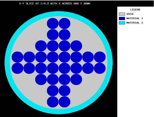
Fig. 8.1.36 X-Y slice of uranium rods in a cylindrical container.

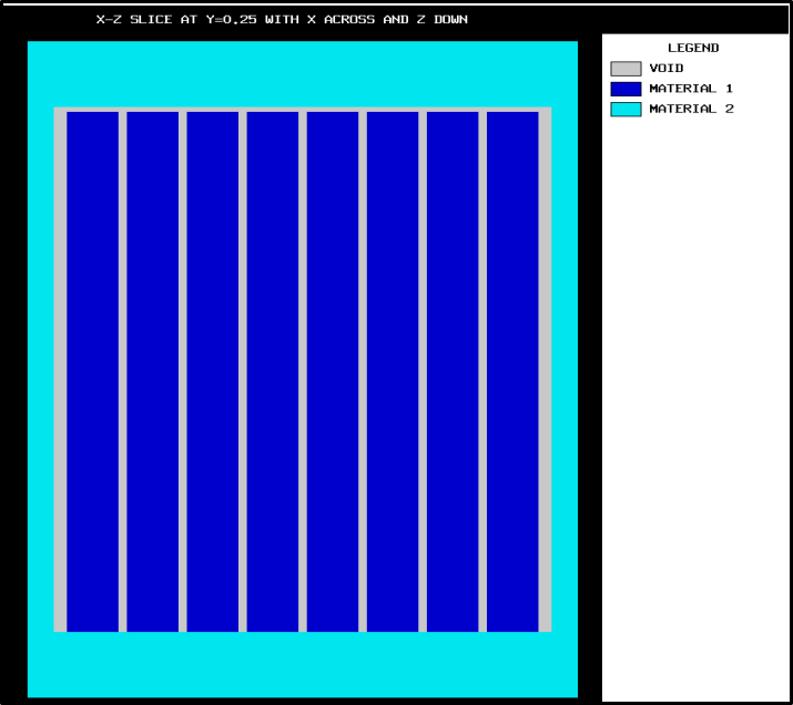
Fig. 8.1.37 X-Z slice of uranium rods in a cylindrical container.

EXAMPLE 20. A TYPICAL PRESSURIZED WATER REACTOR (PWR) SHIPPING CASK

A typical PWR shipping cask is illustrated in Fig. 8.1.38. The interior and exterior shell of the cask is carbon steel (mixture 7), and a depleted uranium gamma shield (mixture 6) is present in the annulus between the steel layers. The shipping cask contains seven PWR fuel assemblies. Each assembly is a 17 \(\times\) 17 ARRAY of fuel rods with water holes. Each assembly is contained in a stainless steel (mixture 5) box. Each fuel rod is composed of 4% enriched UO₂ (mixture 1) clad with Zircaloy (mixture 2). Rods of B₄C clad (mixture 4) with stainless steel are positioned between the fuel assemblies. The entire cask is filled with water (mixture 3).

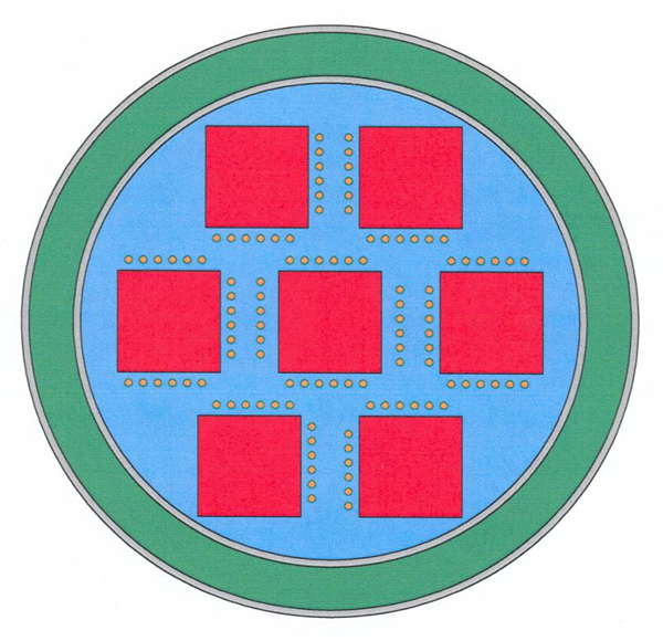
Fig. 8.1.38 Typical PWR shipping cask.

To describe the geometry of the cask, some simple units are defined as shown in Fig. 8.1.39. UNIT 1 represents a fuel rod and its associated square pitch spacing region. UNIT 2 represents a water hole in a fuel assembly. UNITs 3, 4, and 6 represent the B₄C rods with their various spacings, and UNIT 5 is a water hole that is used in association with some of the B₄C rods.

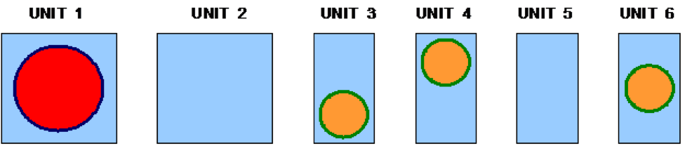
Fig. 8.1.39 Simple units.

KENO V.a:

UNIT 1
CYLINDER  1 1 .41148 365.76 0.0
CYLINDER  2 1 .48133 365.76 0.0
CUBOID    3 1 .63754 -.63754 .63754 -.63754 365.76 0.0

UNIT 2
CUBOID    3 1 .63754 -.63754 .63754 -.63754 365.76 0.0


UNIT 3
CYLINDER  4 1 .584 365.76 0.0
CYLINDER  5 1 .635 365.76 0.0
CUBOID    3 1 .9912 -.9912 2.2352 -1.27 365.76 0.0

UNIT 4
CYLINDER  4 1 .584 365.76 0.0
CYLINDER  5 1 .635 365.76 0.0
CUBOID    3 1 .9912 -.9912 1.2702 -2.235 365.76 0.0

UNIT 5
CUBOID    3 1 .9912 -.9912 1.7526 -1.7526 365.76 0.0

UNIT 6
CYLINDER  4 1 .584 365.76 0.0
CYLINDER  5 1 .635 365.76 0.0
CUBOID    3 1 1.1875215 -1.1875215 1.883706 -1.883706 365.76 0.0

KENO-VI:

UNIT 1
CYLINDER 1  .41148 365.76 0.0
CYLINDER 2  .48133 365.76 0.0
CUBOID   3  .63754 -.63754 .63754 -.63754 365.76 0.0
MEDIA 1 1 1
MEDIA 2 1 2 -1
MEDIA 3 1 3 -2
BOUNDARY  3

UNIT 2
CUBOID   1  .63754 -.63754 .63754 -.63754 365.76 0.0
MEDIA 3 1 1
BOUNDARY  1

UNIT 3
CYLINDER  1  .584 365.76 0.0
CYLINDER 2   .635 365.76 0.0
CUBOID    3   .9912 -.9912 2.2352 -1.27 365.76 0.0
MEDIA 4 1 1
MEDIA 5 1 2 -1
MEDIA 3 1 3 -2
BOUNDARY  3

UNIT 4
CYLINDER 1  .584 365.76 0.0
CYLINDER 2  .635 365.76 0.0
CUBOID   3   .9912 -.9912 1.2702 -2.235 365.76 0.0
MEDIA 4 1 1
MEDIA 5 1 2 -1
MEDIA 3 1 3 -2
BOUNDARY  3

UNIT 5
CUBOID 1   .9912 -.9912 1.7526 -1.7526 365.76 0.0
MEDIA 3 1 1
BOUNDARY  1

UNIT 6
CYLINDER 1  .584 365.76 0.0
CYLINDER 2  .635 365.76 0.0
CUBOID  3    1.1875215 -1.1875215 1.883706 -1.883706 365.76 0.0
MEDIA 4 1 1
MEDIA 5 1 2 -1
MEDIA 3 1 3 -2
BOUNDARY  3

UNITs 1 and 2 are stacked together into ARRAY 1 to form the ARRAY of fuel pins and water holes in a fuel assembly as shown in Fig. 8.1.40. This ARRAY is then encompassed with a layer of water and a layer of stainless steel to complete a fuel assembly in a storage cell (UNIT 7) as shown in Fig. 8.1.41.

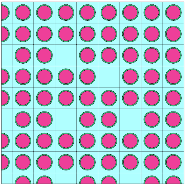
Fig. 8.1.40 Quarter section of fuel pin array.

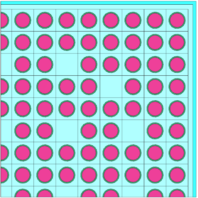
Fig. 8.1.41 Quarter section of fuel assembly.

KENO V.a:

ARA=1 NUX=17 NUY=17 NUZ=1 FILL
39R1 2 2Q3 8R1 2 9R1 2 22R1 2 4Q3 38R1 2 4Q3
Q51 22R1 2 Q10 Q9 2Q3 39R1                END FILL

UNIT 7
ARRAY 1 -10.83818 -10.83818 0.0
CUBOID    3 1 11.112495 -11.112495 11.112495 -11.112495 365.76 0.0
CUBOID    8 1 11.302238 -11.302238 11.302238 -11.302238 365.76 0.0

KENO-VI:

ARA=1 NUX=17 NUY=17 NUZ=1 FILL
39R1 2 2Q3 8R1 2 9R1 2 22R1 2 4Q3 38R1 2 4Q3
Q51 22R1 2 Q10 Q9 2Q3 39R1                END FILL
UNIT 7
CUBOID  1 10.83818 -10.83818 10.83818 -10.83818 365.76 0.0
CUBOID  2 11.112495 -11.112495 11.112495 -11.112495 365.76 0.0
CUBOID  3 11.302238 -11.302238 11.302238 -11.302238 365.76 0.0
ARRAY 1 1  PLACE 9 9 1  3*0.0
MEDIA 3 1 2 -1
MEDIA 5 1 3 -2
BOUNDARY  3

An array of UNIT 6s is created to represent the array of B₄C rods that is positioned between the fuel assemblies. In KENO V.a, the array of B₄C rods shown in Fig. 8.1.42 is contained in UNIT 8 for further use. KENO-VI geometry description does not need the placement of ARRAY 2 in a separate UNIT.

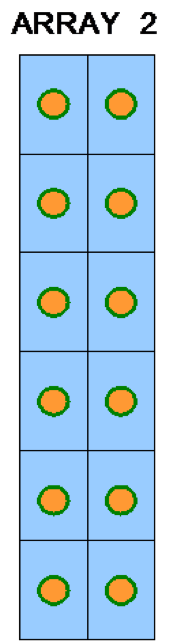
Fig. 8.1.42 2 \(\times\) 6 array of B₄C rods.

KENO V.a:

ARA=2 NUX=2 NUY=6 NUZ=1    FILL F6        END FILL

UNIT 8
ARRAY 2 0 0 0

KENO-VI:

ARA=2 NUX=2 NUY=6 NUZ=1    FILL F6        END FILL

The next step is to create the central array of three fuel assemblies with B₄C rods between them. In KENO V.a, this is done by stacking fuel assemblies in storage cells (UNIT 7) and B₄C rod arrays (UNIT 8) into an array (ARRAY 3) and placing it in a UNIT (UNIT 9). In KENO-VI description, UNIT 7 (fuel assembly in storage cell) and the array of B₄C rods (ARRAY 2) are directly placed into a UNIT (UNIT 8). The resultant geometry is shown in Fig. 8.1.43.

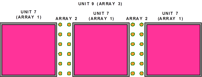
Fig. 8.1.43 Central array.

KENO V.a:

ARA=3 NUX=5 NUY=1 NUZ=1    FILL 7 8 7 8 7 END FILL

UNIT 9    ARRAY 3 0 0 0

KENO-VI:

UNIT 8
CUBOID 4  -11.302238 -16.052324 11.302238 -11.302238 365.76 0.0
CUBOID 5    16.052324 11.302238 11.302236 -11.302236 365.76 0.0
CUBOID 6    38.052324 -38.052324 11.302236 -11.302236 365.76 0.0
HOLE 7
HOLE 7 ORIGIN X= -27.354562
HOLE 7 ORIGIN X= 27.354562
ARRAY 2 4 PLACE 1 1 1 -14.8648025  -9.418530 0.0
ARRAY 2 5 PLACE 1 1 1  12.4897595  -9.418530 0.0
MEDIA 3 1 6 -5 -4
BOUNDARY  6

UNITs 3, 4, and 5 are used to define the arrays of B₄C rods that fit above and below the central array, as shown in Fig. 8.1.44.

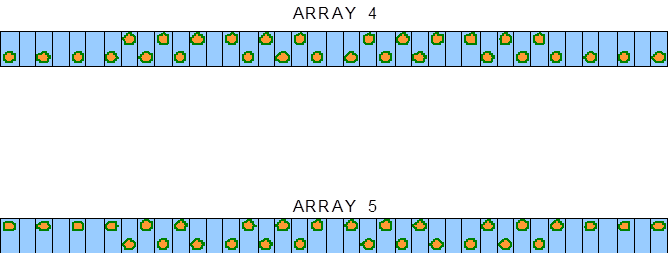
Fig. 8.1.44 Long B₄C rod arrays.

ARA=4 NUX=39 NUY=1 NUZ=1   FILL 3 5 2Q2 3 4 2Q2 5 4 3 2Q2 5 3 4 2Q2 5 4 3 2Q2 5 2Q2 3
END FILL

ARA=5 NUX=39 NUY=1 NUZ=1   FILL 4 5 2Q2 4 3 2Q2 5 3 4 2Q2 5 4 3 2Q2 5 3 4 2Q2 5 2Q2 4
END FILL

In KENO V.a these ARRAYs are placed in UNITs (UNITs 10 and 11) for further use.

KENO V.a:

UNIT 10   ARRAY 4 0 0 0

UNIT 11   ARRAY 5 0 0 0

UNITs 9, 10, and 11 in the KENO V.a description, or UNIT 8 and ARRAYs 3 and 4 in the KENO-VI description, are stacked to form the central array with B₄C rods as shown in Fig. 8.1.45.

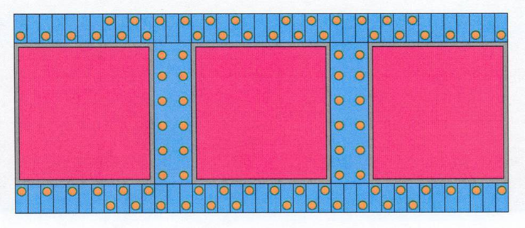
Fig. 8.1.45 Central array with long B₄C arrays.

KENO V.a:

ARA=6 NUX=1 NUY=3 NUZ=1    FILL 11 9  10  END FILL

KENO-VI:

CUBOID 2  38.052324 -38.052324 14.807436  11.302236  365.76 0.0
CUBOID 3  38.052324 -38.052324 11.302236 -14.807436  365.76 0.0
HOLE 8
ARRAY 3 2 PLACE 20 1 1 0.0 13.054836  0.0
ARRAY 4 3 PLACE 20 1 1 0.0 13.054836  0.0

This completes the three central fuel assemblies and all the B₄C rods associated with them. Next, UNITs 7 and 8 in KENO V.a geometry, UNIT 7 and ARRAY 2 in the KENO-VI geometry, are stacked together to form the array of two fuel assemblies separated by B₄C rods as shown in Fig. 8.1.46. This is designated as ARRAY 7 and UNIT 12 in KENO V.a, and UNIT 9 in KENO-VI. The origin of UNIT 12 for KENO V.a is specified at the center of the array in the X and Y directions and the bottom of the fuel assemblies (Z=27.94 cm). The origin of UNIT 9 in the KENO-VI description is specified at the center of the B₄C array in the X and Y directions and the bottom of the array in the Z direction.

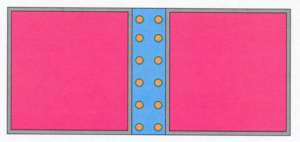
Fig. 8.1.46 Two fuel assemblies and B₄C rods.

KENO V.a:

ARA=7 NUX=3 NUY=1 NUZ=1    FILL 7 8 7     END FILL

UNIT 12   ARRAY 7 -24.979519 -11.302238 27.94

KENO-VI:

UNIT 9
CUBOID 1 2.375043 -2.375043  11.302236 -11.302236 365.76 0.0
CUBOID 4  24.979519  -23.7919975 11.302238 -11.302238 365.76 0.0
ARRAY 2 1 PLACE 1 1 1 -1.1875215 -9.418530 0.0
HOLE 7 ORIGIN X=-13.67728
HOLE 7 ORIGIN X=13.67728
MEDIA 0 1 4 -1
BOUNDARY  4

In KENO V.a, UNIT 13 is simply a cylindrical lid that fits on top of the shipping cask. It is described relative to the origin of the shipping cask and is made of depleted uranium.

KENO V.a:

UNIT 13
CYLINDER  6 1 47.625 457.2 449.58

All necessary subassemblies that make up the shipping cask have been built. The shipping cask is completed by specifying the origin of the central section (ARRAY 6 in KENO V.a) (see Fig. 8.1.45) to be at the center of the array in X and Y and the bottom of the array in the Z direction. A cylinder of water defining the interior of the shipping cask is described around the array. In the KENO V.a geometry, a HOLE is used to place UNIT 12 (Fig. 8.1.46) below the array, and a second HOLE is used to place another UNIT 12 above the array. In the KENO-VI geometry, UNIT 9 is placed as a HOLE above and below the central array. Then a cylinder of steel is placed around the water, which is in turn encased by depleted uranium. The depleted uranium is then contained in the outer steel cylinder of the shipping cask. In KENO V.a description, a third HOLE is used to place the depleted uranium lid (UNIT 13) on the shipping cask. This completes the shipping cask description of Fig. 8.1.38

The geometry data for this shipping cask are shown below. The plot data have been included for verification of the geometry description. However, the plot generated by this data is quite large and is therefore not included in this document.

KENO V.a:

READ GEOM
UNIT 1
CYLINDER  1 1 .41148 365.76 0.0
CYLINDER  2 1 .48133 365.76 0.0
CUBOID    3 1 .63754 -.63754 .63754 -.63754 365.76 0.0
UNIT 2
CUBOID    3 1 .63754 -.63754 .63754 -.63754 365.76 0.0
UNIT 3
CYLINDER  4 1 .584 365.76 0.0
CYLINDER  5 1 .635 365.76 0.0
CUBOID    3 1 .9912 -.9912 2.2352 -1.27 365.76 0.0
UNIT 4
CYLINDER  4 1 .584 365.76 0.0
CYLINDER  5 1 .635 365.76 0.0
CUBOID    3 1 .9912 -.9912 1.2702 -2.235 365.76 0.0
UNIT 5
CUBOID    3 1 .9912 -.9912 1.7526 -1.7526 365.76 0.0
UNIT 6
CYLINDER  4 1 .584 365.76 0.0
CYLINDER  5 1 .635 365.76 0.0
CUBOID    3 1 1.1875215 -1.1875215 1.883706 -1.883706 365.76 0.0
UNIT 7    ARRAY 1 -10.83818 -10.83818 0.0
CUBOID    3 1 11.112495 -11.112495 11.112495 -11.112495 365.76 0.0
CUBOID    8 1 11.302238 -11.302238 11.302238 -11.302238 365.76 0.0
UNIT 8    ARRAY 2 0 0 0
UNIT 9    ARRAY 3 0 0 0
UNIT 10   ARRAY 4 0 0 0
UNIT 11   ARRAY 5 0 0 0
UNIT 12   ARRAY 7 -24.979519 -11.302238 27.94
UNIT 13
CYLINDER  6 1 47.625 457.2 449.58
ARRAY     6  -38.6568 -14.807438 27.94
CYLINDER  3 1 47.625 447.04 16.51
HOLE     12    0.0 -26.1097 0.0
HOLE     12    0.0  26.1097 0.0
CYLINDER  7 1 48.895 447.04 13.335
CYLINDER  6 1 59.06 447.04 3.81
CYLINDER  7 1 63.01 462.28 0.0
HOLE     13    0.0 0.0 0.0
END GEOM
READ ARRAY
ARA=1 NUX=17 NUY=17 NUZ=1 FILL
39R1 2 2Q3 8R1 2 9R1 2 22R1 2 4Q3 38R1 2 4Q3
Q51 22R1 2 Q10 Q9 2Q3 39R1                END FILL
ARA=2 NUX=2 NUY=6 NUZ=1    FILL F6        END FILL
ARA=3 NUX=5 NUY=1 NUZ=1    FILL 7 8 7 8 7 END FILL
ARA=4 NUX=39 NUY=1 NUZ=1   FILL 3 5 2Q2 3 4 2Q2 5 4 3 2Q2 5 3 4 2Q2
5 4 3 2Q2 5 2Q2 3                         END FILL
ARA=5 NUX=39 NUY=1 NUZ=1   FILL 4 5 2Q2 4 3 2Q2 5 3 4 2Q2 5 4 3 2Q2
5 3 4 2Q2 5 2Q2 4                         END FILL
ARA=6 NUX=1 NUY=3 NUZ=1    FILL 11 9  10  END FILL
ARA=7 NUX=3 NUY=1 NUZ=1    FILL 7 8 7     END FILL
END ARRAY
READ PLOT
TTL=? SHIPPING CASK IF-300 X-Y SLICE  ?
XUL=-63 YUL=63 ZUL=180 XLR=63 YLR=-63 ZLR=180
UAX=1 VDN=-1 NAX=350
PLT=NO
END PLOT

KENO-VI:

READ GEOM
UNIT 1
CYLINDER  1 .41148 365.76 0.0
CYLINDER  2 .48133 365.76 0.0
CUBOID  3    .63754 -.63754 .63754 -.63754 365.76 0.0
MEDIA 1 1 1
MEDIA 2 1 2 -1
MEDIA 3 1 3 -2
BOUNDARY  3
UNIT 2
CUBOID  1  .63754 -.63754 .63754 -.63754 365.76 0.0
MEDIA 3 1 1
BOUNDARY  1
UNIT 3
CYLINDER 1   .584 365.76 0.0
CYLINDER 2   .635 365.76 0.0
CUBOID   3    .9912 -.9912 2.2352 -1.27 365.76 0.0
MEDIA 4 1 1
MEDIA 5 1 2 -1
MEDIA 3 1 3 -2
BOUNDARY  3
UNIT 4
CYLINDER 1  .584 365.76 0.0
CYLINDER 2  .635 365.76 0.0
CUBOID  3    .9912 -.9912 1.2702 -2.235 365.76 0.0
MEDIA 4 1 1
MEDIA 5 1 2 -1
MEDIA 3 1 3 -2
BOUNDARY  3
UNIT 5
CUBOID 1   .9912 -.9912 1.7526 -1.7526 365.76 0.0
MEDIA 3 1 1
BOUNDARY  1
UNIT 6
CYLINDER 1  .584 365.76 0.0
CYLINDER 2  .635 365.76 0.0
CUBOID  3    1.1875215 -1.1875215 1.883706 -1.883706 365.76 0.0
MEDIA 4 1 1
MEDIA 5 1 2 -1
MEDIA 3 1 3 -2
BOUNDARY  3
UNIT 7
CUBOID 1  10.83818 -10.83818 10.83818 -10.83818 365.76 0.0
CUBOID 2  11.112495 -11.112495 11.112495 -11.112495 365.76 0.0
CUBOID 3  11.302238 -11.302238 11.302238 -11.302238 365.76 0.0
ARRAY 1 1  PLACE 9 9 1  3*0.0
MEDIA 3 1 2 -1
MEDIA 8 1 3 -2
BOUNDARY  3
UNIT 8
CUBOID 4  -11.302238 -16.052324 11.302238 -11.302238 365.76 0.0
CUBOID 5    16.052324 11.302238 11.302236 -11.302236 365.76 0.0
CUBOID 6    38.052324 -38.052324 11.302236 -11.302236 365.76 0.0
HOLE 7
HOLE 7 ORIGIN X= -27.354562
HOLE 7 ORIGIN X= 27.354562
ARRAY 2 4 PLACE 1 1 1 -14.8648025  -9.418530 0.0
ARRAY 2 5 PLACE 1 1 1  12.4897595  -9.418530 0.0
MEDIA 0 1 6 -5 -4
BOUNDARY  6
UNIT 10
CUBOID 1 1.1875215 -1.1875215  11.302236 -11.302236 365.76 0.0
CUBOID 4  23.7919975 -23.7919975 11.302238 -11.302238 365.76 0.0
ARRAY 2 1 PLACE 1 1 1 3*0.0
HOLE 7 ORIGIN X=-12.4897595
HOLE 7 ORIGIN X=12.4897595
MEDIA 0 1 4 -1
BOUNDARY  4
GLOBAL UNIT 11
CUBOID 2  38.052324 -38.052324 13.284638  11.302236  365.76 0.0
CUBOID 3  38.052324 -38.052324 11.302236 -13.284638 365.76 0.0
CYLINDER 6 47.625 419.10  -11.43
CYLINDER 7   48.895 419.10 -14.605
CYLINDER 8  59.06 419.10 -24.13
CYLINDER 9  47.625 429.26 421.64
CYLINDER 10  63.01 434.34 -27.94
HOLE 8
ARRAY 3 2 PLACE 20 1 1 0.0 12.293438  0.0
ARRAY 4 3 PLACE 20 1 1 0.0 12.293438  0.0
HOLE 9 ORIGIN Y=24.586876
HOLE 9 ORIGIN Y=-24.586876
MEDIA 3 1 6 -3 -2
MEDIA 7 1 7 -6 -3 -2
MEDIA 6 1 8 -7
MEDIA 7 1 9
MEDIA 6 1 10 -9 -8
BOUNDARY  10
END GEOM
READ ARRAY
ARA=1 NUX=17 NUY=17 NUZ=1 FILL
39R1 2 2Q3 8R1 2 9R1 2 22R1 2 4Q3 38R1 2 4Q3
Q51 22R1 2 Q10 Q9 2Q3 39R1                END FILL
ARA=2 NUX=2 NUY=6 NUZ=1    FILL F6        END FILL
ARA=3 NUX=5 NUY=1 NUZ=1    FILL 7 8 7 8 7 END FILL
ARA=4 NUX=39 NUY=1 NUZ=1   FILL 3 5 2Q2 3 4 2Q2 5 4 3 2Q2 5 3 4 2Q2
5 4 3 2Q2 5 2Q2 3                         END FILL
ARA=5 NUX=39 NUY=1 NUZ=1   FILL 4 5 2Q2 4 3 2Q2 5 3 4 2Q2 5 4 3 2Q2
5 3 4 2Q2 5 2Q2 4                         END FILL
ARA=6 NUX=1 NUY=3 NUZ=1    FILL 11 9  10  END FILL
ARA=7 NUX=3 NUY=1 NUZ=1    FILL 7 8 7     END FILL
END ARRAY
READ PLOT
TTL=? SHIPPING CASK IF-300 X-Y SLICE  ?
XUL=-63 YUL=63 ZUL=180 XLR=63 YLR=-63 ZLR=180
UAX=1 VDN=-1 NAX=350
PLT=NO
END PLOT

8.1.4.6.5. Triangular pitched arrays in KENO-VI

EXAMPLE 21.

Triangular pitched ARRAYs can be described in KENO-VI by defining the UNITs that make up the ARRAY as HEXPRISM and in the array data block setting TYP=TRIANGULAR, HEXAGONAL, SHEXAGONAL, or RHEXAGONAL. This includes close-packed triangular pitched arrays. Since the ARRAYs are constructed by stacking hexprisms, care must be taken to ensure that the ARRAY boundary is completely enclosed within the stacked UNIT. Below is an example of a triangular pitched ARRAY.

The first and second UNITs are the HEXPRISMs that make up the ARRAY. UNIT 1 is the fuel cell stacked in a triangular pitched or hexagonal lattice. UNIT 2 is a dummy UNIT used to fill in the ARRAY so the array boundary is contained within the stacked UNITs. Since the ARRAY is not moderated, UNIT 2 contains void. Fig. 8.1.47 shows an X-Y cross section schematic of UNITs 1 and 2.

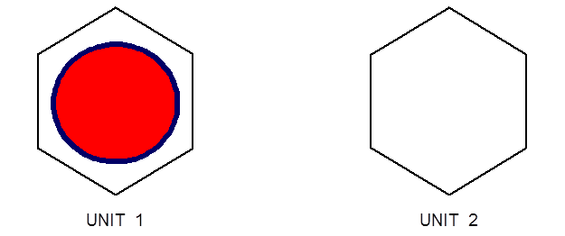
Fig. 8.1.47 Fuel cell and empty cell set up as hexprisms.

UNIT  1
COM='SINGLE CELL FUEL CAN IN HEXPRISM'
CYLINDER 10  10.16  18.288  0.0
CYLINDER 20  10.312 18.288 -0.152
HEXPRISM 30  10.503 18.288 -0.152
MEDIA  1  1  10
MEDIA  2  1  20  -10
MEDIA  0  1  30  -20
BOUNDARY  30
UNIT  2
COM='EMPTY CELL'
HEXPRISM  10  10.503  18.288  -0.152
MEDIA  0  1  10
BOUNDARY  10

UNIT 3 is the GLOBAL UNIT that contains the ARRAY and ARRAY BOUNDARY. The ARRAY is an unmoderated triangular pitched assembly of 7 cells. Unrotated triangular or hexagonal pitched arrays can be set up in two array configurations. The first configuration, selected using the TYP= followed by keyword HEXAGONAL or TRIANGULAR, stacks the UNITs so that the faces perpendicular to the X axis meet. Each consecutive row in the Y direction begins \(1/2\) of the face-to-face dimension farther over in the positive X direction than in the previous row. The second configuration, selected using the TYP= followed by keyword SHEXAGONAL, also stacks the UNITs so that the faces perpendicular to the X axis meet. However, for this type of ARRAY, the odd numbered rows in the Y direction (1, 3, 5, etc.) begin at the left edge of the ARRAY, and the even numbered rows in the Y direction (2, 4, 6, etc.) begin \(1/2\) of the face-to-face dimension to the right of the left edge of the ARRAY. Fig. 8.1.48 and Fig. 8.1.49 show X-Y cross section schematics of the assembly for the two different unrotated hexagonal ARRAY types.

GLOBAL UNIT 3
COM='7 CYLINDERS IN A CIRCLE WITH CYLINDRICAL BOUNDARY'
CYLINDER 10  32.000  18.288  -0.152
ARRAY  1  10 PLACE 3 3 1 3*0.0
BOUNDARY 10
READ ARRAY GBL=1 ARA=1 TYP=HEXAGONAL NUX=5 NUY=5 NUZ=1
FILL 7*2 2*1 2*2 3*1 2*2 2*1 7*2 END FILL  END ARRAY

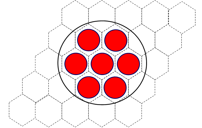
Fig. 8.1.48 Seven cylinders stacked in a HEXAGONAL array with cylindrical array boundary.

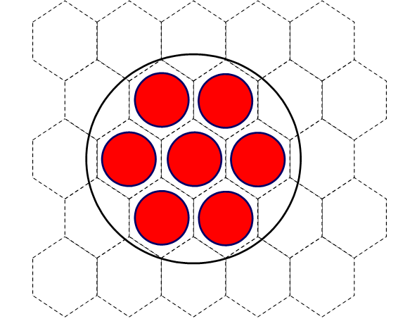
Fig. 8.1.49 Seven cylinders stacked in a SHEXAGONAL array with a cylindrical array boundary.

The overall problem description is shown below. The cross section library would be generated in a separate CSAS-MG step. An X-Y cross section color plot used for verification of this mockup is shown in Fig. 8.1.50.

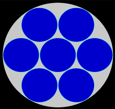
Fig. 8.1.50 X-Y slice of 7 cylinders in a triangular pitch array.

Data description of Example 21.

=KENOVI
TRIANGULAR PITCHED ARRAY 7 PINS IN A CIRCLE
READ PARAMETERS LNG=20000 LIB=4 END PARAMETERS
READ MIXT SCT=2
MIX=1 NCM=8 92235 1.37751E-03  92238 9.92354E-05  8016 3.32049E-02
       9019 2.95349E-03  1001 6.05028E-02
MIX=2 NCM=14 13027 6.02374E-02
END MIXT
READ GEOMETRY
UNIT 1
COM='SINGLE CELL FUEL CAN IN HEXPRISM'
CYLINDER 10  10.16  18.288  0.0
CYLINDER 20  10.312 18.288 -0.152
HEXPRISM 30  10.503 18.288 -0.152
MEDIA  1 1 10
MEDIA  2 1 20 -10
MEDIA 0 1 30 -20
BOUNDARY  30
UNIT 2
COM='EMPTY CELL'
HEXPRISM 10  10.503 18.288 -0.152
MEDIA  0 1 10
BOUNDARY  10
GLOBAL UNIT 3
CYLINDER 10  32.000 18.288 -0.152
COM='7 CYLINDERS IN A CIRCLE WITH CYLINDRICAL BOUNDARY'
ARRAY  1 10 PLACE 3 3 1 3*0.0
BOUNDARY  10
END GEOMETRY
READ ARRAY  GBL=1 TYP=HEXAGONAL NUX=5 NUY=5 NUZ=1
FILL 7*2 2*1 2*2 3*1 2*2 2*1 7*2 END FILL  END ARRAY
READ PLOT
TTL='TRIANGULAR PITCHED ARRAY, 7 PINS IN A CIRCLE'
XUL=-33.0  YUL=33.0  ZUL=0.0
XLR=33.0  YLR=-33.0  ZLR=0.0
UAX=1  VDN=-1  NAX=640    END
END PLOT
END DATA
END

EXAMPLE 21a.

Another hexagonal ARRAY type involves stacking rotated hexprisms, which are hexprisms rotated 30\(^{\circ}\)/ 90\(^{\circ}\) so that the flat faces perpendicular to the Y axis now meet. Rotated hexagonal arrays are specified by setting TYP=RHEXAGONAL in the array data block. Because the ARRAYs are constructed by stacking hexprisms, care must be taken to ensure the array boundary is completely enclosed within the stacked UNIT. Below is an example of a rotated hexagonal pitched ARRAY.

The first and second UNITs are the rotated hexprisms that make up the ARRAY. They are specified using the geometry keyword RHEXPRISM. UNIT 1 is the fuel cell that is stacked in a rotated hexagonal lattice. UNIT 2 is a dummy UNIT used to fill in the ARRAY so that the ARRAY BOUNDARY is contained within the stacked UNITs. Since the ARRAY is not moderated, UNIT 2 contains void. Fig. 8.1.51 shows an X-Y cross section schematic of UNITs 1 and 2.

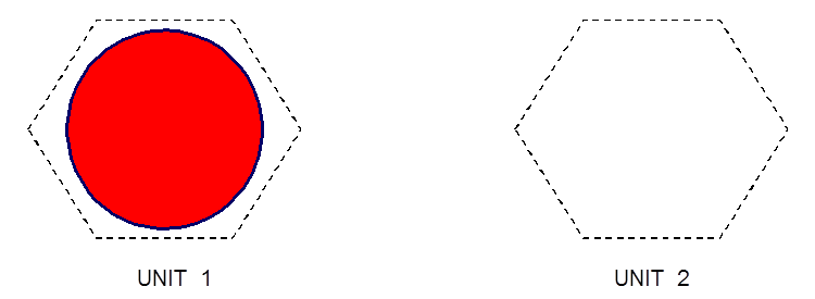
Fig. 8.1.51 Fuel cell and empty cell set up as rotated hexprism (RHEXPRISM).

UNIT  1
COM='SINGLE CELL FUEL CAN IN HEXPRISM'
CYLINDER 10  10.16  18.288  0.0
CYLINDER 20  10.312 18.288 -0.152
RHEXPRISM 30  10.503 18.288 -0.152
MEDIA  1  1  10
MEDIA  2  1  20  -10
MEDIA  0  1  30  -20
BOUNDARY  30
UNIT  2
COM='EMPTY CELL'
RHEXPRISM  10  10.503  18.288  -0.152
MEDIA  0  1  10
BOUNDARY  10

UNIT 3 is the GLOBAL UNIT that contains the ARRAY and ARRAY BOUNDARY. The ARRAY is an unmoderated rotated hexagonal pitched assembly of 7 cells. The rotated hexagonal array type is specified in the array data block using TYP= with the keyword RHEXAGONAL. This ARRAY type stacks the UNITs so the faces perpendicular to the Y axis meet. In the odd numbered columns (i.e., 1, 3, 5, etc.), the UNITs are stacked so the columns begin at the lower edge of the array and in the even numbered columns (i.e., 2, 4, 6, etc.), the UNITs are stacked so the columns begin \(1/2\) of the face-to-face dimension above the lower edge of the ARRAY. Fig. 8.1.52 shows the X-Y cross section schematic of the assembly for the rotated hexagonal ARRAY type.

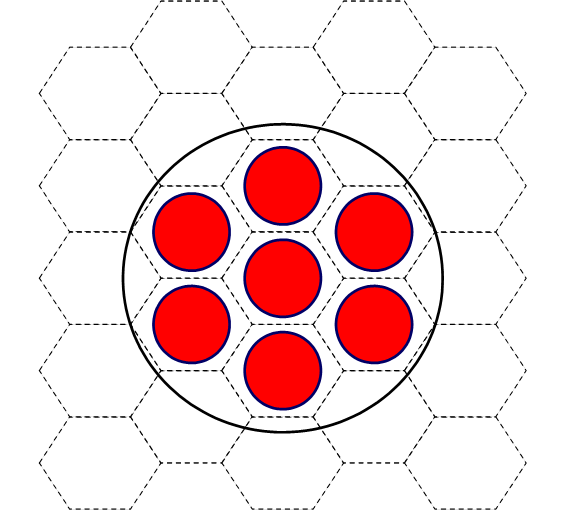
Fig. 8.1.52 Seven cylinders stacked in a RHEXAGONAL array with a cylindrical array boundary.

GLOBAL UNIT 3
COM='7 CYLINDERS IN A CIRCLE WITH CYLINDRICAL BOUNDARY'
CYLINDER 10  32.000  18.288  -0.152
ARRAY  1  10 PLACE 3 3 1 3*0.0
BOUNDARY 10
READ ARRAY GBL=1 ARA=1 TYP=RHEXAGONAL NUX=5 NUY=5 NUZ=1
FILL 6*2 3*1 2*2 3*1 3*2 1*1 7*2 END FILL  END ARRAY

The overall problem description is shown below. The cross section library would be generated in a separate CSAS-MG step. An X-Y cross section color plot used for verification of this mockup is shown in Fig. 8.1.53.

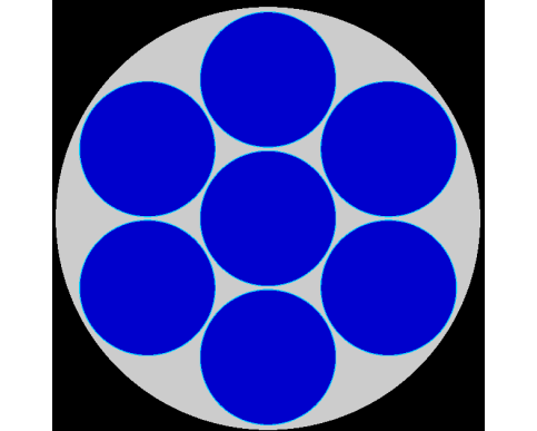
Fig. 8.1.53 X-Y slice of 7 cylinders in a rotated hexagonal pitched array.

Data description of Example 21a.

=KENOVI
TRIANGULAR PITCHED ARRAY 7 PINS IN A CIRCLE
READ PARAMETERS LNG=20000 LIB=4 END PARAMETERS
READ MIXT SCT=2
MIX=1 NCM=8 92235 1.37751E-03  92238 9.92354E-05  8016 3.32049E-02
       9019 2.95349E-03  1001 6.05028E-02
MIX=2 NCM=14 13027 6.02374E-02
END MIXT
READ GEOMETRY
UNIT 1
COM='SINGLE CELL FUEL CAN IN HEXPRISM'
CYLINDER 10  10.16  18.288  0.0
CYLINDER 20  10.312 18.288 -0.152
RHEXPRISM 30  10.503 18.288 -0.152
MEDIA  1 1 10
MEDIA  2 1 20 -10
MEDIA 0 1 30 -20
BOUNDARY  30
UNIT 2
COM='EMPTY CELL'
RHEXPRISM 10  10.503 18.288 -0.152
MEDIA  0 1 10
BOUNDARY  10
GLOBAL UNIT 3
CYLINDER 10  32.000 18.288 -0.152
COM='7 CYLINDERS IN A CIRCLE WITH CYLINDRICAL BOUNDARY'
ARRAY  1 10 PLACE 3 3 1 3*0.0
BOUNDARY  10
END GEOMETRY
READ ARRAY  GBL=1 TYP=RHEXAGONAL NUX=5 NUY=5 NUZ=1
FILL 6*2 3*1 2*2 3*1 3*2 1*1 7*2 END FILL  END ARRAY
READ PLOT
TTL='ROTATED HEXAGONAL ARRAY, 7 PINS IN A CIRCLE'
XUL=-33.0  YUL=33.0  ZUL=0.0
XLR=33.0  YLR=-33.0  ZLR=0.0
UAX=1  VDN==-1  NAX=640    END
END PLOT
END DATA
END

8.1.4.6.6. Triangular pitched Arrays in KENO V.a

Triangular pitched arrays can be described in KENO V.a geometry by properly defining the basic unit from which the array can be built. This includes close-packed triangular pitched arrays. Two geometry configurations are described below.

EXAMPLE 1. Bare Triangular pitched Array.

Fig. 8.1.54 illustrates a small close-packed triangular pitched ARRAY. Each rod in the ARRAY has a radius of 2.0 cm, and the pitch of the ARRAY is 4 cm. To create this ARRAY, describe five units as defined in Fig. 8.1.55.

Assume the rods described in the ARRAY are each 2.0 cm in radius and 100 cm tall. The rods are composed of mixture 1. The geometry descriptions for the first four UNITs are given below.

UNIT 1
ZHEMICYL-Y 1 1 2.0 50.0 -50.0

UNIT 2
ZHEMICYL+Y 1 1 2.0 50.0 -50.0

UNIT 3
ZHEMICYL-X 1 1 2.0 50.0 -50.0

UNIT 4
ZHEMICYL+X 1 1 2.0 50.0 -50.0

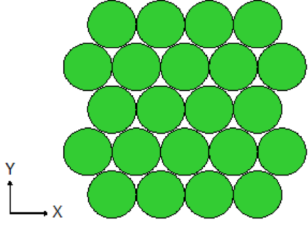
Fig. 8.1.54 Bare triangular pitched ARRAY.

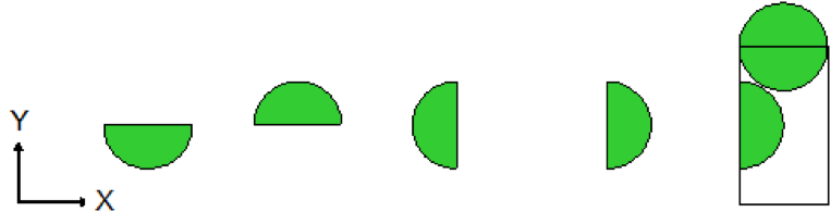
Fig. 8.1.55 Units used to describe a bare triangular pitched ARRAY.

To describe UNIT 5, the origin of the UNIT is defined to be at its center. One of the hemicylinders is built into the box, and the other three are added as holes. In this example, the +X hemicylinder is built into the box, and the other hemicylinders are inserted as holes. (Because the +X hemicylinder is built into UNIT 5, UNIT 4 is not used in the problem.) The half dimension of the box in the X dimension is equal to the radius, 2.0 cm. The half dimension of the box in the Y direction is \(\frac{\sqrt{3}}{2}\) times the pitch (0.866025 * 4.0) or 3.46411 cm. UNIT 5 is described below.

UNIT 5
ZHEMICYL+X  1 1 2.0 50.0 -50.0 ORIGIN -2.0 0.0
CUBOID  0 1 2P2.0 2P3.46411 2P50.0
HOLE 1 0.0  3.46411   0.0
HOLE 2 0.0 -3.46411   0.0
HOLE 3 2.0            0.0

In the description of UNIT 5, the ZHEMICYL+X places the hemicylinder at the left of the box. HOLE 1 places the top hemicylinder, HOLE 2 places the bottom hemicylinder, and HOLE 3 places the hemicylinder at the right of the box.

Next, a UNIT 6 is defined that can be used to complete the lower rod of UNIT 5. A UNIT 7 is defined that can be used to complete the upper rod of UNIT 5. UNIT 8 is defined to complete the left rod of UNIT 5, and UNIT 9 is defined to complete the right rod of UNIT 5. UNIT 10 is defined to complete the corners of the overall ARRAY. The input data for these UNITs are given below and are illustrated in Fig. 8.1.56.

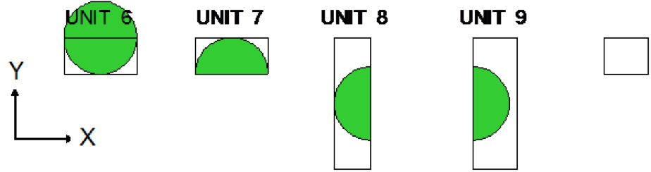
Fig. 8.1.56 UNITs to complete the triangular pitched ARRAY.

UNIT 6
ZHEMICYL-Y       1 1 2.0 50.0 -50.0
CUBOID           0 1 2P2.0 0.0 -2.0 50.0 -50.0

UNIT 7
ZHEMICYL+Y   1 1 2.0 50.0 -50.0
CUBOID           0 1 2P2.0 2.0 0.0 2P50.0

UNIT 8
ZHEMICYL-X       1 1 2.0 50.0 -50.0
CUBOID           0 1 0.0 -2.0 2P3.46411 2P50.0

UNIT 9
ZHEMICYL+X   1 1 2.0 50.0 -50.0
CUBOID           0 1 2.0 0.0 2P3.46411 2P50.0

UNIT 10
CUBOID           0 1 2.0 0.0 2.0 0.0 2P50.0

Fig. 8.1.57 shows the arrangement of the UNITs to complete the ARRAY. The data to describe the ARRAY are shown below.

ARA=1 NUX=6 NUY=4 NUZ=1
FILL 10 4R6 10 8 4R5 9 1Q6 10 4R7 10 END FILL

The bottom row of the ARRAY is described by the data entries 10 4R6 10. The second row of the ARRAY is described by the data entries 8 4R5 9. The third row is filled by repeating the previous six entries (1Q6). It could also have been described by entering 8 4R5 9. The top row of the ARRAY is described by the data entries 10 4R7 10.

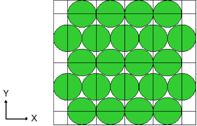
Fig. 8.1.57 Completed ARRAY.

EXAMPLE 2a. Triangular Pitched ARRAY in a Cylinder

Fig. 8.1.58 illustrates a close-packed triangular pitched ARRAY in a cylinder. This array may be described by defining five basic units that are the same as those of Example 1 shown in Fig. 8.1.55.

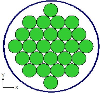
Fig. 8.1.58 Triangular pitched ARRAY within a cylinder.

UNIT 1
ZHEMICYL-Y 1 1 2.0 50.0 -50.0

UNIT 2
ZHEMICYL+Y 1 1 2.0 50.0 -50.0

UNIT 3
ZHEMICYL-X 1 1 2.0 50.0 -50.0

UNIT 4
ZHEMICYL+X 1 1 2.0 50.0 -50.0

To describe UNIT 5, the origin of the UNIT to be at its center is defined. One of the hemicylinders is built into the box, and the other three are added as HOLEs. In this example, the +X hemicylinder is built into the box, and the other hemicylinders are inserted as HOLEs. The half dimension of the box in the X dimension is equal to the radius, 2.0 cm. The half dimension of the box in the Y direction is \(\frac{\sqrt{3}}{2}\) times the pitch (0.866025 * 4.0) or 3.46411 cm. UNIT 5 is described below.

UNIT 5
ZHEMICYL+X 1 1 2.0 50.0 -50.0 ORIGIN -2.0 0.0
CUBOID     0 1 2P2.0 2P3.46411 2P50.0
HOLE 1  0.0  3.46411 0.0
HOLE 2  0.0 -3.46411 0.0
HOLE 3  2.0  0.0     0.0

In the description of UNIT 5, the ZHEMICYL+X places the hemicylinder at the left of the box. HOLE 1 places the top hemicylinder, HOLE 2 places the bottom hemicylinder, and HOLE 3 places the hemicylinder at the right of the box.

To describe the base ARRAY of the problem, UNITs 5 is stacked in a 4 \(\times\) 2 \(\times\) 1 array as shown in Fig. 8.1.59. The input data for the ARRAY are the following:

ARA=1 NUX=4 NUY=2 NUZ=1  FILL F5 END FILL

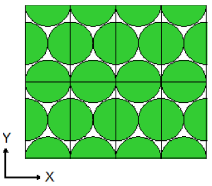
Fig. 8.1.59 4 \(\times\) 2 \(\times\) 1 array to be placed within a cylinder.

Next, the ARRAY is placed within the cylinder. This is done by placing the ARRAY in a UNIT, defined here to be UNIT 6. The origin of the cylinder has been defined to be at the center of the ARRAY. The resulting geometry is shown in Fig. 8.1.60.

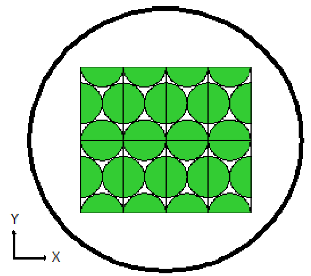
Fig. 8.1.60 4 \(\times\) 2 \(\times\) 1 ARRAY within a cylinder.

UNIT 6
ARRAY 1 -8.0 -6.92822 -50.0
CYLINDER 0 1 12.4  2P50.0
CYLINDER 2 1 12.65 2P50.0

Next, the hemicylinders necessary to complete all of the half cylinders remaining in Fig. 8.1.60 are added. This is done by placing four UNITs 1 at the appropriate positions along the bottom of the ARRAY, four UNITs 2 at the top of the ARRAY, two UNITs 3 at the left of the ARRAY, and two UNITs 4 at the right of the ARRAY. The input data are shown below, and the resulting configuration is shown in Fig. 8.1.61. In UNIT 6, the first HOLE 1 places a UNIT 1 under the lower left UNIT of the ARRAY. The second HOLE 1 places a UNIT 1 under the next ARRAY UNIT to the right of the first one. This procedure is repeated for the next two lower ARRAY UNITs, thus completing the lower row of cylinders. Similarly, the first HOLE 2 places a UNIT 2 above the upper left UNIT of the ARRAY. The second HOLE 2 places a UNIT 1 to the right of the first one, etc., until the four cylinders at the top of the ARRAY are completed. The first HOLE 3 places a UNIT 3 at the lower left side of the ARRAY to complete that rod. The second HOLE 3 completes the rod above it. The first HOLE 4 completes the lower rod on the right side of the ARRAY. The second HOLE 4 completes the rod above it. The geometry data listed below result in the configuration shown in Fig. 8.1.61.

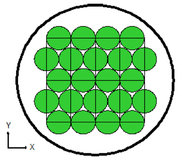
Fig. 8.1.61 Partially completed triangular pitched ARRAY in a cylinder.

UNIT 6
ARRAY 1 -8.0 -6.92822 -50.0
CYLINDER 0 1 12.4  2P50.0
HOLE 1  -6.0 -6.92822 0.0
HOLE 1  -2.0 -6.92822 0.0
HOLE 1   2.0 -6.92822 0.0
HOLE 1   6.0 -6.92822 0.0
HOLE 2  -6.0  6.92822 0.0
HOLE 2  -2.0  6.92822 0.0
HOLE 2   2.0  6.92822 0.0
HOLE 2   6.0  6.92822 0.0
HOLE 3  -8.0 -3.46411 0.0
HOLE 3  -8.0  3.46411 0.0
HOLE 4   8.0 -3.46411 0.0
HOLE 4   8.0  3.46411 0.0
CYLINDER 2 1 12.65 2P50.0

To complete the desired configuration, a cylinder is defined, UNIT 7, and it is placed at the four appropriate positions as shown below. The first HOLE 7 places the cylinder of UNIT 7 at the left of the ARRAY, the second HOLE 7 places the cylinder at the top of the ARRAY, the third HOLE 7 places the cylinder at the right of the ARRAY, and the fourth HOLE 7 places the cylinder at the bottom of the ARRAY. The completed configuration is shown in Fig. 8.1.62. It is not necessary for UNIT 7 to precede UNIT 6. It is allowable to place UNIT 7 after UNIT 6 in the input data. Because the final configuration is defined in UNIT 6, it must be designated as the GLOBAL UNIT. The total geometry input for this example is listed below.

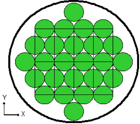
Fig. 8.1.62 Completed triangular pitched array in a cylinder.

READ GEOM
UNIT 1
ZHEMICYL-Y 1 1 2.0 50.0 -50.0

UNIT 2
ZHEMICYL+Y 1 1 2.0 50.0 -50.0

UNIT 3
ZHEMICYL-X 1 1 2.0 50.0 -50.0

UNIT 4
ZHEMICYL+X 1 1 2.0 50.0 -50.0

UNIT 5
ZHEMICYL+X 1 1 2.0 50.0 -50.0 ORIGIN -2.0 0.0
CUBOID     0 1 2P2.0 2P3.46411 2P50.0
HOLE 1  0.0  3.46411 0.0
HOLE 2  0.0 -3.46411 0.0
HOLE 3  2.0  0.0     0.0

UNIT 7
CYLINDER 1 1 2.0 2P50.0

GLOBAL UNIT 6
ARRAY 1 -8.0 -6.92822 -50.0
CYLINDER 0 1  12.4  2P50.0
HOLE 1  -6.0  -6.92822 0.0
HOLE 1  -2.0  -6.92822 0.0
HOLE 1   2.0  -6.92822 0.0
HOLE 1   6.0  -6.92822 0.0
HOLE 2  -6.0   6.92822 0.0
HOLE 2  -2.0   6.92822 0.0
HOLE 2   2.0   6.92822 0.0
HOLE 2   6.0   6.92822 0.0
HOLE 3  -8.0  -3.46411 0.0
HOLE 3  -8.0   3.46411 0.0
HOLE 4   8.0  -3.46411 0.0
HOLE 4   8.0   3.46411 0.0
HOLE 7 -10.0   0.0     0.0
HOLE 7   0.0  10.39233 0.0
HOLE 7  10.0   0.0     0.0
HOLE 7   0.0 -10.39233 0.0
CYLINDER 2 1  12.65 2P50.0
END GEOM

READ ARRAY
ARA=1 NUX=4 NUY=2 NUZ=1  FILL F5 END FILL
END ARRAY

EXAMPLE 2b. Alternative Mockup of Triangular Pitched ARRAY in a Cylinder.

Consider the triangular pitched ARRAY shown in Fig. 8.1.58. Another method of describing this configuration is given below. Four basic UNITs are defined, as listed below. These are the same UNITs shown in Fig. 8.1.55.

UNIT 1
ZHEMICYL-Y 1 1 2.0 50.0 -50.0

UNIT 2
ZHEMICYL+Y 1 1 2.0 50.0 -50.0

UNIT 3
ZHEMICYL-X 1 1 2.0 50.0 -50.0

UNIT 4
ZHEMICYL+X 1 1 2.0 50.0 -50.0

UNIT 5 is the same as previously defined in Example 2a, and pictured in Fig. 8.1.55.

UNIT 5
ZHEMICYL+X 1 1 2.0 50.0 -50.0 ORIGIN -2.0 0.0
CUBOID     0 1 2P2.0 2P3.46411 2P50.0
HOLE 1  0.0  3.46411 0.0
HOLE 2  0.0 -3.46411 0.0
HOLE 3  2.0  0.0     0.0

To describe the basic array for the problem, UNITs 5 is stacked in a 4 \(\times\) 2 \(\times\) 1 as shown in Fig. 8.1.59. The input data for the ARRAY are the following:

ARA=1 NUX=4 NUY=2 NUZ=1  FILL F5 END FILL

Next, the ARRAY (ARRAY 1) is placed in UNIT 6, and UNITs 7 and 8 are defined to be placed to the left and right of it (see Fig. 8.1.63). UNIT 7 will complete the two rods at the left boundary of the ARRAY and will contain half of the far left rod in the completed configuration. In the description of UNIT 7, the ZHEMICYL+X is half of the far right rod and is located with its cut face at the left boundary of a box that is as tall as the entire ARRAY of Fig. 8.1.59. The first HOLE 3 in UNIT 7 completes the lower left rod of that ARRAY, and the second HOLE 3 completes the upper left rod. UNIT 8 is constructed in similar fashion to complete the two rods at the right of the ARRAY shown in Fig. 8.1.59. UNIT 8 is the mirror image of UNIT 7. UNITs 6, 7, and 8 are stacked in an ARRAY (ARRAY2) to achieve the configuration shown in Fig. 8.1.63. The data to accomplish this are listed below.

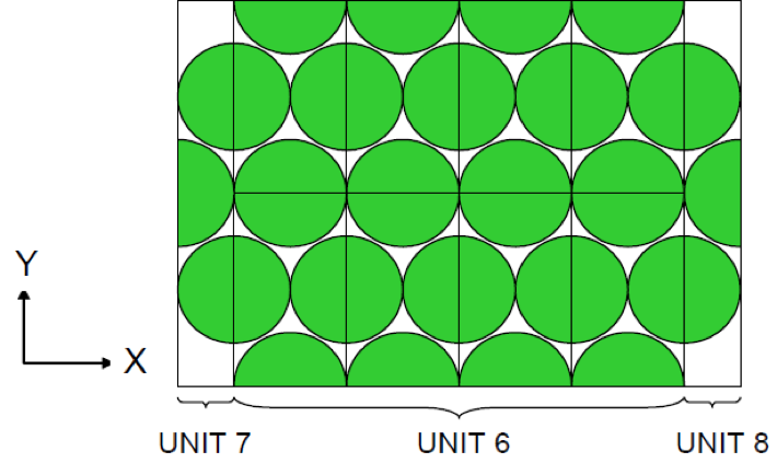
Fig. 8.1.63 Array to be placed in a cylinder.

UNIT 6
ARRAY 1 -8.0 -6.92822 -50.0

GLOBAL
UNIT 7
ZHEMICYL+X 1 1 2.0 50.0 -50.0
CUBOID     0 1 2.0 0.0 2P6.92822 2P50.0
HOLE 3 2.0 -3.46411 0.0
HOLE 3 2.0  3.46411 0.0

UNIT 8
ZHEMICYL-X 1 1 2.0 50.0 -50.0
CUBOID     0 1 0.0 -2.0 2P6.92822 2P50.0
HOLE 4 -2.0 -3.46411 0.0
HOLE 4 -2.0  3.46411 0.0

ARA=2 NUX=3 NUY=1 NUZ=1 FILL 7 6 8 END FILL

Next, ARRAY 2 is placed in the cylinder as shown in Fig. 8.1.64. The data are listed below.

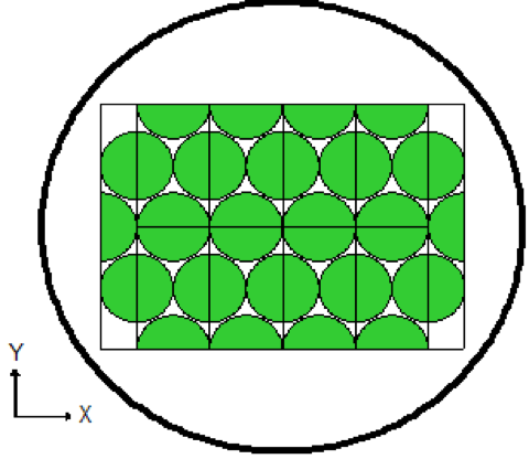
Fig. 8.1.64 Partially completed array in a cylinder.

UNIT 9
ARRAY 2 -10.0 -6.92822 -50.0
CYLINDER 0 1 12.4  2P50.0
CYLINDER 2 1 12.65 2P50.0

Now UNITs 10 and 11 are described and placed above and below the ARRAY. These UNITs are shown in Fig. 8.1.65. UNIT 10 is described to complete the two central rods at the top of the ARRAY of Fig. 8.1.64. Fig. 8.1.65 and Fig. 8.1.66 illustrate these UNITs. The ZHEMICYL-Y is placed at the top of the UNIT to describe half of the rod at the very top of the ARRAY. The first HOLE 2 completes the left center rod at the top of the ARRAY pictured in Fig. 8.1.64. The second HOLE 2 completes the right center rod at the top of the ARRAY. UNIT 11 is described in similar fashion. It is the mirror image of UNIT 10 and is placed below the ARRAY of Fig. 8.1.64. The resulting configuration is shown in Fig. 8.1.65.

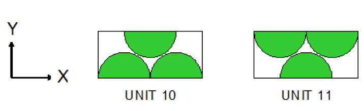
Fig. 8.1.65 Description of UNITs 10 and 11 for Example 2b.

UNIT 10
ZHEMICYL-Y 1 1 2.0 2P50.0
CUBOID  0 1 2P4.0 0.0 -3.46411 2P50.0
HOLE 2 -2.0 -3.46411 0.0 2P50.0
HOLE 2  2.0 -3.46411 0.0

UNIT 11
ZHEMICYL+Y 1 1 2.0 2P50.0
CUBOID  0 1 2P4.0 3.46411 0.0 2P50.0
HOLE 1 -2.0 3.46411 0.0
HOLE 1  2.0 3.46411 0.0

Now UNITs 10 and 11 are placed above and below the ARRAY of Fig. 8.1.64 to obtain the configuration shown in Fig. 8.1.66.

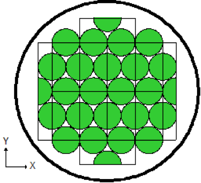
Fig. 8.1.66 Partially completed triangular pitched ARRAY in a cylinder.

UNIT 9
ARRAY 2 -10.0 -6.92822 -50.0
CYLINDER 0 1 12.4  2P50.0
HOLE 10 0.0 10.39233 0.0
HOLE 11 0.0 -10.39233 0.0
CYLINDER 2 1 12.65 2P50.0

To complete the array, the remaining half cylinders must be entered as HOLEs, as shown below. The first HOLE 1 completes the half rod at the lower left of Fig. 8.1.66. The second HOLE 1 completes the half rod at the lower center, and the third HOLE 1 completes the half rod at the lower right of Fig. 8.1.66. Similarly, the first HOLE 2 completes the half rod at the upper left of Fig. 8.1.66. The second HOLE 2 completes the half rod at the upper center, and the third HOLE 2 completes the half rod at the upper right. HOLE 3 completes the half rod at the left of Fig. 8.1.66, and HOLE 4 completes the half rod at the right. The final geometry configuration is shown in Fig. 8.1.67. UNIT 9 must be specified as the GLOBAL UNIT because it defines the overall configuration.

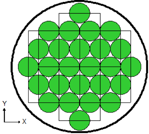
Fig. 8.1.67 Final configuration of triangular pitched ARRAY in a cylinder.

GLOBAL  UNIT 9
ARRAY 2 -10.0 -6.92822 -50.0
CYLINDER 0 1 12.4  2P50.0
HOLE 10  0.0 10.39233 0.0
HOLE 11  0.0 -10.39233 0.0
HOLE 1  -6.0  -6.92822 0.0
HOLE 1   0.0 -10.39233 0.0
HOLE 1   6.0  -6.92822 0.0
HOLE 2  -6.0   6.92822 0.0
HOLE 2   0.0  10.39233 0.0
HOLE 2   6.0   6.92822 0.0
HOLE 3 -10.0   0.0     0.0
HOLE 4  10.0   0.0     0.0
CYLINDER 2 1 12.65 2P50.0

The geometry data for Example 2b are given below.

READ GEOM

UNIT 1
ZHEMICYL-Y 1 1 2.0 50.0 -50.0

UNIT 2
ZHEMICYL+Y 1 1 2.0 50.0 -50.0

UNIT 3
ZHEMICYL-X 1 1 2.0 50.0 -50.0

UNIT 4
ZHEMICYL+X 1 1 2.0 50.0 -50.0

UNIT 5
ZHEMICYL+X 1 1 2.0 50.0 -50.0 ORIGIN -2.0 0.0
CUBOID     0 1 2P2.0 2P3.46411 2P50.0
HOLE 1  0.0  3.46411 0.0
HOLE 2  0.0 -3.46411 0.0
HOLE 3  2.0  0.0     0.0

UNIT 6
ARRAY 1 -8.0 -6.92822 -50.0

UNIT 7
ZHEMICYL+X 1 1 2.0 50.0 -50.0
CUBOID     0 1 2.0 0.0 2P6.92822 2P50.0
HOLE 3 2.0 -3.46411 0.0
HOLE 3 2.0  3.46411 0.0

UNIT 8
ZHEMICYL-X 1 1 2.0 50.0 -50.0
CUBOID     0 1 0.0 -2.0 2P6.92822 2P50.0
HOLE 3 0.0 -3.46411 0.0
HOLE 3 0.0  3.46411 0.0

UNIT 10
YZHEMICYL-Y 1 1 2.0 2P50.0
CUBOID  0 1 2P4.0 0.0 -3.46411 2P50.0
HOLE 2 -2.0 -3.46411 0.0
HOLE 2  2.0 -3.46411 0.0

UNIT 11
YZHEMICYL+Y 1 1 2.0 2P50.0
CUBOID  0 1 2P4.0 3.46411 0.0 2P50.0
HOLE 1 -2.0 3.46411 0.0
HOLE 1  2.0 3.46411 0.0

GLOBAL
UNIT 9
ARRAY 2 -10.0 -6.92822 -50.0
CYLINDER 0 1 12.4  2P50.0
HOLE 10  0.0  10.39233        0.0
HOLE 11  0.0  -10.39233       0.0
HOLE 1  -6.0    -6.92822      0.0
HOLE 1   0.0  -10.39233       0.0
HOLE 1   6.0    -6.92822      0.0
HOLE 2  -6.0     6.92822      0.0
HOLE 2   0.0   10.39233       0.0
HOLE 2   6.0     6.92822      0.0
HOLE 3 -10.0     0.0          0.0
HOLE 4  10.0     0.0          0.0
CYLINDER 2 1 12.65 2P50.0
END GEOM

READ ARRAY
ARA=1 NUX=4 NUY=2 NUZ=1  FILL F5 END FILL
ARA=2 NUX=3 NUY=1 NUZ=1 FILL 7 6 8 END FILL
END ARRAY

8.1.4.6.7. Dodecahedral pitched arrays

EXAMPLE 22.

Dodecahedral pitched ARRAYs can be described in KENO-VI by defining the UNITs that make up the ARRAY as dodecahedra and in the ARRAY data block setting TYP=DODECAHEDRAL. Since the ARRAYs are constructed by stacking dodecahedra, care must be taken to ensure the ARRAY boundary is completely enclosed within the stacked unit. Below is an example of a dodecahedral ARRAY that represents a close packed ARRAY of spheres.

The first and second UNITs are the dodecahedra that make up the ARRAY. UNIT 1 is the fuel sphere stacked in a dodecahedral lattice. UNIT 2 is a dummy UNIT used to fill in the ARRAY so the ARRAY boundary is contained within the stacked UNITs. Since the ARRAY is not moderated, UNIT 2 contains void. Fig. 8.1.68 shows an isometric, cross section view of UNITs 1 and 2.

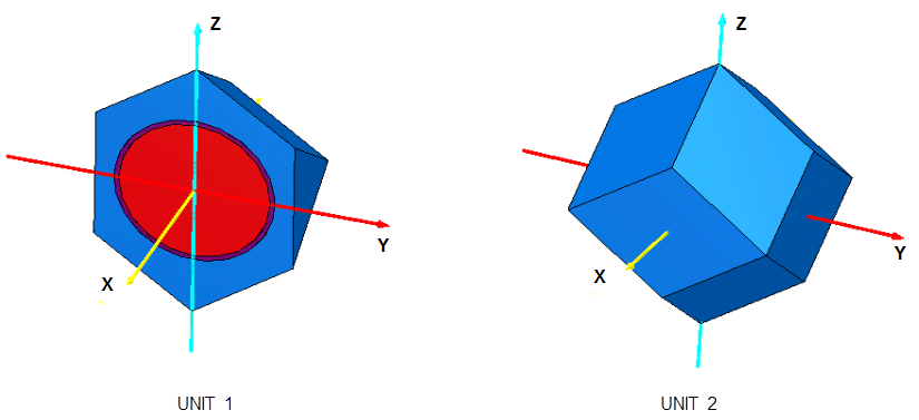
Fig. 8.1.68 Fuel cell and empty cell set up as dodecahedra.

UNIT  1
COM='SINGLE CELL FUEL CAN IN DODECAHDRON'
SPHERE       10   8.0
SPHERE       20   8.5
DODECAHEDRON 30  10.5
MEDIA  1  1  10
MEDIA  2  1  20  -10
MEDIA  0  1  30  -20
BOUNDARY     30
UNIT  2
COM='EMPTY CELL'
DODECAHEDRON 10  10.5
MEDIA  0  1  10
BOUNDARY     10

UNIT 3 is the GLOBAL UNIT that contains the ARRAY and ARRAY BOUNDARY. The ARRAY is an unmoderated triangular pitched assembly of 17 fuel spheres. Dodecahedral ARRAYs are specified by using TYP= followed by keyword dodecahedral in the array data block. The X and Y coordinates are stacked together as a square pitched ARRAY with the pitch equal to twice the dodecahedron radius. In the Z dimension, the odd Z planes (Z = 1, 3, 5, etc.) have the X and Y UNITs begin at the most negative edge of the ARRAY, while the even Z planes (Z = 2, 4, 6, etc.) have the X and Y UNITs begin one dodecahedron inscribed sphere radius in the positive direction from the most negative edge of the ARRAY. Also, the Z distance between the centers of the UNITs in successive Z planes is the square root of 2.0 times the dodecahedron radius (or the dodecahedron diameter divided by the square root of 2.0). Fig. 8.1.69 and Fig. 8.1.70 show X-Y cross sectional color plots of the assembly at an odd and even Z plane.

GLOBAL UNIT 3
COM='17 CLOSE PACKED FUEL SPHERES IN A CYLINDER'
CYLINDER  10  41.0  44.5   0.0
CYLINDER  20  42.0  44.5  -1.0
ARRAY  1  10 PLACE 3 3 1 3*0.0
MEDIA  3  20  -10
BOUNDARY 20

READ ARRAY GBL=1 ARA=1 TYP=DODECAHEDRAL NUX=5 NUY=5 NUZ=5
FILL 25*2
     6*2  2*1  3*2  2*1  12*2
     6*2  3*1  2*2  3*1  2*2  3*1  6*2
     6*2  2*1  3*2  2*1  12*2
     25*2 END FILL  END ARRAY

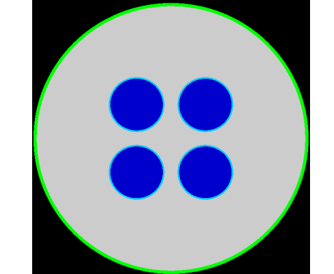
Fig. 8.1.69 X-Y slice of dodecahedral array at even level Z = 2.

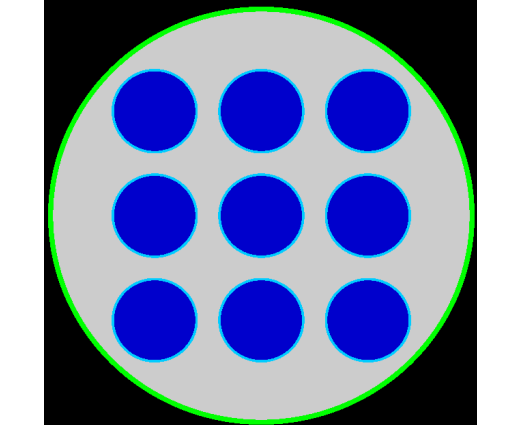
Fig. 8.1.70 X-Y slice of dodecahedral array at odd level Z = 3.

The overall problem description is shown below. The cross section library would be generated in a separate CSAS-MG step.

Data description of Example 22.

=KENOVI
CLOSE PACKED DODECAHEDRAL ARRAY 17 FUEL SPHERES IN A CYLINDER
READ PARAMETERS LNG=20000 LIB=4 END PARAMETERS
READ MIXT SCT=2
MIX=1 NCM=8 92235 1.37751E-03  92238 9.92354E-05  8016 3.32049E-02
       9019 2.95349E-03  1001 6.05028E-02
MIX=2 NCM=14 13027 6.02374E-02
MIX=3 NCM=14 13027 6.02374E-02
END MIXT
READ GEOMETRY
UNIT  1
COM='SINGLE CELL FUEL CAN IN DODECAHDRON'
SPHERE       10   8.0
SPHERE       20   8.5
DODECAHEDRON 30  10.5
MEDIA  1  1  10
MEDIA  2  1  20  -10
MEDIA  0  1  30  -20
BOUNDARY     30
UNIT  2
COM='EMPTY CELL'
DODECAHEDRON 10  10.5
MEDIA  0  1  10
BOUNDARY     10
GLOBAL UNIT 3
COM='9 CLOSE PACKED FUEL SPHERES IN A CYLINDER'
CYLINDER  10  41.0  44.5   0.0
CYLINDER  20  42.0  44.5  -1.0
ARRAY  1  10 PLACE 3 3 1 3*0.0
MEDIA  3  1 20  -10
BOUNDARY 20
END GEOMETRY
READ ARRAY GBL=1 ARA=1 TYP=DODECAHEDRAL NUX=5 NUY=5 NUZ=5
FILL 25*2
     6*2  2*1  3*2  2*1  12*2
     6*2  3*1  2*2  3*1  2*2  3*1  6*2
     6*2  2*1  3*2  2*1  12*2
     25*2 END FILL  END ARRAY
READ PLOT
TTL='DODECAHEDRAL ARRAY, 4 SPHERES - Z LEVEL = 2'
XUL=-43.0  YUL=43.0  ZUL=14.85  XLR=43.0  YLR=-43.0  ZLR=14.85
UAX=1  VDN=-1  NAX=640    END  PLT0
TTL='DODECAHEDRAL ARRAY, 9 SPHERES - Z LEVEL = 3'
XUL=-43.0  YUL=43.0  ZUL=29.70  XLR=43.0  YLR=-43.0  ZLR=29.70
UAX=1  VDN=-1  NAX=640    END  PLT1
END PLOT
END DATA
END

8.1.4.7. Alternative sample problem mockups

The geometry data for KENO can often be described correctly in several ways. Some alternative geometry descriptions are given here for sample problems C.12 and C.13. (See Sect. 8.1.8.3 of the KENO manual.)

8.1.4.7.1. Sample Problem C.12, First Alternative

This mockup maintains the same overall unit dimensions that were used in sample problem C.12. In sample problem C.12, the origin of UNIT 1, the solution cylinder, is at the center of the unit; the origin of UNITs 2, 3, 4, and 5, the metal cylinders, are at the center of the cylinders. In this mockup, the unit numbers remain the same and the origin of each unit is at the center of the unit. In each unit the cylinder is offset by specifying the position of its centerline relative to the origin of the UNIT.

KENO V.a:

READ GEOM
UNIT 1
CYLINDER  2 1 9.525 8.89 -8.89
CYLINDER  3 1 10.16 9.525 -9.525
CUBOID    0 1 10.875 -10.875 10.875 -10.875 10.24 -10.24
UNIT 2
CYLINDER  1 1 5.748 9.3975 -1.3975 ORIG 4.285 4.285
CUBOID    0 1 10.875 -10.875 10.875 -10.875 10.24 -10.24
UNIT 3
CYLINDER  1 1 5.748 9.3975 -1.3675 ORIG 4.285 -4.285
CUBOID    0 1 10.875 -10.875 10.875 -10.875 10.24 -10.24
UNIT 4
CYLINDER  1 1 5.748 1.3675 -9.3975 ORIG 4.285 4.285
CUBOID    0 1 10.875 -10.875 10.875 -10.875 10.24 -10.24
UNIT 5
CYLINDER  1 1 5.748 1.3675 -9.3975 ORIG 4.285 -4.285
CUBOID    0 1 10.875 -10.875 10.875 -10.875 10.24 -10.24
END GEOM
READ ARRAY  NUX=2 NUY=2 NUZ=2 FILL 2 1 3 1 4 1 5 1 END ARRAY

KENO-VI:

READ GEOM
UNIT 1
CYLINDER 1  9.525 8.89 -8.89
CYLINDER 2  10.16 9.525 -9.525
CUBOID  3   10.875 -10.875 10.875 -10.875 10.24 -10.24
MEDIA 2 1 1
MEDIA 3 1 2 -1
MEDIA 0 1 3 -2
BOUNDARY  3
UNIT 2
CYLINDER 1  5.748 9.3975 -1.3675 ORIG  X=4.285 Y=4.285
CUBOID  2   10.875 -10.875 10.875 -10.875 10.24 -10.24
MEDIA 1 1 1
MEDIA 0 1 2 -1
BOUNDARY  2
UNIT 3
CYLINDER 1  5.748 9.3975 -1.3675 ORIG X=4.285 Y=-4.285
CUBOID  2   10.875 -10.875 10.875 -10.875 10.24 -10.24
MEDIA 1 1 1
MEDIA 0 1 2 -1
BOUNDARY  2
UNIT 4
CYLINDER 1  5.748 1.3675 -9.3975 ORIG X=4.285 Y=4.285
CUBOID  2   10.875 -10.875 10.875 -10.875 10.24 -10.24
MEDIA 1 1 1
MEDIA 0 1 2 -1
BOUNDARY  2
UNIT 5
CYLINDER 1  5.748 1.3675 -9.3975 ORIG X=4.285 Y=-4.285
CUBOID  2   10.875 -10.875 10.875 -10.875 10.24 -10.24
MEDIA 1 1 1
MEDIA 0 1 2 -1
BOUNDARY  2
GLOBAL UNIT 6
CUBOID 1 21.75 -21.75 21.75 -21.75 20.48 -20.48
ARRAY 1 PLACE 1 1 1 -10.875 -10.875 -10.24
BOUNDARY  1
END GEOM
READ ARRAY ARA=1  NUX=2 NUY=2 NUZ=2 FILL 2 1 3 1 4 1 5 1 END ARRAY

8.1.4.7.2. Sample Problem C.12, Second Alternative

In this mockup, the outer boundaries of the system are made as close fitting as possible on all six faces. The origin of each UNIT is located at the center of the cylinder. UNITs 1, 3, 5, and 7 contain the metal cylinders. UNITs 2, 4, 6, and 8 contain the solution cylinders.

KENO V.a:

READ GEOM
UNIT 1
CYLINDER 1 1 5.748 5.3825 -5.3825
CUBOID   0 1 6.59 -5.748 6.59 -14.445 6.225 -13.54
UNIT 2
CYLINDER  2 1 9.525 8.89 -8.89
CYLINDER  3 1 10.16 9.525 -9.525
CUBOID    0 1 10.16 -10.875 10.875 -10.16 10.24 -9.525
UNIT 3
CYLINDER  1 1 5.748 5.3825 -5.3825
CUBOID    0 1 6.59 -5.748 14.444 -6.59 6.225 -13.54
UNIT 4
CYLINDER   2 1 9.525 8.89 -8.89
CYLINDER   3 1 10.16 9.525 -9.525
CUBOID     0 1 10.16 -10.875 10.16 -10.875 10.24 -9.525
UNIT 5
CYLINDER  1 1 5.748 5.3825 -5.3825
CUBOID    0 1 6.59 -5.748 6.59 -14.445 13.54 -6.225
UNIT 6
CYLINDER   2 1 9.525 8.89 -8.89
CYLINDER   3 1 10.16 9.525 -9.525
CUBOID     0 1 10.16 -10.875 10.875 -10.16 9.525 -10.24
UNIT 7
CYLINDER  1 1 5.748 5.3825 -5.3825
CUBOID    0 1 6.59 -5.748 14.445 -6.59 13.54 -6.225
UNIT 8
CYLINDER   2 1 9.525 8.89 -8.89
CYLINDER   3 1 10.16 9.525 -9.525
CUBOID     0 1 10.16 -10.875 10.16 -10.875 9.525 -10.24
READ ARRAY  NUX=2 NUY=2 NUZ=2 FILL 6I1 8 END FILL END ARRAY

KENO-VI:

READ GEOM
UNIT 1
CYLINDER 1 5.748 5.3825 -5.3825
CUBOID  2  6.59 -5.748 6.59 -14.445 6.225 -13.54
MEDIA 1 1 1
MEDIA 0 1 2 -1
BOUNDARY  2
UNIT 2
CYLINDER 1  9.525 8.89 -8.89
CYLINDER 2  10.16 9.525 -9.525
CUBOID  3   10.16 -10.875 10.875 -10.16 10.24 -9.525
MEDIA 2 1 1
MEDIA 3 1 2 -1
MEDIA 0 1 3 -2
BOUNDARY  3
UNIT 3
CYLINDER  1 5.748 5.3825 -5.3825
CUBOID  2   6.59 -5.748 14.444 -6.59 6.225 -13.54
MEDIA 1 1 1
MEDIA 0 1 2 -1
BOUNDARY  2
UNIT 4
CYLINDER 1  9.525 8.89 -8.89
CYLINDER 2  10.16 9.525 -9.525
CUBOID   3   10.16 -10.875 10.16 -10.875 10.24 -9.525
MEDIA 2 1 1
MEDIA 3 1 2 -1
MEDIA 0 1 3 -2
BOUNDARY  3
UNIT 5
CYLINDER 1 5.748 5.3825 -5.3825
CUBOID   2  6.59 -5.748 6.59 -14.445 13.54 -6.225
MEDIA 1 1 1
MEDIA 0 1 2 -1
BOUNDARY  2
UNIT 6
CYLINDER 1  9.525 8.89 -8.89
CYLINDER 2  10.16 9.525 -9.525
CUBOID   3   10.16 -10.875 10.875 -10.16 9.525 -10.24
MEDIA 2 1 1
MEDIA 3 1 2 -1
MEDIA 0 1 3 -2
BOUNDARY  3
UNIT 7
CYLINDER 1  5.748 5.3825 -5.3825
CUBOID  2   6.59 -5.748 14.445 -6.59 13.54 -6.225
MEDIA 1 1 1MEDIA 0 1 2 -1
BOUNDARY  2
UNIT 8
CYLINDER 1  9.525 8.89 -8.89
CYLINDER 2  10.16 9.525 -9.525
CUBOID  3    10.16 -10.875 10.16 -10.875 9.525 -10.24
MEDIA 2 1 1
MEDIA 3 1 2 -1
MEDIA 0 1 3 -2
BOUNDARY  3
GLOBAL UNIT 9
CUBOID 1 20.035 -12.748 20.67 -20.67 19.765 -19.765
ARRAY 1 1 PLACE 1 1 1 -7.00 -6.225 -6.225
BOUNDARY  1
END GEOM
READ ARRAY ARA=1  NUX=2 NUY=2 NUZ=2 FILL 6I1 8 END FILL END ARRAY

8.1.4.7.3. Sample Problem C.13, Alternative

This mockup maintains the same overall UNIT dimensions that were used in sample problem C.13, (KENO Manual, Sect. 8.1.8.3). In sample problem C.13, the origin of UNITs 1, 2, and 3 is located at the center of the base of the uranium metal cuboid. In this mockup, the origin of UNITs 1 and 2 is located at the center of the cylinder. In UNIT 3, the origin is at the center of the UNIT.

KENO V.a:

READ GEOM
UNIT 1
CUBOID  1 1 0.2566 -12.4434 6.35 -6.35 3.81 -3.81
CYLINDER  0 1 13.97 3.81 -3.81
CYLINDER  1 1 19.05 3.81 -3.81
CUBOID  0 1 19.05 -19.05 19.05 -19.05 3.81 -3.81
UNIT 2
CUBOID  1 1 12.4434 -0.2566 6.35 -6.35 4.28 -4.28
CYLINDER  0 1 13.97 4.28 -4.28
CYLINDER  1 1 19.05 4.28 -4.28
CUBOID  0 1 19.05 -19.05 19.05 -19.05 4.28 -4.28
UNIT 3
CUBOID  1 1 12.4434 -0.2566 6.35 -6.35 1.308 -1.308
CUBOID  0 1 19.05 -19.05 19.05 -19.05 1.308 -1.308
END GEOM
READ ARRAY  NUX=1 NUY=1 NUZ=3  FILL 1 2 3 END ARRAY

KENO-VI:

READ GEOM
UNIT 1
CUBOID  1 0.2566 -12.4434 6.35 -6.35 3.81 -3.81
CYLINDER 2  13.97 3.81 -3.81
CYLINDER 3  19.05 3.81 -3.81
CUBOID 4  19.05 -19.05 19.05 -19.05 3.81 -3.81
MEDIA 1 1 1
MEDIA 0 1 2 -1
MEDIA 1 1 3 -2 -1
MEDIA 0 1 4 -3 -2 -1
BOUNDARY  4
UNIT 2
CUBOID  1 12.4434 -0.2566 6.35 -6.35 4.28 -4.28
CYLINDER 2 13.97 4.28 -4.28
CYLINDER 3 19.05 4.28 -4.28
CUBOID 4  19.05 -19.05 19.05 -19.05 4.28 -4.28
MEDIA 1 1 1
MEDIA 0 1 2 -1
MEDIA 1 1 3 -2 -1
MEDIA 0 1 4 -3 -2 -1
BOUNDARY  4
UNIT 3
CUBOID 1 12.4434 -0.2566 6.35 -6.35 1.308 -1.308
CUBOID 2 19.05 -19.05 19.05 -19.05 1.308 -1.308
MEDIA 1 1 1
MEDIA 0 1 2 -1
BOUNDARY  2
GLOBAL UNIT 4
CUBOID 1 19.05 -19.05 19.05 -19.05 6.896  -11.90
ARRAY 1 1 PLACE 1 2 1 0.0 0.0 0.0
BOUNDARY  1
END GEOM
READ ARRAY ARA=1  NUX=1 NUY=1 NUZ=3  FILL 1 2 3 END ARRAY

8.1.4.8. Initial starting distributions with Start data

Sect. 8.1.3.8 discusses the input directions for entering different starting distributions in the start data input block. The following start type 0 and start type 6 examples demonstrate how KENO codes process the entered start data parameters.

Example-1:

An 8 cm radius fissile sphere without a start data block is modeled with both KENO-VI and KENO V.a geometries. Start type 0, which is the default starting option, is used, and neutrons are started uniformly in the entire volume defined by the outermost geometry (fissile sphere).

KENO-VI:

...
 read geometry
    global unit 1
       sphere 1  8
       media 1 1 1
       boundary 1
 end geometry
end data
end

KENO V.a:

' input without global unit
...
 read geometry
    unit 1
       sphere 1 1 8
 end geometry
end data
end


' input with global unit
...
 read geometry
    global unit 1
       sphere 1 1 8
 end geometry
end data
end

Example-2:

This input models a simple 2 \(\times\) 2 \(\times\) 2 array of fissile cylinders with the default starting option, which is start type 0. In this array problem, XSM, YSM, and ZSM are defaulted to the minimum X, Y, and Z coordinates of the global array, and XSP, YSP, and ZSP are defaulted to the maximum coordinates of the global array. A bounding box is constructed with these values, and neutrons are started at the points uniformly sampled inside the fissile cylinders within this cuboid (For KENO V.a model, the cuboid is defined by +x=27.48, -x=0.0, +y=27.48, -y=0.0, +z= 26.02, -z= 0.0, and for KENO-VI model, it is defined by +x=13.74, -x=-13.74, +y=13.74, -y=-13.74, +z= 13.01, -z=-13.01).

KENO-VI:

...
 read geometry
    unit 1
       cylinder 1 5.748 2p5.3825
       cuboid   2 4p6.87 2p6.505
       media 1 1 1
       media 0 1 2 -1
       boundary 2
    global unit 2
       cuboid  10 4p13.74 2p13.01
       array 1 +10 place 1 1 1 2r-6.87 -6.505
       boundary 10
 end geometry
 read array
   gbl=1 ara=1 nux=2 nuy=2 nuz=2 fill f1  end fill
 end array
end data
end

KENO V.a:

' input with a global array
...
 read geometry
     unit 1
        cylinder 1 1 5.748 5.3825 -5.3825
        cuboid  0 1 6.87 -6.87 6.87 -6.87 6.505 -6.505
 end geometry
 read array
    gbl=1 ara=1 nux=2 nuy=2 nuz=2 fill f1  end fill
 end array
end data
end

Example-3:

Neutrons are started uniformly throughout the fissile materials in a user-defined box that is inside the outermost geometry (+x=3.0 -x=-3.0 +y= 1.0 -y=-1.0 +z= 2.0 -z=-2.0).

KENO-VI:

...
 read geometry
    global unit 1
       sphere 1  8
       media 1 1 1
       boundary 1
 end geometry

 READ START
    NST=0
    XSP=3.0 XSM=-3.0 YSP=1.0 YSM=-1.0 ZSP=2.0 ZSM=-2.0
 END START

end data
end

Example-4:

This test case is another example of the start type 0 specification with a user-defined cuboid, but whole cuboid is not inside the outermost geometry. KENO V.a immediately terminates the execution with some error messages since some starting points are sampled outside the outermost geometry.

Unlike KENO V.a, KENO-VI continues the sampling process by discarding these points, which are outside the global geometry, until all starting points have been successfully sampled throughout the fissile regions inside the global unit.

KENO-VI:
...
 read geometry
    global unit 1
       sphere 1  8
       media 1 1 1
       boundary 1
 end geometry

 READ START
    NST=0
    XSP=10.0 XSM=-10.0 YSP=10.0 YSM=-10.0 ZSP=10.0 ZSM=-10.0
 END START

end data
end

Note

Note that the KENO-VI sampling process for such a case will be terminated if

• the first starting point has not been sampled in tbtch minutes. tbtch is the time per generation in minutes, defaulted to 10 minutes. User can control this with parameter TBA= in parameter input; see Sect. 8.1.3.3 for details, or

• all points have not been successfully sampled inside the global units in total tbtch \(\times\) 9.5 minutes.

Example-5:

This test input demonstrates how KENO-VI performs source sampling with the default starting type (start type 0) if the boundary definition vector of the global unit has the multiple body labels. For such cases, KENO-VI starts neutrons at the points that are uniformly sampled in the first body entered in the boundary definition vector of the global unit if and only if none of translation and transformation operations are performed on this body. For this KENO-VI specific example, all starting points are sampled throughout the fissile materials inside the cylinder 3.

KENO-VI:

...
 read geometry
    global unit 1
       sphere 1 8.741
       sphere 2 10.0
       cylinder 3 8.0 2p8.0
       media 1 1 1
       media 2 1 2 3 -1
       BOUNDARY  3 2
 end geometry

end data
end

Example-6:

Start type 0 specification with one or more missing optional parameters; their default values (0.0) are used to construct a cuboid, and neutrons are started uniformly throughout the fissile materials in this box (+x=3.0 -x=0.0 +y= 1.0 -y=0.0 +z=0.0 -z=-2.0).

KENO-VI:

...
 read geometry
    global unit 1
       sphere 1  8
       media 1 1 1
       boundary 1
 end geometry

 READ START
    NST=0
    XSP=3.0 YSP=1.0 ZSM=-2.0
 END START

end data
end

Note

In start data input, user-defined cuboid shape is considered as a deformed cuboid shape if the minimum and maximum bounds in any dimension are equal entries (XSP = XSM or/and YSP = YSM or/and ZSP = ZSM). Deformed shape specification is a legitimate input specification across SCALE sequences (i.e., a box is deformed into a plane if minimum and maximum bounds in one dimension are the same, e.g., +x = -x). In such a case, user-defined entries for XSM, XSP, YSM, YSP, ZSM, and ZSP are ignored, and source sampling is performed throughout the volume defined by the outermost geometry card.

The following two examples with start type 0 demonstrate code behavior for the deformed shapes for start types 0, 1, 2, and 7.

Example-7:

Box defined with missing ZSM, and ZSP is considered as a deformed cuboid since these parameters are identical after defaulting their values to 0.0. Instead of this deformed cuboid box, neutrons are started uniformly throughout the fissile materials in the global unit.

KENO-VI:

...
 read geometry
    global unit 1
       sphere 1  8
       media 1 1 1
       boundary 1
 end geometry

 READ START
    NST=0
    XSP=3.0 XSM=-3.0 YSP=1.0 YSM=-1.0
 END START

end data
end

Example-8:

A box defined with identical XSM and XSP entries is considered as a deformed cuboid since these parameters are identical after defaulting their values to 0.0. Instead of this deformed cuboid box, neutrons are started uniformly throughout the fissile materials in the global unit.

KENO-VI:

...
 read geometry
    global unit 1
       sphere 1  8
       media 1 1 1
       boundary 1
 end geometry

 READ START
    NST=0
    XSP=3.0 XSM=3.0 YSP=1.1 YSM=-2.1 ZSP=4.0 ZSM=-4.1
 END START

end data
end

In the start type 6 capability, the selection process for the initial fission source points depends on the values of the last LNU value and number per generation (parameter NPG= in the parameter input Sect. 8.1.3.3). The following rules are applied when selecting the starting points:

• Start NPG initial fission neutrons at first-NPG starting points defined by start type 6 data if NPG < LNU. Remaining starting points beyond NPG will be discarded.

• Start NPG initial fission neutrons at LNU starting points defined by start type 6 data if NPG = LNU.

• Start LNU initial fission neutrons at the starting points defined by start type 6 data, then randomly select the remaining fission source points (NPG-LNU) from these starting points if NPG > LNU.

Warning

It is the user’s responsibility to enter all arbitrary starting points consistent with the geometry specified. Both KENO V.a and KENO-VI terminate the execution with several error messages if any user-specified starting point entered is outside the outermost geometry.

Example-9:

In this example, 120 starting points have been defined by start type 6 data, and NPG=100 starting points are selected from the defined start type 6 data, 25 neutrons are started at the point (2.0, 3.0, 0.0), 20 neutrons are started at the point (3.0, -2.0, -6.0), and the remaining 55 neutrons are started at (3.0, 5.2, 1.0). All selected points are relative to the global coordinate system. Missing TFX entry in the last start type 6 data set is set to the last updated TFX value which is 3.0.

KENO-VI:

...

 READ PARAMETER
    NPG=100
 END PARAMETER

 read geometry
    global unit 1
       sphere 1  8
       media 1 1 1
       boundary 1
 end geometry

 READ START
    NST=6
    TFX=2.0 TFY= 3.0 TFZ=0.0  LNU=25
    TFX=3.0 TFY=-2.0 TFZ=-6.0 LNU=45
            TFY=5.2  TFZ=1.0  LNU=120
 END START

end data
end

Example-10:

In this example, only 45 starting points have been defined by start type 6 data. The first 25 neutrons are started at the point (2.0, 0.0, 0.0), and 20 neutrons are started at the point (2.0, 3.0, -6.0). The remaining 55 neutrons are started at the points randomly selected from these starting points. All selected points are relative to the global coordinate system. Missing TFY and TFZ entries are defaulted to 0.0 in the first start type 6 data set. The missing TFX entry in the last start type 6 data set is set to the last updated TFX value, which is 2.0 (from the previous start type 6 data set).

KENO-VI:

...

 READ PARAMETER
    NPG=100
 END PARAMETER

 read geometry
    global unit 1
       sphere 1  8
       media 1 1 1
       boundary 1
 end geometry

 READ START
    NST=6
    TFX=2.0          LNU=25
    TFY=3.0 TFZ=-6.0 LNU=45
 END START

end data
end

Example-11:

In this example, 35 neutrons are started at the point (0.0, 0.0, 0.0) relative to the global array element (2,1,1), and the remaining 65 neutrons are started at the point (2.0, 1.0, 3.0) relative to the global array element (1,2,2). The missing TFX, TFY, and TFZ entries in each data set are defaulted to 0.0.

KENO V.a:

...

 READ PARAMETER
    NPG=100
 END PARAMETER

 read geometry
    unit 1
       cylinder 1 1 5.748 5.3825 -5.3825
       cuboid  0 1 6.87 -6.87 6.87 -6.87 6.505 -6.505
 end geometry

 read array
    gbl=1 ara=1 nux=2 nuy=2 nuz=2 fill f1  end fill
 end array

 READ START
    NST=6
    NXS=2 NYS=1 NZS=1 LNU=35
        TFX=2.0 TFY=1.0 TFZ=3.0 NXS=1 NYS=2 NZS=2 LNU=100
 END START

end data
end

Start type 6 is capable of reading starting points from an ASCII start data file, which could be created by writing starting points from a previous calculation, defined by RDU in a start type 6 data set. See Sect. 8.1.3.8.1 for the details about a typical ASCII start data file currently supported.

Reading starting data from multiple ASCII start data files is also supported. Similarly, single or multiple start type 6 date sets with RDU specification can be used together with other start type 6 data sets discussed above. The following examples demonstrate this capability.

Example-12:

In this example, all starting points stored in the ASCII start data file sample.src are read, and NPG neutrons are started at these points. If the number of starting points (last LNU read from the file) is less than NPG, LNU number of neutrons are started at the points read, and the remaining neutrons (NPG-LNU) are started at the points randomly sampled from the starting points already read. The starting points beyond NPG are discarded if NPG is less than the number of starting points read.

...
READ START
   NST=6
   RDU=sample.src
END START

Example-13:

The first 32 starting points stored in the ASCII start data file sample.src are read, and NPG neutrons are started at these points. If NPG > LNU = 32, then 32 neutrons are started at these starting points, and the remaining neutrons are started at the points randomly sampled from these 32 starting points. The starting points beyond NPG is discarded if NPG < 32.

...
READ START
   NST=6
   RDU=sample.src LNU=32
END START

Note

Reading starting data from multiple ASCII start data files is also supported. Similarly, single or multiple start type 6 date sets with the RDU specification can be used together with other start type 6 data sets discussed above. The following examples demonstrates this capability.

Example-14:

A total of 30 starting points are read both from the specified ASCII start data files and from the start type 6 data set defined with TFX, TFY, and TFZ. Neutrons are started at these points. If there is a shortage of starting points (NPG >> last LNU), then the required number of starting points is randomly sampled from these 30 starting points.

...
READ START
   NST=6
   RDU=sample1.src LNU=10
   RDU=sample2.src LNU=25
       TFX=1.0 TFY=3.0 TFZ=4.0 LNU=30
END START

8.1.4.9. Biasing or weighting data for multigroup mode

Sect. 8.1.4.6.3 discusses the basis of weighting or biasing. The use of biasing data in reflected problems has been illustrated in Examples 9, 10, and 11 of Sect. 8.1.4.6. Sect. 8.1.3.7 discusses the input directions for entering biasing data.

Every shape card in KENO V.a, or MEDIA card in KENO-VI requires a bias ID to associate that geometry region with a biasing or weighting function. A biasing or weighting function is a set of energy-dependent values of the average weight that are applicable in a given region. The default function for all bias IDs is constant through all energy groups and is defined to be the default value of weight average which can be specified in the parameter data. A bias ID can be associated with a biasing function (other than default) by specifying it in the biasing input data. This function can be chosen from the weighting library, or it can be entered from records. Table 8.1.25 lists the materials and energy group structures for biasing functions available from the weighting library.

Caution

In general, the use of biasing should be restricted to external reflectors unless the user has generated correct biasing functions for other applications. Improper use of biasing functions can result in erroneous answers without giving any indication that they are invalid. Caution should be exercised in the generation and use of biasing functions.

Biasing functions are most applicable to thick external reflectors. Their use can significantly reduce the amount of computer time required to obtain answers in KENO. If the user wishes to use a biasing function for a concrete reflector, for example, the following steps must be included in preparing the input data:

1. The geometry region data must define the shape and dimensions of the reflector using the mixture ID for concrete and a sequence of bias IDs that associate the geometry region with the appropriate interval of the concrete weighting function. CAUTION: THE THICKNESS AND SEQUENTIAL LOCATION OF EACH REGION USING BIASING FUNCTIONS MUST MATCH OR VERY NEARLY MATCH THE INCREMENT THICKNESS AND ORDER OF THE WEIGHTING DATA. NO CHECK IS MADE ON THE REQUIREMENT. IT IS THE USER’S RESPONSIBILITY TO ENSURE CONSISTENCY.

2. Biasing data must be entered. This must include the material ID for the reflector material (from Table 8.1.25 or as specified on records) and a beginning and ending bias ID. The beginning bias ID is used to select the first set of energy-dependent average weights, and the subsequent sets of energy-dependent average weights are assigned consecutive IDs until the ending bias ID is reached.

Small deviations in reflector region thickness are allowed, such as using three generated regions with a thickness per region of 5.08 cm to generate a 15.24 cm thick reflector of concrete, or using five generated regions with a thickness per region of 3.048 cm to generate a 15.24 cm thick reflector of water. See Table 8.1.25 for a list of the increment thicknesses for the materials in the weighting library. It is acceptable for the thickness of the last reflector region to be significantly different than the increment thickness. For example, a reflector record specifying five generated regions with a thickness per region of 3.0 cm could be followed by a reflector record specifying one region with a thickness per region of 0.24 cm. Assuming that material 2 is water and a 15.24 cm thick cuboidal reflector of water is desired, the required reflector description and biasing data could be entered as follows:

KENO V.a:

REFLECTOR 2 2 6*3.0  5
REFLECTOR 2 7 6*0.24 1
READ BIAS ID=500 2 7 END BIAS

KENO-VI:

GLOBAL UNIT 1
CUBOID 1 6P10.0
CUBOID 2 6P13.0
CUBOID 3 6P16.0
CUBOID 4 6P19.0
CUBOID 5 6P22.0
CUBOID 6 6P25.0
CUBOID 7 6P25.24
MEDIA 1 1 1
MEDIA 2 2 2 -1
MEDIA 2 3 3 -2
MEDIA 2 4 4 -3
MEDIA 2 5 5 -4
MEDIA 2 6 6 -5
MEDIA 2 7 7 -6
BOUNDARY  7
READ BIAS ID=500 2 7 END BIAS

The same 15.24 cm thick reflector can be described by including the extra 0.24 cm in the last region as shown below:

KENO V.a:

REFLECTOR 2 2 6*3.0  4
REFLECTOR 2 6 6*3.24 1
READ BIAS  ID=500 2 6 END BIAS

KENO-VI:

GLOBAL UNIT 1
CUBOID 1 6P10.0
CUBOID 2 6P13.0
CUBOID 3 6P16.0
CUBOID 4 6P19.0
CUBOID 5 6P22.0
CUBOID 6 6P25.24
MEDIA 1 1 1
MEDIA 2 2 2 -1
MEDIA 2 3 3 -2
MEDIA 2 4 4 -3
MEDIA 2 5 5 -4
MEDIA 2 6 6 -5
BOUNDARY  6
READ BIAS ID=500 2 6 END BIAS

Here the weighting functions associated with bias IDs 2, 3, 4, and 5 each have a thickness of 3.0 cm, corresponding exactly to the increment thickness for water in Table 8.1.25 Bias ID 6 is used for the last generated region which is 3.24 cm thick.

The following examples illustrate the use of biasing data. Suppose the user wishes to use the weighting function for water from Table 8.1.25 for bias IDs 2 through 6. The biasing input data would then be:

READ BIAS  ID=500 2 6 END BIAS

The energy-dependent values of weight average for the first 3 cm interval of water will be used for weighting the geometry regions that specify a bias ID of 2. The energy-dependent values of weight average for the second 3 cm interval of water will be used for geometry regions that specify a bias ID of 3, etc. Thus, the energy-dependent values of weight average for the fifth 3 cm interval of water will be used for geometry regions that specify a bias ID of 6. Geometry regions that use bias IDs other than 2, 3, 4, 5, and 6 will use the default value of weight average that is constant for all energies as a biasing function.

Several sets of biasing data can be entered at once. Assume the user wishes to use the weighting function for concrete from Table 8.1.25 for bias IDs 2 through 4 and the weighting function for water for bias IDs 5 through 7. The appropriate input data block is the following:

READ BIAS  ID=301 2 4 ID=500 5 7 END BIAS

The energy-dependent values of weight average for the first 5 cm interval of concrete will be used for the geometry regions that specify a bias ID of 2, the energy-dependent values of weight average for the second 5 cm interval of concrete will be used for the geometry regions that specify a bias ID of 3, and the energy-dependent values of weight average for the third 5 cm interval of concrete will be used for the geometry regions that specify a bias ID of 4. The energy-dependent values of weight average for the first 3 cm interval of water will be used for geometry regions that specify a bias ID of 5, the values for the second 3 cm interval of water will be used for geometry regions that specify a bias ID of 6, and the values for the third 3 cm interval of water will be used for geometry regions that specify a bias ID of 7. The default value of weight average will be used for all bias IDs outside the range of 2–7.

If the biasing data block defines the same bias ID more than once, the value that is entered last supersedes previous entries. Assuming that the following data block is entered,

READ BIAS  ID=400 2 7 ID=500 5 7 END BIAS

the data for paraffin (ID=400) will be used for bias IDs 2, 3, and 4, and the data for water (ID=500) will be used for bias IDs 5, 6, and 7.

EXAMPLE 1. USE OF BIASING DATA

It is assumed that a 5 cm radius sphere of material 2 is reflected by a 20 cm thickness of material 1 (concrete). The concrete reflector is spherical and close fitting upon the sphere of material 2. The mixing table must specify material 1 and material 2. Material 1 must be defined as concrete. The geometry and biasing data should be entered as follows:

KENO V.a:

READ GEOM
SPHERE 2 1 5.0
REPLICATE 1 2 5.0 4
END GEOM
READ BIAS ID=301 2 5 END BIAS

KENO-VI:

READ GEOM
GLOBAL UNIT 1
SPHERE 1 5.0
SPHERE 2 10.0
SPHERE 3 15.0
SPHERE 4 20.0
SPHERE 5 25.0
MEDIA 2 1 1
MEDIA 1 2 2 -1
MEDIA 1 3 3 -2
MEDIA 1 4 4 -3
MEDIA 1 5 5 -4
BOUNDARY  5
END GEOM
READ BIAS ID=301 2 5 END BIAS

The bias ID for the first generated region is 2, the second is 3, the third is 4, and the fourth is 5. The biasing data block specifies that the biasing function for material ID 301 (concrete) will be used from the weighting library. The bias ID to which the energy-dependent weighting function for the first 5.0 cm interval of concrete is applied is 2; the energy-dependent weighting function for the fourth 5 cm interval of concrete is applied to the fourth generated geometry region. This generated region has a bias ID of 5.

In KENO V.a, Example 1 can also be described without using a reflector record as shown below. The records that are generated by the reflector record in the previous set of data are identical to the last four spheres in this mockup.

EXAMPLE 1. Use of biasing without a reflector record.

KENO V.a:

READ GEOM
SPHERE 2 1 5.0
SPHERE 1 2 10.0
SPHERE 1 3 15.0
SPHERE 1 4 20.0
SPHERE 1 5 25.0
END GEOM
READ BIAS  ID=301 2 5 END BIAS

8.1.4.10. Color plots

Plots are generated only if a plot data block has been entered for the problem and PLT=NO has not been entered in the parameter data or the plot data. See Sect. 8.1.3.11 for a description of plot data. When a plot is to be made, the user MUST correctly specify the upper left-hand corner of the plot with respect to the origin of the plot. The origin of a plot is defined as the origin of the GLOBAL UNIT.

Plots can represent mixture numbers, unit numbers, or bias ID numbers. A title can be entered for each plot. If plot titles are omitted, the title of the KENO case will be printed for each plot title until a plot title is entered. If a plot title is entered and a subsequent plot title is omitted, the last plot title prior to the omitted one will be used for the omitted one.

The upper left and lower right coordinates define the area (i.e., the slice and its location) for which the plot is to be made. The direction cosines across the plot and the direction cosines down the plot define the direction of the vector across the plot and the vector down the plot with respect to the geometry coordinate system. One of the simplest ways of generating a plot is to specify the desired coordinates of the upper left and lower right corners of the plot. Then one must determine which plot axis is to be across the plot and which is to be down. The sign of the direction cosine should be consistent with the direction of that component when moving from the upper left to lower right corner. For example, to draw a plot of an X-Z slice at Y = 5.0 with X across the plot and Z down the plot for a system whose X coordinates ranges from 0.0 to 10.0 and whose Z coordinates range from 0.0 to 20.0, the upper left coordinate could be XUL=0.0 YUL=5.0 ZUL=20.0 and the lower right coordinates could be XLR=10.0 YLR=5.0 ZLR=0.0. Since X is to be plotted across the plot with X = 0.0 at the left and X = 10.0 at the right, only the X component of the direction cosines across the plot need be entered. It should be positive because going from 0.0 to 10.0 is moving in the positive direction. Thus, UAX=1.0 would be entered for the direction cosines across the plot. VAX and WAX could be omitted. Z is to be plotted down the plot with Z = 20.0 at the top and Z = 0.0 at the bottom. Therefore, only the Z component of the direction cosines down the plot needs to be defined. It should be negative because moving from 20.0 to 0.0 is moving in the negative direction. Thus, WDN = -1.0 would be entered for the direction cosines down the plot. UDN and VDN could be omitted. The sign of the direction cosines should be consistent with the coordinates of the upper left and lower right corners in order to get a plot.

It is not necessary that the plot be made for a slice orthogonal to one of the axes. Plots can be made of slices cut at any desired angle, but the user should exercise caution and be well aware of the distortion of shapes that can be introduced. (Nonorthogonal slices through cylinders plot as ellipses.)

The user can specify the horizontal and vertical spacing between points on the plot. It is usually advisable to enter one or the other. Entering both can cause distortion of the plot. DLX= is used to specify the horizontal spacing between points and DLD= is used to specify the vertical spacing between points. When only one of them is specified, the code calculates the correct value of the other so the plot will not be distorted. DLX or DLD can be specified by the user to be small enough to show the desirable detail in the plot. The plot is generated by starting at the upper left corner of the plot and generating a point every DLX across the plot; then moving down DLD and repeating the generation of the points across the plot.

NAX specifies the number of intervals (pixels) that will be printed across the plot. NDN specifies the number of intervals (pixels) that will be printed down the plot. If both NAX and NDN are entered, the plot may be distorted. If one of them is entered, the value of the other will be calculated so the plot will not be distorted.

When a plot is being made, the first pixel represents the coordinates of the upper left corner. The value of DELV is added to the coordinate that is to be printed across the plot, and the next pixel is printed. DELV is added to that value to determine the location of the next pixel, that is, a point is determined every DELV across the plot and a pixel is printed for each point. When a line has been completed, a new line is begun DELU from the first line. This procedure is repeated until the plot is complete.

EXAMPLE 1. SINGLE UNIT WITH CENTERED ORIGIN

Consider two concentric cylinders in a cuboid. The inner cylinder is 5.2 cm in diameter. The outer cylinder has an inside diameter of 7.2 cm and an outside diameter of 7.6 cm. Both cylinders are 30 cm high. They are contained in a tight-fitting box with a wall thickness of 0.5 cm and top and bottom thickness of 1.0 cm. The inner cylinder is composed of mixture 1, the outer cylinder is made of mixture 4, and the box is made of mixture 2. The problem can be described with its origin at the center of the inner cylinder. The problem description for this arrangement is shown below:

KENO V.a:

=KENOVA
SINGLE UNIT CONCENTRIC CYLINDERS IN CUBOID WITH ORIGIN AT CENTER
READ PARAM  RUN=NO LIB=41 END PARAM
READ MIXT  SCT=1
MIX=1 92500  4.7048e-2
MIX=2 200 1.0
MIX=3 502 0.1
MIX=4 200 1.0
END MIXT
READ GEOM
UNIT 1
CYLINDER 1 1 2.6 2P15.0
CYLINDER 0 1 3.6 2P15.0
CYLINDER 4 1 3.8 2P15.0
CUBOID 0 1 4P3.8 2P15.0
CUBOID 2 1 4P4.3 2P16.0
END GEOM

READ PLOT
TTL='X-Y SLICE AT Z MIDPOINT. SINGLE UNIT CONCENTRIC CYLS'
XUL=-4.6 YUL=4.6   ZUL=0.0  XLR=4.6  YLR=-4.6   ZLR=0.0
UAX=1.0   VDN=-1.0   NAX=640   END
PIC=UNIT   END
END PLOT
END DATA
END

KENO-VI:

=KENOVI
SINGLE UNIT CONCENTRIC CYLINDERS IN CUBOID WITH ORIGIN AT CENTER
READ PARAM  RUN=NO LIB=41 TME=0.5 END PARAM
READ MIXT  SCT=1  MIX=1 92500 4.7048-2 MIX=2 200 1.0 MIX=3 502 0.1
MIX=4 200 1.0
END MIXT
READ GEOM
GLOBAL UNIT 1
CYLINDER 1 2.6 2P15.0
CYLINDER 2 3.6 2P15.0
CYLINDER 3 3.8 2P15.0
CUBOID 4 4P3.8 2P15.0
CUBOID 5 4P4.3 2P16.0
MEDIA 1 1 1
MEDIA 0 1 2 -1
MEDIA 4 1 3 -2
MEDIA 0 1 4 -3
MEDIA 2 1 5 -4
BOUNDARY  5
END GEOM


READ PLOT
TTL='X-Y SLICE AT Z MIDPOINT. SINGLE UNIT CONCENTRIC CYLS.'
XUL=-4.6 YUL=4.6  ZUL=0.0  XLR=4.6  YLR=-4.6  ZLR=0.0
UAX=1.0  VDN=-1.0  NAX=640  END
PIC=UNIT   END
END PLOT
END DATA
END

The plot data blocks included above are set up to draw a mixture map of an X-Y slice taken at the half height (Z=0.0) and a unit map for the same slice. In the above examples, the geometry dimensions extend from X = -4.3 to X = 4.3, from Y = -4.3, to Y = 4.3, and from Z = -16.0 to Z = 16.0. An X-Y slice is be printed at the half height (Z = 0.0). The desired plot data sets the upper left-hand corner of the plot to be X = -4.6 and Y = 4.6. The lower right-hand corner of the plot is specified as X = 4.6 and Y = -4.6. These data are entered by specifying the upper left-hand corner as XUL= -4.6 YUL=4.6 ZUL=0.0 and the lower right-hand corner as XLR=4.6 YLR= -4.6 ZLR=0.0. It is desired to print X across the plot and Y down the plot. Therefore, the X direction cosine is specified across the plot, in the direction from X = -4.6 to X = 4.6 as UAX=1.0. The Y direction cosine is specified down the plot, from Y = 4.6 to Y = -4.6 as VDN= -1.0.

A black border will be printed for points outside the range of the problem geometry description. By setting the plot dimension slightly larger than the geometry dimension, a black border will be printed around the specified plot. This verifies that the outer boundaries of the geometry are contained within the plot dimensions. NAX is the number of pixels across for a color plot. An initial recommended range for NAX is between 600 and 800 pixels. The resulting plots are shown in Fig. 8.1.71 and Fig. 8.1.72. The associated data for both plots are shown in Example 8.1.19 and Example 8.1.20.

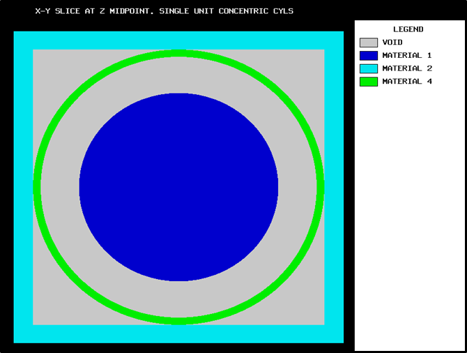
Fig. 8.1.71 Mixture color plot for single unit with centered origin.

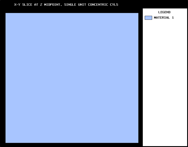
Fig. 8.1.72 Unit map color plot for single unit with centered origin.

Example 8.1.19 Associated data for single unit mixture map.

 mixture map

 mixture  0 1 2 4
  symbol    1 2 3
       upper  left          lower right
       coordinates          coordinates
 x     -4.6000e+00           4.6000e+00
 y      4.6000e+00          -4.6000e+00
 z      0.0000e+00           0.0000e+00

           u axis      v axis
           (down)      (across)
 x         0.00000      1.00000
 y        -1.00000      0.00000
 z         0.00000      0.00000

 nu=  640   nv=  640     delu= 1.4375e-02     delv= 1.4375e-02     lpi=  10.000

Example 8.1.20 Associated data for single unit map.

 x-y slice at z midpoint. single unit concentric cyls

unit map

    unit  1
  symbol  1
       upper  left          lower right
       coordinates          coordinates
 x     -4.6000e+00           4.6000e+00
 y      4.6000e+00          -4.6000e+00
 z      0.0000e+00           0.0000e+00
           u axis      v axis
           (down)      (across)
 x         0.00000      1.00000
 y        -1.00000      0.00000
 z         0.00000      0.00000
 nu=  640   nv=  640     delu= 1.4375e-02     delv= 1.4375e-02     lpi=  10.000

EXAMPLE 2. SINGLE UNIT WITH OFFSET ORIGIN.

The physical problem is the same as that described in Example 1: two concentric cylinders in a cuboid. The dimensions are exactly the same, and the difference is in the choice of the origin. In this geometry description, the origin was specified as the most negative point of the unit. Thus, the cylinders must have an origin specified to center them in the cuboid, and the cuboid extends from 0.0 to 8.6 in X and Y and from 0.0 to 32 in Z as shown in the problem description below.

KENO V.a:

=KENO5
SINGLE UNIT CONCENTRIC CYLINDERS IN CUBOID WITH ORIGIN AT CORNER
READ PARAM  RUN=NO LIB=41 END PARAM
READ MIXT  SCT=1  MIX=1 92500 4.7048-2 MIX=2 200 1.0 MIX=3 502 0.1
MIX=4 200 1.0
END MIXT
READ GEOM
UNIT 1
CYLINDER 1 1 2.6 31.0 1.0 ORIGIN 4.3 4.3
CYLINDER 0 1 3.6 31.0 1.0 ORIGIN 4.3 4.3
CYLINDER 4 1 3.8 31.0 1.0 ORIGIN 4.3 4.3
CUBOID 0 1 8.1 0.5 8.1 0.5 31.0 1.0
CUBOID 2 1 8.6 0.0 8.6 0.0 32.0 0.0
END GEOM
READ PLOT
TTL='X-Y SLICE AT Z MIDPOINT. SINGLE UNIT CONCENTRIC CYLS.'
XUL=-0.3 YUL=8.9 ZUL=16.0 XLR=8.9 YLR=-0.3 ZLR=16.0
UAX=1.0 VDN=-1.0 NAX=640 END
PIC=UNIT  END
END PLOT
END DATA
END

KENO-VI:

=KENOVI
SINGLE UNIT CONCENTRIC CYLINDERS IN CUBOID WITH ORIGIN AT CORNER
READ PARAM  RUN=NO LIB=41 TME=0.5 END PARAM
READ MIXT  SCT=1  MIX=1 92500 4.7048-2 MIX=2 200 1.0 MIX=3 502 0.1
MIX=4 200 1.0
END MIXT
READ GEOM
GLOBAL UNIT 1
CYLINDER 1 2.6 31.0 1.0 ORIGIN X=4.3 Y=4.3
CYLINDER 2 3.6 31.0 1.0 ORIGIN X=4.3 Y=4.3
CYLINDER 3 3.8 31.0 1.0 ORIGIN X=4.3 Y=4.3
CUBOID  4 8.1 0.5 8.1 0.5 31.0 1.0
CUBOID 5  8.6 0.0 8.6 0.0 32.0 0.0
MEDIA 1 1 1
MEDIA 0 1 2 -1
MEDIA 4 1 3  -2 -1
MEDIA 0 1 4 -3 -2 -1
MEDIA 2 1 5 -4
BOUNDARY  5
END GEOM
READ PLOT
TTL='X-Y SLICE AT Z MIDPOINT. SINGLE UNIT CONCENTRIC CYLS.'
XUL=-0.3  YUL=8.9  ZUL=16.0  XLR=8.9  YLR=-0.3  ZLR=16.0
UAX=1.0  VDN=-1.0  NAX=640 END
PIC=UNIT NCH='01' END
END PLOT
END DATA
END

The plot data included above will draw a mixture map of an X-Y slice taken at the half height (Z = 16.0). It will also draw a unit map of the same slice. The plot dimensions extend 0.3 cm beyond the problem dimensions to provide a black border around the plot. The associated plot data specification for the mixture map is shown in Example 8.1.21, the mixture map is shown in Fig. 8.1.73, and the associated plot data for the unit map is shown in Example 8.1.22. The unit map is identical to Fig. 8.1.72 and is not included.

Example 8.1.21 Associated data for mixture map of single unit with offset origin.

x-y slice at z midpoint. single unit concentric cyls.

mixture map

 mixture  0 1 2 4
  symbol    1 2 3
       upper  left          lower right
       coordinates          coordinates
 x     -3.0000e-01           8.9000e+00
 y      8.9000e+00          -3.0000e-01
 z      1.6000e+01           1.6000e+01
           u axis      v axis
           (down)      (across)
 x         0.00000      1.00000
 y        -1.00000      0.00000
 z         0.00000      0.00000
 nu=  640   nv=  640     delu= 1.4375e-02     delv= 1.4375e-02     lpi=  10.000

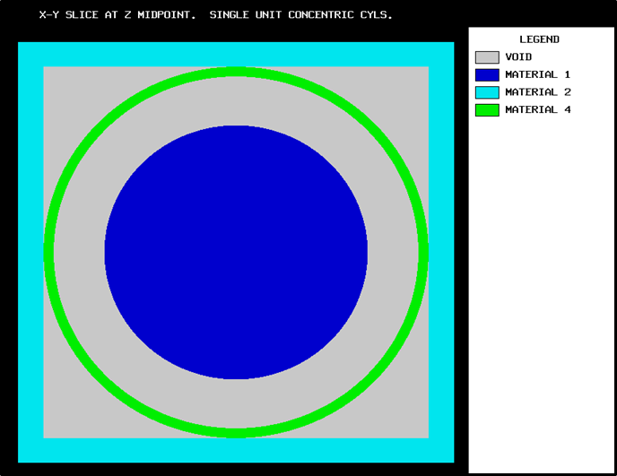
Fig. 8.1.73 Mixture map of single unit with offset origin.

Example 8.1.22 Associated data for unit map of single unit with offset origin.

 x-y slice at z midpoint. single unit concentric cyls.

unit map

    unit  1
  symbol  1
       upper  left          lower right
       coordinates          coordinates
 x     -3.0000e-01           8.9000e+00
 y      8.9000e+00          -3.0000e-01
 z      1.6000e+01           1.6000e+01
           u axis      v axis
           (down)      (across)
 x         0.00000      1.00000
 y        -1.00000      0.00000
 z         0.00000      0.00000
 nu=  640   nv=  640     delu= 1.4375e-02     delv= 1.4375e-02     lpi=  10.000

EXAMPLE 3. A 2 \(\times\) 2 \(\times\) 2 UNREFLECTED ARRAY OF CONCENTRIC CYLINDERS IN CUBOIDS

The physical representation of this example is a 2 \(\times\) 2 \(\times\) 2 array of the configuration described in Example 1 of this section. The input data description for this array is given below:

KENO V.a:

=KENOVA
2x2x2 BARE ARRAY OF CONCENTRIC CYLINDERS IN CUBOID
READ PARAM  RUN=NO LIB=41 END PARAM
READ MIXT  SCT=1  MIX=1 92500 4.7048-2 MIX=2 200 1.0 MIX=3 502 0.1
MIX=4 200 1.0
END MIXT
READ GEOM
UNIT 1
CYLINDER 1 1 2.6 2P15.0
CYLINDER 0 1 3.6 2P15.0
CYLINDER 4 1 3.8 2P15.0
CUBOID 0 1 4P3.8 2P15.0
CUBOID 2 1 4P4.3 2P16.0
END GEOM
READ ARRAY NUX=2 NUY=2 NUZ=2 END ARRAY
READ PLOT
TTL='X-Y SLICE AT HALF HEIGHT OF BOTTOM LAYER.'
XUL=-0.3 YUL=17.5 ZUL=16.0 XLR=17.5 YLR=-0.3 ZLR=16.0
UAX=1.0 VDN=-1.0 NAX=640  END
TTL='X-Z SLICE THROUGH FRONT ROW, Y=12.9.'
XUL=-1.0 YUL=12.9 ZUL=65.0 XLR=18.2 YLR=12.9 ZLR=-1.0
UAX=1.0 WDN=-1.0 NAX=320 END
END PLOT
END DATA
END

KENO-VI:

=KENOVI
2x2x2 BARE ARRAY OF CONCENTRIC CYLINDERS IN CUBOID
READ PARAM  RUN=NO LIB=41 TME=8.5 END PARAM
READ MIXT  SCT=1  MIX=1 92500 4.7048-2 MIX=2 200 1.0 MIX=3 502 0.1
MIX=4 200 1.0
END MIXT
READ GEOM
UNIT 1
CYLINDER 1 2.6 2P15.0
CYLINDER 2 3.6 2P15.0
CYLINDER 3 3.8 2P15.0
CUBOID 4 4P3.8 2P15.0
CUBOID 5 4P4.3 2P16.0
MEDIA 1 1 1
MEDIA 0 1 2 -1
MEDIA 4 1 3 -2 -1
MEDIA 0 1 4 -3 -2 -1
MEDIA  2 1 -5 -4
BOUNDARY  5
GLOBAL UNIT 2
CUBOID 1 17.2 0.0 17.2 0.0 64.0 0.0
ARRAY 1 1 PLACE 1 1 1 4.3 4.3 16.0
BOUNDARY  1
END GEOM
READ ARRAY  ARA=1 NUX=2 NUY=2 NUZ=2 FILL F1 END FILL  END ARRAY

READ PLOT
TTL='X-Y SLICE AT HALF HEIGHT OF BOTTOM LAYER.'
XUL=-0.3 YUL=17.5 ZUL=16.0 XLR=17.5 YLR=-0.3 ZLR=16.0
UAX=1.0 VDN=-1.0 NAX=640 END
TTL='X-Z SLICE THROUGH FRONT ROW, Y=12.9.'
XUL=-1.0 YUL=12.9 ZUL=65.0 XLR=18.2 YLR=12.9 ZLR=-1.0
UAX=1.0 WDN=-1.0 NAX=320 END
END PLOT
END DATA
END

As stated at the beginning of Sect. 8.1.4.10, the origin of a plot is defined as the origin of the GLOBAL UNIT. Each individual unit in the array is 8.6 cm wide in X and Y and 32 cm high in Z. Since the array has two units stacked in each direction, the array is 17.2 cm wide in X and Y and is 64 cm high. Therefore, the array exists from X = 0.0 to X = 17.2, from Y = 0.0 to Y = 17.2 and from Z = 0.0 to Z = 64.0.

The first color plot is to generate an X-Y slice through the array at the half height (Z = 16.0 cm) of the first layer as shown in Fig. 8.1.74. It is desirable to create an image with a larger extent than the global unit to ensure that the boundaries are as expected. This is achieved by setting the boundaries of the plot larger than the array. In this case, the boundaries were arbitrarily set 0.3 cm larger than the array, resulting in a black border around the array. If the plot were to exclude everything external to the array, the following coordinates could have been entered: XUL=0.0 YUL=17.2 ZUL=16.0 XLR=17.2 YLR=0.0 ZLR=16.0. This would have eliminated the black border. The existing plot was made using XUL= -0.3 YUL=17.5 ZUL=16.0 XLR=17.5 YLR= -0.3 ZLR=16.0.

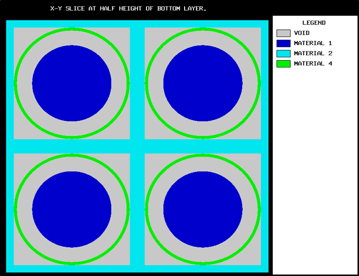
Fig. 8.1.74 X-Y plot of 2 \(\times\) 2 \(\times\) 2 bare array.

The second color plot is to generate an X-Z slice through the center of the front row of the array. In order to obtain a black border, the coordinates of X and Z were arbitrarily set 1.0 cm larger than the boundaries of the array. The center of the front row occurs at Y = 12.9. The coordinates of the plot were: XUL= -1.0 ZUL=65.0 YUL=12.9 XLR=18.2 ZLR= -1.0 YLR=12.9. The resulting mixture map is shown in Fig. 8.1.75.

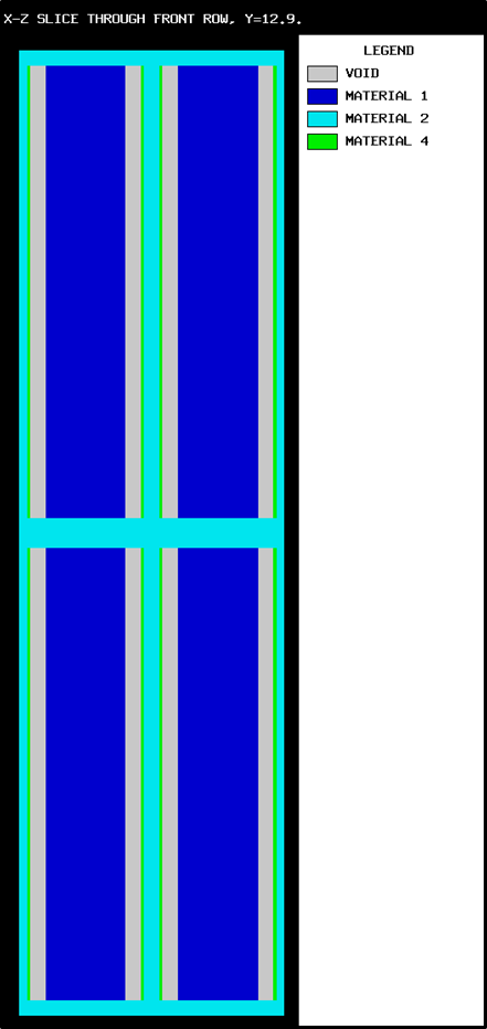
Fig. 8.1.75 X-Z plot of 2 \(\times\) 2 \(\times\) 2 bare array.

EXAMPLE 4. A 2 \(\times\) 2 \(\times\) 2 REFLECTED ARRAY WITH THE ORIGIN AT THE MOST NEGATIVE POINT OF THE ARRAY

The ARRAY is described in Example 3 of this section with a 6 in. concrete reflector on all faces. The input data description for this array is given below.

KENO V.a:

=KENOVA
2x2x2 REFLECTED ARRAY OF CONCENTRIC CYLINDERS IN CUBOID
READ PARAM  RUN=NO LIB=41 END PARAM
READ MIXT  SCT=1  MIX=1 92500 4.7048-2 MIX=2 200 1.0 MIX=3 301 1.0
MIX=4 200 1.0
END MIXT
READ GEOM
UNIT 1
CYLINDER 1 1 2.6 2P15.0
CYLINDER 0 1 3.6 2P15.0
CYLINDER 4 1 3.8 2P15.0
CUBOID 0 1 4P3.8 2P15.0
CUBOID 2 1 4P4.3 2P16.0
GLOBAL
UNIT 2
ARRAY 1  3*0.0
REFLECTOR 3 2 6*5.0 3
REFLECTOR 3 5 6*0.24 1
END GEOM
READ BIAS ID=301 2 5 END BIAS
READ ARRAY ARA=1 NUX=2 NUY=2 NUZ=2 FILL F1 END FILL END ARRAY
READ PLOT
TTL='X-Y SLICE AT HALF HEIGHT OF BOTTOM LAYER.INCLUDES REFL.'
XUL=-16.24 YUL=33.44 ZUL=16.0 XLR=33.44 YLR=-16.24 ZLR=16.0
UAX=1.0 VDN=-1.0 NAX=640  END
TTL='X-Y SLICE AT HALF HEIGHT OF BOTTOM LAYER, INCLUDE 3 CM OF REFL.'
XUL=-3.0 YUL=20.2 ZUL=16.0 XLR=20.2 YLR=-3.0 ZLR=16.0
UAX=1.0 VDN=-1.0 NAX=640 END
TTL='X-Z SLICE THROUGH FRONT ROW, Y=12.9. INCLUDE REFLECTOR'
XUL=-16.24 YUL=12.9 ZUL=80.24 XLR=33.44 YLR=12.9 ZLR=-16.24
UAX=1.0 WDN=-1.0 NAX=640 END
TTL='X-Z SLICE THROUGH FRONT ROW, Y=12.9. INCLUDE 3 CM OF REFLECTOR'
XUL=-3.0 YUL=12.9 ZUL=67.0 XLR=20.2 YLR=12.9 ZLR=-3.0
UAX=1.0 WDN=-1.0 NAX=640 END
END PLOT
END DATA
END

KENO-VI:

=KENOVI
2x2x2 REFLECTED ARRAY OF CONCENTRIC CYLINDERS IN CUBOID
READ PARAM  RUN=NO LIB=41 TME=0.5 END PARAM
READ MIXT  SCT=1  MIX=1 92500 4.7048-2 MIX=2 200 1.0 MIX=3 301 1.0
MIX=4 200 1.0
END MIXT
READ GEOM
UNIT 1
CYLINDER 1 2.6 2P15.0
CYLINDER 2 3.6 2P15.0
CYLINDER 3 3.8 2P15.0
CUBOID 4  4P3.8 2P15.0
CUBOID 5  4P4.3 2P16.0
MEDIA 1 1 1
MEDIA 0 1 2 -1
MEDIA 4 1 3 -2
MEDIA 0 1 4 -3
MEDIA 2 1 5 -4
BOUNDARY  5
GLOBAL UNIT 2
CUBOID 1  17.2       0.0    17.2       0.0    64.0        0.0
CUBOID 2  22.20    -5.00  22.20    -5.00  69.00     -5.00
CUBOID 3  27.20  -10.00  27.20  -10.00  74.00   -10.00
CUBOID 4  32.20  -15.00  32.20  -15.00  79.00   -15.00
CUBOID 5  32.44  -15.24  32.44  -15.24  79.24   -15.24
ARRAY 1  1  PLACE 1 1 1 4.3 4.3 16.0
MEDIA 3  2  2  -1
MEDIA 3  3  3  -2
MEDIA 3  4  4  -3
MEDIA 3  5  5  -4
BOUNDARY  5
END GEOM
READ BIAS ID=301 2 5 END BIAS
READ ARRAY  ARA=1  NUX=2  NUY=2  NUZ=2  FILL F1  END FILL   END ARRAY
READ PLOT
TTL='X-Y SLICE AT HALF HEIGHT OF BOTTOM LAYER.INCLUDES REFL.'
XUL=-16.24  YUL=33.44  ZUL=16.0  XLR=33.44  YLR=-16.24  ZLR=16.0
UAX=1.0  VDN=-1.0  NAX=640  END
TTL='X-Y SLICE AT HALF HEIGHT OF BOTTOM LAYER, INCLUDE 3 CM OF REFL.'
XUL=-3.0  YUL=20.2  ZUL=16.0  XLR=20.2  YLR=-3.0  ZLR=16.0
UAX=1.0  VDN=-1.0  NAX=640  END
TTL='X-Z SLICE THROUGH FRONT ROW, Y=12.9. INCLUDE REFLECTOR'
XUL=-16.24  YUL=12.9  ZUL=80.24  XLR=33.44  YLR=12.9  ZLR=-16.24
UAX=1.0  WDN=-1.0  NAX=640  END
TTL='X-Z SLICE THROUGH FRONT ROW, Y=12.9. INCLUDE 3 CM OF REFLECTOR'
XUL=-3.0  YUL=12.9  ZUL=67.0  XLR=20.2  YLR=12.9  ZLR=-3.0
UAX=1.0  WDN=-1.0  NAX=640  END
END PLOT
END DATA
END

The ARRAY record specifies the array number and the coordinates of the most negative point of the array to be (0.0,0.0,0.0) and the coordinates of the most positive point to be (17.2,17.2,64.0). Thus the reflected array extends from -15.24 cm to +32.44 cm in X and Y and from -15.24 to +79.24 in Z.

The first color plot for this example is to show an X-Y slice through the array and reflector at the half height of the bottom layer. A black border is used to verify that the entire reflector has been shown. This is accomplished by arbitrarily setting the plot boundaries 1 cm beyond the reflector boundaries. The coordinates used for this plot are XUL = -16.24 YUL = 33.44 ZUL = 16.0 XLR = 33.44 YLR = 16.24 ZLR = 16.0. The plot data description is shown in Example 8.1.23, and the plot is shown in Fig. 8.1.76.

Example 8.1.23 Plot data for X-Y slice of Example 4.

x-y slice at half height of bottom layer. includes refl.

mixture map

 mixture  0 1 2 3 4
  symbol    1 2 3 4
       upper  left          lower right
       coordinates          coordinates
 x     -1.6240e+01           3.3440e+01
 y      3.3440e+01          -1.6240e+01
 z      1.6000e+01           1.6000e+01
           u axis      v axis
           (down)      (across)
 x         0.00000      1.00000
 y        -1.00000      0.00000
 z         0.00000      0.00000
 nu=  640   nv=  640     delu= 7.7625e-02     delv= 7.7625e-02     lpi=  10.000

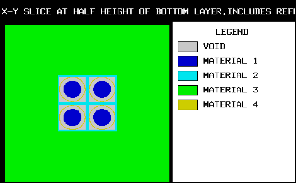
Fig. 8.1.76 X-Y plot of 2 \(\times\) 2 \(\times\) 2 reflected array.

The next color plot is the same as the previous plot, except this plot includes only the first 3 cm of the reflector in order to show more detail. The coordinates used for this plot are XUL= -3.0 YUL=20.2 ZUL=16.0 XLR=20.2 YLR= -3.0 ZLR=16.0. This plot data description is given in Example 8.1.24, and the plot is shown in Fig. 8.1.77.

Example 8.1.24 Plot data for enlarged X-Y slice of Example 4.

x-y slice at half height of bottom layer, include 3 cm of refl.
mixture map

 mixture  0 1 2 3 4
  symbol    1 2 3 4
       upper  left          lower right
       coordinates          coordinates
 x     -3.0000e+00           2.0200e+01
 y      2.0200e+01          -3.0000e+00
 z      1.6000e+01           1.6000e+01
           u axis      v axis
           (down)      (across)
 x         0.00000      1.00000
 y        -1.00000      0.00000
 z         0.00000      0.00000
 nu=  640   nv=  640     delu= 3.6250e-02     delv= 3.6250e-02     lpi=  10.000

Fig. 8.1.77 Enlarged X-Y plot of 2 \(\times\) 2 \(\times\) 2 reflected array.

The third color plot for this example is an X-Z slice through the center of the front row. An extra 1 cm is included in the coordinates to provide a black border around the plot. The coordinates are: XUL= -16.24 YUL=12.9 ZUL=80.24 XLR=33.44 YLR=12.9 ZLR= -16.24. The resultant plot data and plot are shown in Example 8.1.25 and Fig. 8.1.78. X-Z plot for 2 \(\times\) 2 \(\times\) 2 reflected array.

Example 8.1.25 Plot data for X-Z slice of Example 4.

x-z slice through front row, y=12.9. include reflector

mixture map

 mixture  0 1 2 3 4
  symbol    1 2 3 4
       upper  left          lower right
       coordinates          coordinates
 x     -1.6240e+01           3.3440e+01
 y      1.2900e+01           1.2900e+01
 z      8.0240e+01          -1.6240e+01
           u axis      v axis
           (down)      (across)
 x         0.00000      1.00000
 y         0.00000      0.00000
 z        -1.00000      0.00000
 nu= 1242   nv=  640     delu= 7.7625e-02     delv= 7.7625e-02     lpi=  10.000

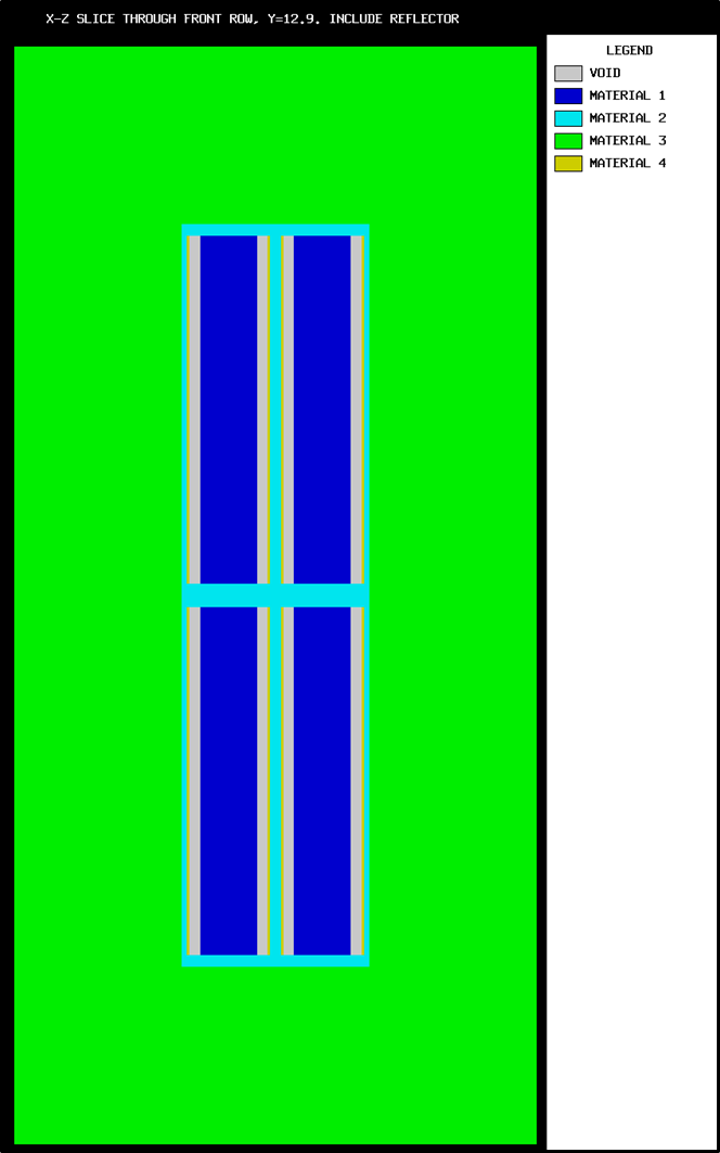
Fig. 8.1.78 X-Z plot for 2 \(\times\) 2 \(\times\) 2 reflected array.

The last color plot for this example is the same as the previous one, except only 3 cm of the reflector is included in the plot. The plot data and associated plot are shown in Example 8.1.26 and Fig. 8.1.79.

Example 8.1.26 Plot data for enlarged X-Z slice of Example 4.

x-z slice through front row, y=12.9. include 3 cm of reflector

mixture map

 mixture  0 1 2 3 4
  symbol    1 2 3 4
       upper  left          lower right
       coordinates          coordinates
 x     -3.0000e+00           2.0200e+01
 y      1.2900e+01           1.2900e+01
 z      6.7000e+01          -3.0000e+00
           u axis      v axis
           (down)      (across)
 x         0.00000      1.00000
 y         0.00000      0.00000
 z        -1.00000      0.00000
 nu= 1931   nv=  640     delu= 3.6250e-02     delv= 3.6250e-02     lpi=  10.000

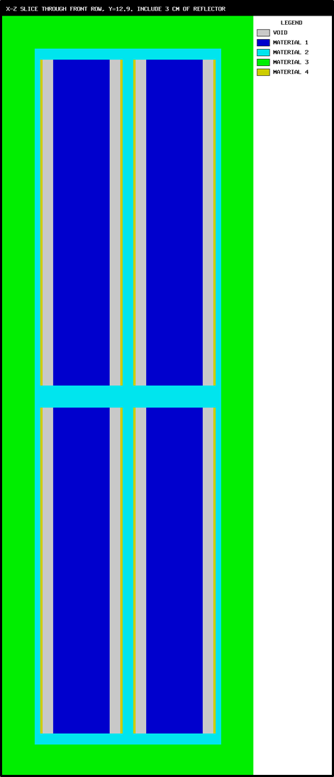
Fig. 8.1.79 Enlarged X-Z plot of 2 \(\times\) 2 \(\times\) 2 reflected array.

EXAMPLE 5. A 2 \(\times\) 2 \(\times\) 2 REFLECTED ARRAY WITH THE ORIGIN CENTERED IN THE ARRAY

This example is physically identical to Example 4. The difference is in the specification of the origin. The bare array is 17.2 cm wide in X and Y and 64 cm high. The origin (0,0,0) can be placed at the exact center of the array by specifying the most negative point of the array as X = -8.6, Y = -8.6 and Z = -32.0. This is done using the ARRAY description in the geometry block. Because the origin is located at a different position, the coordinates of the plots will also be different. The input data description for this example is given below.

KENO V.a:

=KENOVA
2x2x2 REFLECTED ARRAY OF CONCENTRIC CYLINDERS IN CUBOID
READ PARAM  RUN=NO LIB=41 TME=0.5 END PARAM
READ MIXT  SCT=1  MIX=1 92500 4.7048-2 MIX=2 200 1.0 MIX=3 301 1.0
MIX=4 200 1.0
END MIXT
READ GEOM
UNIT 1
CYLINDER 1 1 2.6 2P15.0
CYLINDER 0 1 3.6 2P15.0
CYLINDER 4 1 3.8 2P15.0
CUBOID 0 1 4P3.8 2P15.0
CUBOID 2 1 4P4.3 2P16.0
GLOBAL
UNIT 2
ARRAY 1 1 2*-8.6 -32.0
REFLECTOR 3 2 6*5.0 3
REFLECTOR 3 5 6*0.24 1
END GEOM
READ BIAS ID=301 2 5 END BIAS
READ ARRAY ARA=1 NUX=2 NUY=2 NUZ=2 FILL F1 END FILL  END ARRAY
READ PLOT
TTL='X-Y SLICE AT HALF HEIGHT OF BOTTOM LAYER.INCLUDES REFL.'
XUL=-24.84 YUL=24.84 ZUL=-8.0 XLR=24.84 YLR=-24.84 ZLR=-8.0
UAX=1.0 VDN=-1.0 NAX=640  END
TTL='X-Y SLICE AT HALF HEIGHT OF BOTTOM LAYER, INCLUDE 3 CM OF REFL.'
XUL=-11.6 YUL=11.6 ZUL=-8.0 XLR=11.6 YLR=-11.6 ZLR=-8.0
UAX=1.0 VDN=-1.0 NAX=640  END
TTL='X-Z SLICE THROUGH FRONT ROW. Y=4.3  INCLUDE REFLECTOR'
XUL=-24.84 YUL=4.3 ZUL=48.24 XLR=24.84 YLR=4.3 ZLR=-48.24
UAX=1.0 WDN=-1.0 NAX=640 END
TTL='X-Z SLICE THROUGH FRONT ROW, Y=4.3  INCLUDE 3 CM OF REFLECTOR'
XUL=-11.6 YUL=4.3 ZUL=35.0 XLR=11.6 YLR=4.3 ZLR=-35.0
UAX=1.0 WDN=-1.0 NAX=640 END
END PLOT
END DATA
END

KENO-VI:

=KENOVI
2x2x2 REFLECTED ARRAY OF CONCENTRIC CYLINDERS IN CUBOID
READ PARAM  RUN=NO LIB=41 TME=0.5 END PARAM
READ MIXT  SCT=1  MIX=1 92500 4.7048-2 MIX=2 200 1.0 MIX=3 301 1.0
MIX=4 200 1.0
END MIXT
READ GEOM
UNIT 1
CYLINDER 1 2.6 2P15.0
CYLINDER 2 3.6 2P15.0
CYLINDER 3 3.8 2P15.0
CUBOID 4 4P3.8 2P15.0
CUBOID 5 4P4.3 2P16.0
MEDIA 1 1
MEDIA 0 1 2 -1
MEDIA 4 1 3 -2
MEDIA 0 1 4 -3
MEDIA 2 1 5 -4
BOUNDARY  5
GLOBAL UNIT 2
CUBOID 1 8.6 -8.6 8.6 -8.6 32.0 -32.0
CUBOID 2 13.6 -13.6 13.6 -13.6 37.0 -37.0
CUBOID 3 18.6 -18.6 18.6 -18.6 42.0 -42.0
CUBOID 4 23.6 -23.6 23.6 -23.6 47.0 -47.0
CUBOID 5 23.84 -23.84 23.84 -23.84 47.24 -47.24
ARRAY 1 1 PLACE 1 1 1 -4.3 -4.3 -16.0
MEDIA 3 2 2 -1
MEDIA 3 3 3 -2
MEDIA 3 4 4 -3
MEDIA 3 5 5 -4
BOUNDARY  5
END GEOM
READ BIAS ID=301 2 5 END BIAS
READ ARRAY ARA=1 NUX=2 NUY=2 NUZ=2I FILL F1 END FILL   END ARRAY
READ PLOT
TTL='X-Y SLICE AT HALF HEIGHT OF BOTTOM LAYER INCLUDES REFL.'
XUL=-24.84 YUL=24.84 ZUL=-8.0 XLR=24.84 YLR=-24.84 ZLR=-8.0
UAX=1.0  VDN=-1.0  NAX=130  NCH=' *=.X'  END
TTL='X-Y SLICE AT HALF HEIGHT OF BOTTOM LAYER, INCLUDE 3 CM OF REFL.'
XUL=-11.6  YUL=11.6  ZUL=-8.0  XLR=11.6  YLR=-11.6  ZLR=-8.0
UAX=1.0  VDN=-1.0  NAX=640  END
TTL='X-Z SLICE THROUGH FRONT ROW. Y=4.3  INCLUDE REFLECTOR'
XUL=-24.84  YUL=4.3  ZUL=48.24  XLR=24.84  YLR=4.3  ZLR=-48.24
UAX=1.0  WDN=-1.0  NAX=640 END
TTL='X-Z SLICE THROUGH FRONT ROW, Y=4.3  INCLUDE 3 CM OF REFLECTOR'
XUL=-11.6  YUL=4.3  ZUL=35.0  XLR=11.6  YLR=4.3  ZLR=-35.0
UAX=1.0  WDN=-1.0  NAX=640  END
END PLOT
END DATA
END

The first color plot for this example covers exactly the same area as the first plot for Example 4. The plot data and the plot are given in Example 8.1.27 and Fig. 8.1.80, respectively.

Example 8.1.27 Plot data for X-Y slice of Example 5.

x-y slice at half height of bottom layer.includes refl.
mixture map

 mixture  0 1 2 3 4
  symbol    1 2 3 4
       upper  left          lower right
       coordinates          coordinates
 x     -2.4840e+01           2.4840e+01
 y      2.4840e+01          -2.4840e+01
 z     -8.0000e+00          -8.0000e+00
           u axis      v axis
           (down)      (across)
 x         0.00000      1.00000
 y        -1.00000      0.00000
 z         0.00000      0.00000
 nu=  640   nv=  640     delu= 7.7625e-02     delv= 7.7625e-02     lpi=  10.000

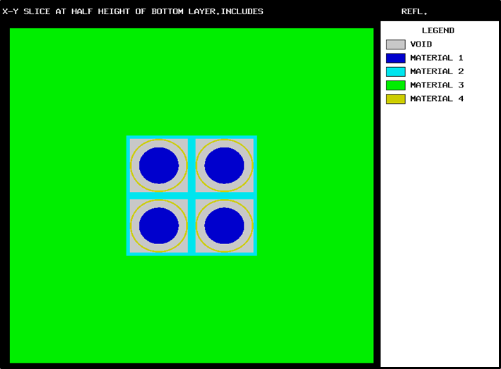
Fig. 8.1.80 X-Y plot of 2 \(\times\) 2 \(\times\) 2 reflected array with centered origin.

The Example 5 plot data and associated plots for an enlarged X-Y plot, an X-Z plot and an enlarged X-Z plot are given in Example 8.1.28 through Fig. 8.1.83.

Example 8.1.28 Plot data for an enlarged X-Y slice of Example 5.

x-y slice at half height of bottom layer, include 3 cm of refl.

mixture map

 mixture  0 1 2 3 4
  symbol    1 2 3 4
       upper  left          lower right
       coordinates          coordinates
 x     -1.1600e+01           1.1600e+01
 y      1.1600e+01          -1.1600e+01
 z     -8.0000e+00          -8.0000e+00
           u axis      v axis
           (down)      (across)
 x         0.00000      1.00000
 y        -1.00000      0.00000
 z         0.00000      0.00000
 nu=  640   nv=  640     delu= 3.6250e-02     delv= 3.6250e-02     lpi=  10.000

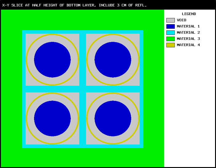
Fig. 8.1.81 Enlarged X-Y plot of 2 \(\times\) 2 \(\times\) 2 reflected array with centered origin.

Example 8.1.29 Plot data for X-Z slice of Example 5.

x-z slice through front row. y=4.3  include reflector

mixture map

 mixture  0 1 2 3 4
  symbol    1 2 3 4
       upper  left          lower right
       coordinates          coordinates
 x     -2.4840e+01           2.4840e+01
 y      4.3000e+00           4.3000e+00
 z      4.8240e+01          -4.8240e+01
           u axis      v axis
           (down)      (across)
 x         0.00000      1.00000
 y         0.00000      0.00000
 z        -1.00000      0.00000
 nu= 1242   nv=  640     delu= 7.7625e-02     delv= 7.7625e-02     lpi=  10.000

Fig. 8.1.82 X-Z plot of reflected 2 \(\times\) 2 \(\times\) 2 array with centered origin.

Example 8.1.30 Plot data for enlarged X-Z slice of Example 5.

x-z slice through front row, y=4.3  include 3 cm of reflector

mixture map

 mixture  0 1 2 3 4
  symbol    1 2 3 4
       upper  left          lower right
       coordinates          coordinates
 x     -1.1600e+01           1.1600e+01
 y      4.3000e+00           4.3000e+00
 z      3.5000e+01          -3.5000e+01
           u axis      v axis
           (down)      (across)
 x         0.00000      1.00000
 y         0.00000      0.00000
 z        -1.00000      0.00000
 nu= 1931   nv=  640     delu= 3.6250e-02     delv= 3.6250e-02     lpi=  10.000

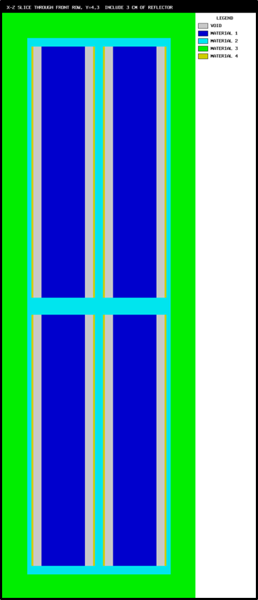
Fig. 8.1.83 Enlarged X-Z plot of reflected 2 \(\times\) 2 \(\times\) 2 array with centered origin.

EXAMPLE 6. NESTED HOLES.

The nested hole description is provided in Sect. 8.1.4.6.2. Because this example involves a complicated placement of units, it is helpful useful to the user to generate a mixture plot and/or a unit plot for the problem. The resultant mixture plot for this problem is shown in Fig. 8.1.84, and the data description for Example 6 follows.

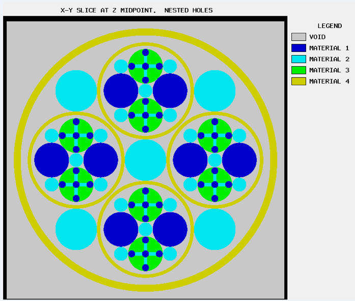
Fig. 8.1.84 Mixture plot of nested holes problem.

Example 8.1.31 Plot data for unit plot of nested holes.

x-y slice at z midpoint. nested holes. unit map
0                                        unit map
    unit  1 2 3 4 5 6 7 8 9
  symbol  1 2 3 4 5 6 7 8 9

       overall system coordinates:
       xmin= 0.00000e+00   xmax= 8.00000e+00   ymin= 0.00000e+00   ymax= 8.00000e+00
       zmin= 0.00000e+00   zmax= 3.20000e+01
       upper  left          lower right
       coordinates          coordinates
 x     -1.0000e-01           8.1000e+00
 y      8.1000e+00          -1.0000e-01
 z      1.6000e+01           1.6000e+01
           u axis      v axis
           (down)      (across)
 x         0.00000      1.00000
 y        -1.00000      0.00000
 z         0.00000      0.00000
 nu=  640   nv=  640     delu= 1.2813e-02     delv= 1.2813e-02     lpi=  10.000

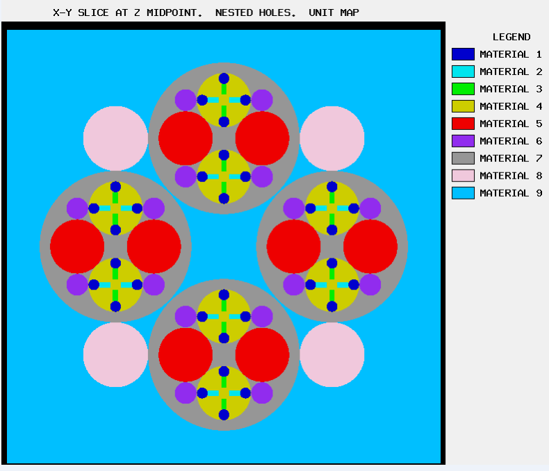
Fig. 8.1.85 Unit plot of nested holes problem.

KENO V.a:

=KENOVA
NESTED HOLES SAMPLE
READ PARAM  RUN=NO LIB=41  END PARAM
READ MIXT  SCT=1  MIX=1 92500 4.7048-2 MIX=2 200 1.0 MIX=3 502 0.1
MIX=4 200 1.0
END MIXT
READ GEOM
UNIT 1
CYLINDER 1 1 0.1 2P15.0
UNIT 2
CUBOID 2 1 2P0.1 2P0.05 2P15.0
UNIT 3
CUBOID 2 1 2P0.05 2P0.1 2P15.0
UNIT 4
CYLINDER 1 1 0.1 2P15.0
CYLINDER 3 1 0.5 2P15.0
HOLE 1  0.0 -0.4 0.0
HOLE 1  0.4  0.0 0.0
HOLE 1  0.0  0.4 0.0
HOLE 1 -0.4  0.0 0.0
HOLE 2 -0.2  0.0 0.0
HOLE 2  0.2  0.0 0.0
HOLE 3  0.0 -0.2 0.0
HOLE 3  0.0  0.2 0.0
UNIT 5
CYLINDER 1 1 0.5 2P15.0
UNIT 6
CYLINDER 2 1 0.2 2P15.0
UNIT 7
CYLINDER 2 1 0.2 2P15.0
CYLINDER 0 1 1.3 2P15.0
HOLE 5 0.707107 2*0.0
HOLE 6 0.707107 0.707107 0.0
HOLE 4 0.0 0.707107 0.0
HOLE 6 -0.707107 0.707107 0.0
HOLE 5 -0.707107 0.0 0.0
HOLE 6 -0.707107 -0.707107 0.0
HOLE 4 0.0 -0.707107 0.0
HOLE 6 0.707107 -0.707107 0.0
CYLINDER 4 1 1.4 2P15.0
UNIT 8
CYLINDER 2 1 0.6 2P15.0
UNIT 9
CYLINDER 2 1 0.6 2P15.0
CYLINDER 0 1 3.6 2P15.0
HOLE 7 2.0 0.0 0.0
HOLE 8 2*2.0 0.0
HOLE 7 0.0 2.0 0.0
HOLE 8 -2.0 2.0 0.0
HOLE 7 -2.0 2*0.0
HOLE 8 2*-2.0 0.0
HOLE 7 0.0 -2.0 0.0
HOLE 8 2P2.0 0.0
CYLINDER 4 1 3.8 2P15.0
CUBOID 0 1 4P4.0 2P16.0
END GEOM
READ ARRAY ARA=1 NUX=1 NUY=1 NUZ=1  FILL 9 END ARRAY
READ PLOT
TTL='X-Y SLICE AT Z MIDPOINT. NESTED HOLES'
XUL=-0.1 YUL=8.1 ZUL=16.0 XLR=8.1 YLR=-0.1 ZLR=16
UAX=1.0 VDN=-1.0 NAX=640  END
TTL='X-Y SLICE AT Z MIDPOINT. NESTED HOLES. UNIT MAP'
PIC=UNIT  END
END PLOT
END DATA
END

KENO-VI:

=KENOVI
NESTED HOLES SAMPLE
READ PARAM  RUN=NO LIB=41 TME=0.5 END PARAM
READ MIXT  SCT=1  MIX=1 92500 4.7048-2 MIX=2 200 1.0 MIX=3 502 0.1
MIX=4 200 1.0
END MIXT
READ GEOM
UNIT 1
CYLINDER 1 0.1 2P15.0
CYLINDER 2 0.1 2P15.0 ORIGIN Y=-0.4
CYLINDER 3 0.1 2P15.0 ORIGIN X=0.4
CYLINDER 4 0.1 2P15.0 ORIGIN Y=0.4
CYLINDER 5 0.1 2P15.0 ORIGIN X=-0.4
CUBOID 6 2P0.1 2P0.05 2P15.0 ORIGIN X=-0.2
CUBOID 7 2P0.1 2P0.05 2P15.0 ORIGIN X=0.2
CUBOID 8 2P0.05 2P0.1 2P15.0 ORIGIN Y=-0.2
CUBOID 9 2P0.05 2P0.1 2P15.0 ORIGIN Y=0.2
CYLINDER 10 0.5 2P15.0
MEDIA 1 1 1 -6 -7 -8 -9
MEDIA 1 1 2 -8
MEDIA 1 1 3 -7
MEDIA 1 1 4 -9
MEDIA 1 1 5 -6
MEDIA 2 1 6 -1 -5
MEDIA 2 1 7 -1 -3
MEDIA 2 1 8 -1 -2
MEDIA 2 1 9 -1 -4
MEDIA 3 1 -1 -2 -3 -4 -5 -6 -7 -8 -9 10
BOUNDARY  10
UNIT 2
CYLINDER 1 0.2 2P15.0
CYLINDER 2 0.2 2P15.0 ORIGIN X=0.707107 Y=0.707107
CYLINDER 3 0.2 2P15.0 ORIGIN X=-0.707107 Y=0.707107
CYLINDER 4 0.2 2P15.0 ORIGIN X=-0.707107 Y=-0.707107
CYLINDER 5 0.2 2P15.0 ORIGIN X=0.707107 Y=-0.707107
CYLINDER 6 0.5 2P15.0 ORIGIN X=0.707107
CYLINDER 7 0.5 2P15.0 ORIGIN X=-0.707107
CYLINDER 8 0.5 2P15.0 ORIGIN Y=0.707107
CYLINDER 9 0.5 2P15.0 ORIGIN Y=-0.707107
CYLINDER 10 1.3 2P15.0
CYLINDER 11 1.4 2P15.0
MEDIA 2 1 1
MEDIA 2 1 2
MEDIA 2 1 3
MEDIA 2 1 4
MEDIA 2 1 5
MEDIA 1 1 6 -8 -9
MEDIA 1 1 7 -8 -9
HOLE 1 8 -3 -6 ORIGIN Y=0.707107
HOLE 1 9 -6 -7 ORIGIN Y=-0.707107
MEDIA 0 1 10 -1 -2 -3 -4 -5 -6 -7 -8 -9
MEDIA 4 1 11 -10
BOUNDARY  11
GLOBAL UNIT 3
CYLINDER 1 0.6 2P15.0
CYLINDER 2 0.6 2P15.0 ORIGIN X=2.0 Y=2.0
CYLINDER 3 0.6 2P15.0 ORIGIN X=-2.0 Y=2.0
CYLINDER 4 0.6 2P15.0 ORIGIN X=-2.0 Y=-2.0
CYLINDER 5 0.6 2P15.0 ORIGIN X=2.0 Y=-2.0
CYLINDER 6 1.4 2P15.0 ORIGIN X=2.0
CYLINDER 7 1.4 2P15.0 ORIGIN Y=2.0
CYLINDER 8 1.4 2P15.0 ORIGIN X=-2.0
CYLINDER 9 1.4 2P15.0 ORIGIN Y=-2.0
CYLINDER 10 3.6 2P15.0
CYLINDER 11 3.8 2P15.0
CUBOID  12  4P4.0 2P16.0
MEDIA 2 1 1 -6 -7 -8 -9
MEDIA 2 1 2 -6 -7
MEDIA 2 1 3 -7 -8
MEDIA 2 1 4 -8 -9
MEDIA 2 1 5 -9 -6
HOLE 2 6 -1 -5 -2 ORIGIN X=2
HOLE 2 7 -1 -2 -3 ORIGIN Y=2
HOLE 2 8 -1 -3 -4 ORIGIN X=-2
HOLE 2 9 -1 -4 -5 ORIGIN Y=-2
MEDIA 0 1 10 -1 -2 -3 -4 -5 -6 -7 -8 -9
MEDIA 4 1 11 -10
MEDIA 0 1 12 -11
BOUNDARY  12
END GEOM
READ PLOT
TTL='X-Y SLICE AT Z MIDPOINT. NESTED HOLES'
XUL=-4.1  YUL=4.1 ZUL=0.0 XLR=4.1 YLR=-4.1 ZLR=0
UAX=1.0 VDN=-1.0  NAX=640 END
TTL='X-Y SLICE AT Z MIDPOINT. NESTED HOLES, UNIT MAP.'
PIC=UNIT END
END PLOT
END DATA
END

.he plot data description for the UNIT plot of nested holes is shown in Example 8.1.31. The UNIT plot is shown in Fig. 8.1.85. The user can reference this map to verify the correct placement of the UNITs. Note that the UNIT map plots the UNITs present at the deepest nesting level for the 2-D slice. It does not show any detail within a UNIT. The apparent detail within UNIT 7 includes UNITs 1–6, which were placed there via the hole option. In the legend of the plot, the material number actually refers to the UNIT number.

EXAMPLE 7. LARGE STORAGE ARRAY.

The storage array described Example 18 in Sect. 8.1.4.6.3 and Fig. 8.1.33 is such a sparse array that the mixture map had to be very large in order to show the detail of the shelves and uranium buttons. The mixture maps for this configuration were not presented in Sect. 8.1.4.6.3, but the data description was listed so the user can generate them. It may be useful to generate a UNIT map for this kind of problem. The input data for generating unit maps for this storage array is given below.

READ PLOT  PIC=UNIT
TTL='X-Z SLICE THROUGH STORAGE ARRAY ROOM AT Y=30.48 WITH Z ACROSS AND X DOWN'
XUL=624.84 YUL=30.48 ZUL=-45.72 XLR=-30.48 YLR=30.48 ZLR=381.0
WAX=1.0 UDN=-1.0 NAX=320  END
TTL='X-Y SLICE THROUGH STORAGE ARRAY ROOM AT Z=0.3175 WITH X ACROSS AND Y DOWN'
XUL=-30.48 YUL=1341.1 ZUL=0.3175 XLR=624.84 YLR=-30.48 ZLR=0.3175
UAX=1.0 VDN=-1.0 NAX=320 END
END PLOT

The plot data and UNIT map for an X-Z slice through the array at Y=30.48 cm is given in Example 8.1.32 and Fig. 8.1.86. The Z direction, which extends from -45.72 cm to 381.0 cm, is plotted in 320 pixels across the plot. This UNIT map was created with Z across the plot and X down the plot.

Example 8.1.32 Plot data for X-Z slice of storage array.

x-z slice through storage array room at y=30.48 with z across and x down

unit map

          unit  1 2 3 4 5 6 7
        symbol  1 2 3 4 5 6 7
             upper  left          lower right
             coordinates          coordinates
       x      6.2484e+02          -3.0480e+01
       y      3.0480e+01           3.0480e+01
       z     -4.5720e+01           3.8100e+02
                 u axis      v axis
                 (down)      (across)
       x        -1.00000      0.00000
       y         0.00000      0.00000
       z         0.00000      1.00000
       nu=  491   nv=  320     delu= 1.3335e+00     delv= 1.3335e+00     lpi=  10.000

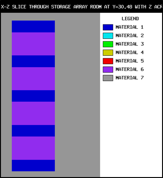
Fig. 8.1.86 X-Z plot of storage array.

The plot data and UNIT map for an X-Y slice through the shelf are given in Example 8.1.33 and Fig. 8.1.87. This UNIT map was created with X across the plot and Y down the plot. This shows five rows of shelves in the X direction.

Example 8.1.33 Plot data for X-Y slice of storage array.

x-y slice through storage array room at z=0.3175 with x across and y down
unit map

    unit  1 2 3 4 5 6 7
  symbol  1 2 3 4 5 6 7
        upper  left          lower right
        coordinates          coordinates
 x     -3.0480e+01           6.2484e+02
 y      1.3411e+03          -3.0480e+01
 z      3.1750e-01           3.1750e-01
           u axis      v axis
           (down)      (across)
 x         0.00000      1.00000
 y        -1.00000      0.00000
 z         0.00000      0.00000
 nu=  669   nv=  320     delu= 2.0479e+00     delv= 2.0479e+00     lpi=  10.000

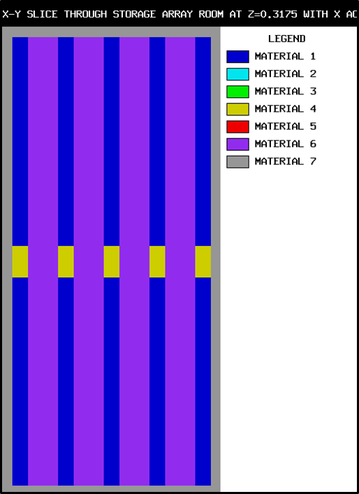
Fig. 8.1.87 X-Y plot of storage array.

8.1.4.11. KENO Multiple Mesh and Mesh-based Quantity Specifications

KENO constructs a grid object and stores several mesh definitions in this object. The following mesh definitions are supported by KENO:

1. Default mesh grid (grid ID =10001):

KENO generates a 5 \(\times\) 5 \(\times\) 5 Cartesian mesh grid which overlays the entire geometry. This mesh is used only for fission source convergence diagnostics if the user does not specify any spatial mesh for this quantity.

Note

Currently, users cannot enter grid IDs greater than 9999.

2. A cubic mesh grid (grid ID = 20001):

KENO generates a cubic mesh with the mesh size specified by MSH parameter, which is introduced in Table 8.1.1. This mesh definition can be used by all mesh-based quantities except the Shannon Entropy tallies used for fission source convergence diagnostics.

3. Mesh with grid geometry data input (grid ID = NUMBER):

The user can specify either a mesh with a single grid data input block or multiple meshes by repeating the grid data input block with different mesh definitions. Note that the entire block, including READ GRID and END GRID, must be repeated each time; this behavior is different from all other blocks of KENO input.

After processing all grid data and constructing all grid meshes, KENO prints the specification of each mesh grid in the Grid Definitions output edit; see Sect. 8.1.5.19 for details.

Before starting the transport process, KENO tries to match the IDs specified in the parameter block with the keywords SCD, MFX, CDS, CGD, FIS, and GFX (See Sect. 8.1.3.3) to the grid ID in each grid definition. Each mesh-based quantity requested by the user is associated with a grid if the requested grid ID exists.

Note

Parameters CDS, CGD, FIS, GFX, and MFX with YES entry always require a mesh defined by either parameter MSH or grid data input.

Parameters CDS, CGD, FIS, GFX, and MFX with YES entry always use the mesh defined by the first grid data input if there are multiple meshes defined by both MSH and grid data input block(s).

The following examples demonstrate the mesh features in KENO:

Example: Source Convergence Diagnostics with Default Mesh

KENO always generates a default mesh for source convergence diagnostics if the user does not specify any mesh for this quantity. The following example (only KENO-VI version is shown) with some updates in parameter data and grid data input blocks will be used in all examples in this section to summarize several mesh definition scenarios with several mesh-based quantity requests.

In this sample problem, a bounding box is defined to enclose the entire geometry with xmin=-13.74, xmax=13.74, ymin=-13.74, ymax=13.74, zmin=-13.01, and zmax=13.01. KENO uses this bounding box and creates a 5 \(\times\) 5 \(\times\) 5 grid for source convergence diagnostics.

KENO-VI:

=kenovi
mesh test - scd with default mesh (5x5x5), scd=yes (default)
READ PARAMETER
   CEP=ce_v7.1_endf NPG=10000
END PARAMETER

read mixt
   mix=1
      92234  4.82716E-04 92235  4.47972E-02
              92236  9.57234E-05 92238  2.65768E-03
end mixt

read geometry
   unit 1
      com='single 2c8 unit centered'
      cylinder 10  5.748 5.3825 -5.3825
      cuboid   20  4p6.87 2p6.505
      media  1 1 10      vol=8938.968624
      media  0 1 20 -10  vol=10710.044784
      boundary 20
   global unit 2
      cuboid 10  4p13.74 2p13.01
      com='2x2x2  2c8 array'
      array 1 +10 place 1 1 1 2r-6.87 -6.505
      boundary  10
end geometry

read array
   ara=1 nux=2 nuy=2 nuz=2  fill f1  end fill
end array
end data
end

In the output, KENO notifies users about the default mesh usage for source convergence diagnostics with the message k6-316. The default grid definition with some details is shown in Example 8.1.34.

Fig. 8.1.88 shows the Fulcrum visualized Shannon Entropy by generations plot for this sample problem.

Example 8.1.34 Grid Definitions output edit

  ***** warning ***** keno message number k6-316 follows:
  No mesh provided for Source Convergence Diagnostics (SCD). Continue with default mesh.

  ...

            ********************************************************************************************************************
      ***                                                                                                              ***
      ***                                         grid definitions                                                     ***
      ***                                                                                                              ***
      ***     Only a single grid geometry is either specified or internally setup for this problem                     ***
      ***                                                                                                              ***
      ********************************************************************************************************************

                                **** Grid geometries utilized in this problem ****

  Grid Geometry: 10001
    title: Default 5 x 5 x 5 Cartesian mesh which overlays the entire geometry
    Plane Summary
      x:    5 cells from -1.37400E+01 to  1.37400E+01
      y:    5 cells from -1.37400E+01 to  1.37400E+01
      z:    5 cells from -1.30100E+01 to  1.30100E+01
    Total number of cells: 125

                        x-planes               y-planes               z-planes
    -----  ---------------------  ---------------------  ---------------------
        1  -1.37400137400000E+01  -1.37400137400000E+01  -1.30100130100000E+01
        2  -8.24400824399998E+00  -8.24400824399998E+00  -7.80600780599998E+00
        3  -2.74800274799999E+00  -2.74800274799999E+00  -2.60200260199999E+00
        4   2.74800274799999E+00   2.74800274799999E+00   2.60200260199999E+00
        5   8.24400824399998E+00   8.24400824399998E+00   7.80600780599998E+00
        6   1.37400137400000E+01   1.37400137400000E+01   1.30100130100000E+01
    -----  ---------------------  ---------------------  ---------------------

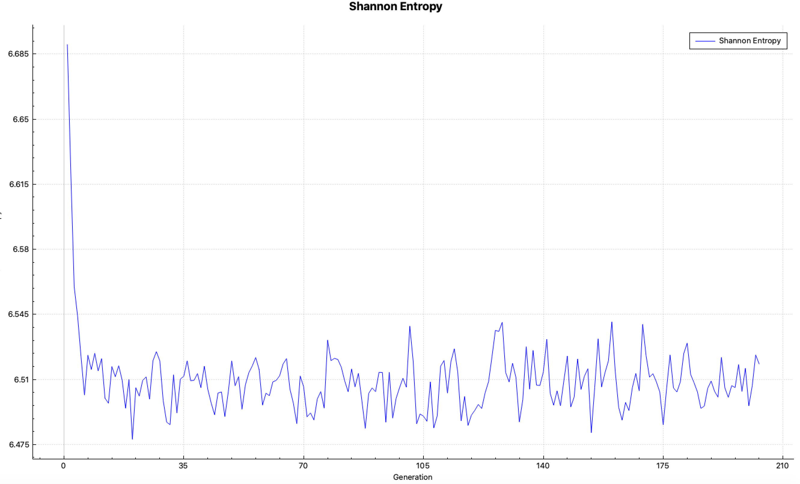
Fig. 8.1.88 Shannon entropy tallied on default mesh.

Example: Source Convergence Diagnostics with User-defined Mesh.

The user can request the accumulation of the fission source on a different grid rather than the default grid for source convergence diagnostics. In this example, the sample problem specified in previous example is modified for this purpose. A new 6 \(\times\) 6 \(\times\) 6 grid is defined over the entire geometry in a grid geometry data input with grid ID 12, and source convergence diagnostics are requested by setting SCD parameter to 12 in the parameter block that matches the NUMBER specification in the grid geometry data input.

=kenovi
mesh test - scd with user-defined grid

READ PARAMETERS
   CEP=ce_v7.1_endf NPG=10000 SCD=12
END PARAMETERS

...

READ GRID
   12
   TITLE "test scd with this mesh"
   NUMXCELLS=6 NUMYCELLS=6 NUMZCELLS=6
   XMIN=-13.74 XMAX=13.74
   YMIN=-13.74 YMAX=13.74
   ZMIN=-13.01 ZMAX=13.01
END GRID
...

Note

Starting from this example, only a summary of Grid Definiton output edit will be presented for the remaining examples.

A User-defined grid is printed in Grid Definitons output edit, and Example 8.1.35 presents only a summary of this output section. Fig. 8.1.89 shows the variation of Shannon Entropy (tallied on user-defined mesh) over generations for the same problem given in the previous example.

Example 8.1.35 Grid Definitions output edit

  ...

      Grid Geometry: 12
    title: test scd with this mesh
    Plane Summary
      x:    6 cells from -1.37400E+01 to  1.37400E+01
      y:    6 cells from -1.37400E+01 to  1.37400E+01
      z:    6 cells from -1.30100E+01 to  1.30100E+01
    Total number of cells: 216

      ...

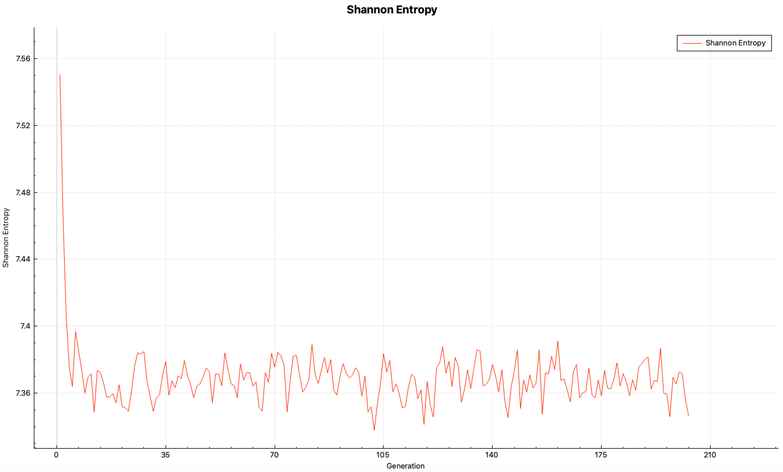
Fig. 8.1.89 Shannon entropy tallied on user-defined mesh.

Example: Source Convergence Diagnostics with Non-Existing Mesh.

This example demonstrates the code behavior if there is a mismatch between the NUMBER entry in grid geometry data input and the SCD parameter in the parameter data. The sample input in the first example was modified as (a) a single mesh is defined with grid ID = 12, and (b) source convergence diagnostics is intended to use a grid with grid ID = 99, which does not exist.

=kenovi
mesh test - scd with non-existing grid id

READ PARAMETERS
   CEP=ce_v7.1_endf NPG=10000 SCD=99
END PARAMETERS

...

READ GRID
   12
   TITLE "test scd with this mesh"
   NUMXCELLS=6 NUMYCELLS=6 NUMZCELLS=6
   XMIN=-13.74 XMAX=13.74
   YMIN=-13.74 YMAX=13.74
   ZMIN=-13.01 ZMAX=13.01
END GRID
...

In this example, calculation is stopped with an error message since the requested grid definition for source convergence diagnostics does not exist in the input.

...

***** error ***** keno message number k6-315 follows:
Mesh < 99 > specified for Shannon entropy tally and source convergence diagnostics(SCD) is not found in  input.

...

***** error ***** keno message number k6-100 follows:
this problem will not be run because errors were encountered in the input data.
...

Example: Fission Rate Mesh Tally with a Cubic Mesh Definition with MSH Parameter.

In this example, the sample problem described in the first example was modified as (a) a cubic mesh defined with the MSH parameter, and (b) fission rate mesh tally is requested on this cubic mesh. In this case, a default mesh with grid ID=10001 is constructed and used only for source convergence diagnostics. The cubic mesh with grid ID=20001 is also constructed with the length of one side as equals to 2.748 cm and is used for the fission rate mesh tally.

=kenovi
mesh test - fis with uniform mesh defined by MSH

READ PARAMETERS
   CEP=ce_v7.1_endf NPG=10000 FIS=yes MSH=2.748
END PARAMETERS

...

The output prints the details of mesh grid entries in Grid Definitions edit, as shown in Example 8.1.36. For this sample problem, the cubic mesh grid is constructed in a box that is larger than the bounding box around the global unit (+x=13.74, -x=-13.74, +y=13.74, -y=-13.74, +z=13.01 and -z=-13.01). The extents of the global boundary in each dimension are not equal; therefore, KENO tries to adjust the box size to place the cubic meshes properly inside this box. A grid mesh perfectly overlapping the problem geometry can be defined only by the grid data input rather than using the MSH parameter.

Example 8.1.36 Grid Definitions output edit

                                **** Grid geometries utilized in this problem ****

Grid Geometry: 20001
      title: Cubic mesh grid automatically generated with mesh_size =   2.74799991
      Plane Summary
        x:   12 cells from -1.64880E+01 to  1.64880E+01
        y:   12 cells from -1.64880E+01 to  1.64880E+01
        z:   12 cells from -1.64880E+01 to  1.64880E+01
      Total number of cells: 1728

                          x-planes               y-planes               z-planes
      -----  ---------------------  ---------------------  ---------------------
          1  -1.64879994392395E+01  -1.64879994392395E+01  -1.64879994392395E+01
          2  -1.37399995326996E+01  -1.37399995326996E+01  -1.37399995326996E+01

...

Grid Geometry: 10001
    title: Default 5 x 5 x 5 Cartesian mesh which overlays the entire geometry
    Plane Summary
      x:    5 cells from -1.37400E+01 to  1.37400E+01
      y:    5 cells from -1.37400E+01 to  1.37400E+01
      z:    5 cells from -1.30100E+01 to  1.30100E+01
    Total number of cells: 125

...

Specifications of fission rate mesh tally in Mesh Tallies output edit are listed in Example 8.1.37. Fission rate mesh tally is saved in a 3dmap file named example4.fission_density.3dmap, and results from this file overlayed on the geometry are shown in Fig. 8.1.90.

Example 8.1.37 Mesh tallies output edit

                                                   **** mesh tallies ****

  1 mesh tallies computed for this problem


   mesh tally (requested with parameter fis)
       response         : fission_density
       grid id          : 20001
       energy id        : Default
       memory allocated : 6.645 MB
       output           : example4.fission_density.3dmap

       energy boundaries:
            group   energy (eV)
           ------  ------------
                1   2.00000E+07
                2   1.73300E+07
                3   1.56800E+07
                .              .
              250   7.50000E-04
              251   5.00000E-04
              252   1.00000E-04
                    1.00000E-05
           ------  ------------

       grid summary:
             x:   12 cells from -1.64880E+01 to  1.64880E+01
             y:   12 cells from -1.64880E+01 to  1.64880E+01
             z:   12 cells from -1.64880E+01 to  1.64880E+01
           Total number of cells: 1728

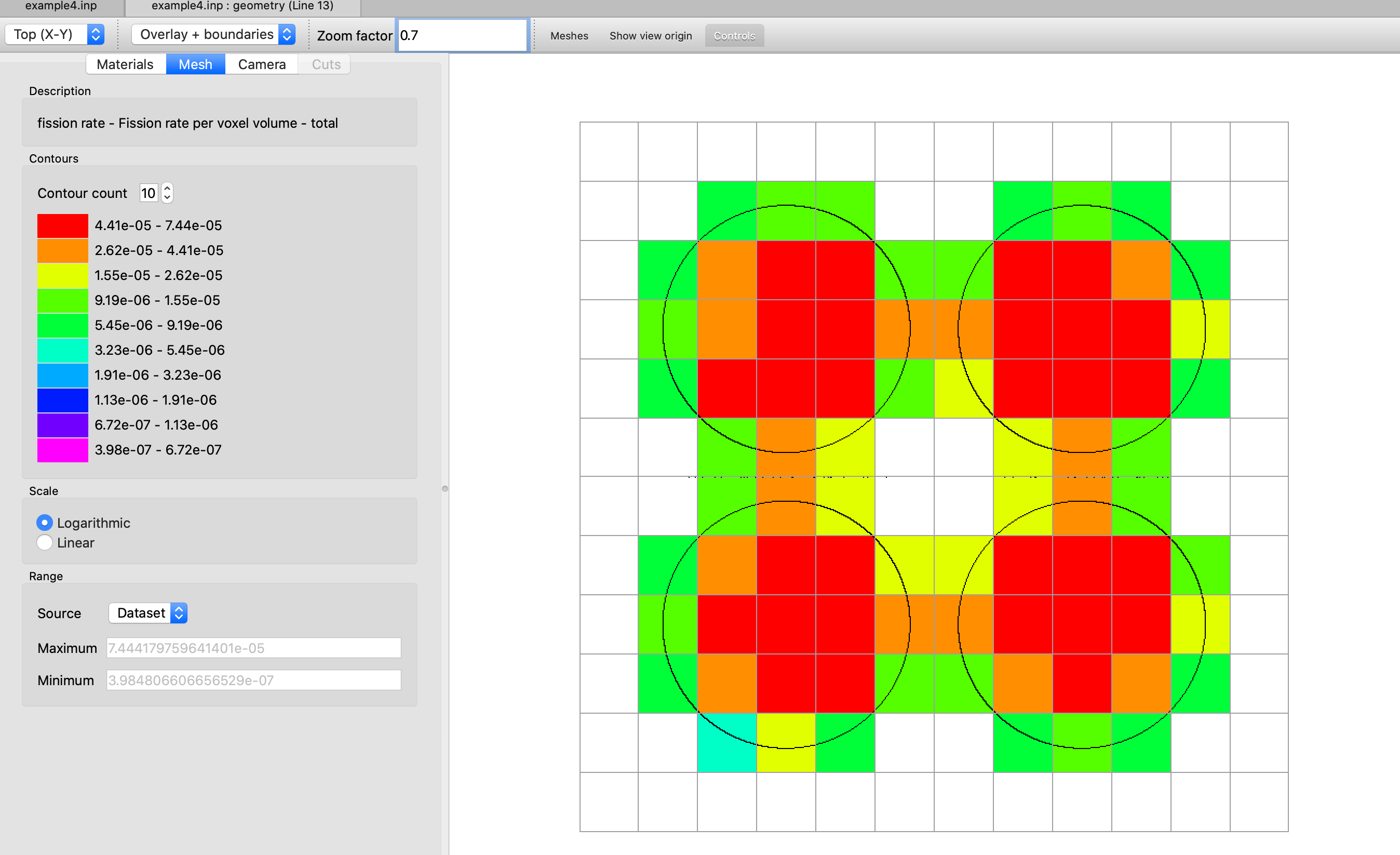
Fig. 8.1.90 Fission rate mesh tally computed on a uniform mesh defined by MSH=2.748 (X-Y view at z=5.0).

Example: Fission Rate Mesh Tally with a NUMBER.

In this example, problem given in the first example was modified to request a fission rate mesh tally calculation over a mesh defined in the grid geometry data input. A default mesh with grid ID=10001 is constructed and used for the source convergence diagnostics. The user defined mesh (grid ID=17) is used for the fission rate mesh tally.

=kenovi
mesh test - fis with a mesh defined by grid data block

READ PARAMETERS
   CEP=ce_v7.1_endf NPG=10000 FIS=17
END PARAMETERS
...

READ GRID
   17
   TITLE "test fis with this mesh"
   NUMXCELLS=20 NUMYCELLS=20 NUMZCELLS=6
   XMIN=-13.74 XMAX=13.74
   YMIN=-13.74 YMAX=13.74
   ZMIN=-13.01 ZMAX=13.01
END GRID
...

A summary of the mesh grids utilized in this sample problem is printed in Grid Definitions, as shown in Example 8.1.38.

Example 8.1.38 Grid Definitions output edit

                                **** Grid geometries utilized in this problem ****

Grid Geometry: 17
    title: test fis with this mesh
    Plane Summary
      x:   20 cells from -1.37400E+01 to  1.37400E+01
      y:   20 cells from -1.37400E+01 to  1.37400E+01
      z:    6 cells from -1.30100E+01 to  1.30100E+01
    Total number of cells: 2400

...

Grid Geometry: 10001
    title: Default 5 x 5 x 5 Cartesian mesh which overlays the entire geometry
    Plane Summary
      x:    5 cells from -1.37400E+01 to  1.37400E+01
      y:    5 cells from -1.37400E+01 to  1.37400E+01
      z:    5 cells from -1.30100E+01 to  1.30100E+01
    Total number of cells: 125

Example 8.1.39 is a snapshot of the Mesh Tallies output edit, which summarizes the specification of this mesh quantity. The fission rate mesh tally is saved in a 3dmap file named example5.fission_density.3dmap. Tally results from this file overlayed over the geometry are shown in Fig. 8.1.91.

Example 8.1.39 Mesh tallies output edit

                                                   **** mesh tallies ****

  1 mesh tallies computed for this problem


   mesh tally (requested with parameter fis)
       response         : fission_density
       grid id          : 17
       energy id        : Default
       memory allocated : 9.229 MB
       output           : example5.fission_density.3dmap

       energy boundaries:
            group   energy (eV)
           ------  ------------
                1   2.00000E+07
                2   1.73300E+07
                3   1.56800E+07
                .              .
              250   7.50000E-04
              251   5.00000E-04
              252   1.00000E-04
                    1.00000E-05
           ------  ------------

       grid summary:
             x:   20 cells from -1.37400E+01 to  1.37400E+01
             y:   20 cells from -1.37400E+01 to  1.37400E+01
             z:    6 cells from -1.30100E+01 to  1.30100E+01
           Total number of cells: 2400

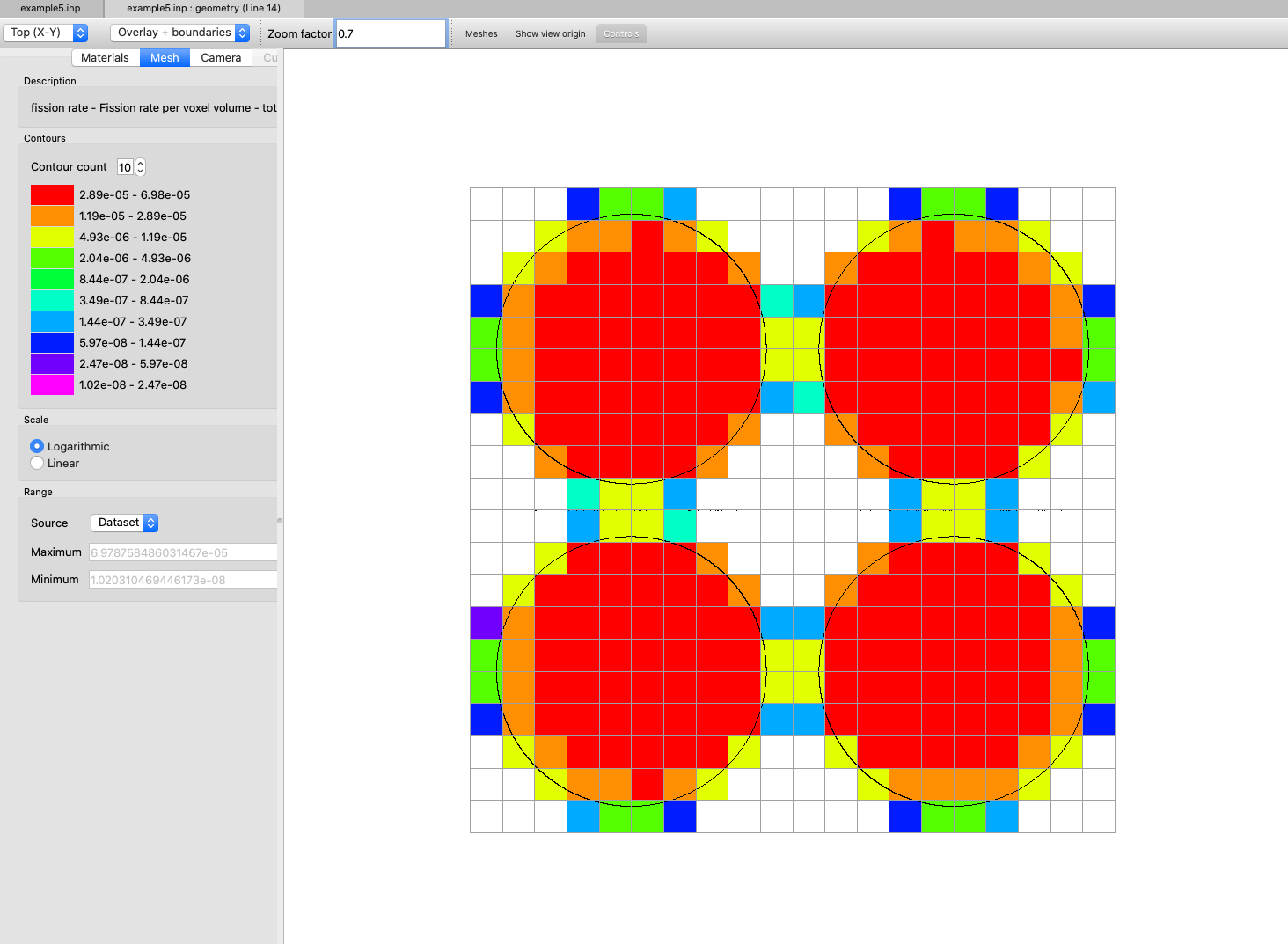
Fig. 8.1.91 Fission rate mesh tally computed on a mesh defined by grid geometry data input (X-Y view at z=5.0).

Example: Fission Rate Mesh Tally with Multiple Mesh Definitions.

In this example, the sample input from the previous example is used with the old-style definition so that fission rate mesh tally is requested by setting the FIS parameter to YES.

Additional mesh grids were added to the sample input to demonstrate how KENO assigns a mesh grid to a mesh-based quantity when the value of mesh quantity has been entered as YES and multiple mesh grids have already been defined: (a) two mesh grids with grid IDs 118 and 113 are defined in grid geometry data inputs, and (b) another mesh grid is also defined with the MSH parameter.

KENO uses the default mesh grid (grid ID=10001) for the source convergence diagnostics, using the mesh with grid ID= 118 from the grid data container for the fission rate mesh tally.

=kenovi
mesh test - fis=yes with multiple mesh defined by grid data block

READ PARAMETERS
   CEP=ce_v7.1_endf NPG=10000 MSH=2.5 FIS=yes
END PARAMETERS
...

READ GRID
   118
   TITLE "test fis with this mesh partially covering the geometry"
   NUMXCELLS=20 NUMYCELLS=20 NUMZCELLS=18
   XMIN=-1.74 XMAX=13.74
   YMIN=-1.74 YMAX=13.74
   ZMIN=-1.01 ZMAX=13.01
END GRID

READ GRID
   113
   TITLE "mesh will not be used"
   NUMXCELLS=3 NUMYCELLS=3 NUMZCELLS=3
       XMIN=-1.74 XMAX=13.74
       YMIN=-1.74 YMAX=13.74
       ZMIN=-1.01 ZMAX=13.01
END GRID

READ GRID
   17
   TITLE "test fis with this mesh"
   NUMXCELLS=20 NUMYCELLS=20 NUMZCELLS=6
   XMIN=-13.74 XMAX=13.74
   YMIN=-13.74 YMAX=13.74
   ZMIN=-13.01 ZMAX=13.01
END GRID


...

A summary of Grid Definitions output edit is given in Example 8.1.40. Note that KENO does not print anything for the cubic mesh (requested by setting MSH=2.5, grid ID= 20001) because this mesh was not constructed. KENO ignores the mesh definition request done with the MSH parameter if any mesh grid is defined by grid data input.

Example 8.1.40 Grid Definitions output edit

                                **** Grid geometries utilized in this problem ****

 Grid Geometry: 118
    title: test fis with this mesh partially covering the geometry
    Plane Summary
      x:   20 cells from -1.74001E+00 to  1.37400E+01
      y:   20 cells from -1.74001E+00 to  1.37400E+01
      z:   18 cells from -1.01001E+00 to  1.30100E+01
    Total number of cells: 7200

...

 Grid Geometry: 113
     title: mesh will not be used
     Plane Summary
       x:    3 cells from -1.74001E+00 to  1.37400E+01
       y:    3 cells from -1.74001E+00 to  1.37400E+01
       z:    3 cells from -1.01001E+00 to  1.30100E+01
     Total number of cells: 27

...

Grid Geometry: 17
    title: test fis with this mesh
    Plane Summary
      x:   20 cells from -1.37400E+01 to  1.37400E+01
      y:   20 cells from -1.37400E+01 to  1.37400E+01
      z:    6 cells from -1.30100E+01 to  1.30100E+01
    Total number of cells: 2400

...

 Grid Geometry: 10001
     title: Default 5 x 5 x 5 Cartesian mesh which overlays the entire geometry
     Plane Summary
       x:    5 cells from -1.37400E+01 to  1.37400E+01
       y:    5 cells from -1.37400E+01 to  1.37400E+01
       z:    5 cells from -1.30100E+01 to  1.30100E+01
     Total number of cells: 125

...

KENO assigns the first grid entry from the grid data container to any mesh quantity whose value is entered as YES in the parameter data input. Each grid defined in the grid data blocks is stored in the grid data container unit in the order in which it is processed.

In this example, the grid entry 118, which is processed and stored first, is assigned to the fission rate mesh tally calculation. Mesh Tallies output edit shown in Example 8.1.41 reflects this grid assignment to the fission ate mesh tally.

Example 8.1.41 Mesh tallies output edit

                                            **** mesh tallies ****

  1 mesh tallies computed for this problem


   mesh tally (requested with parameter fis)
       response         : fission_density
       grid id          : 118
       energy id        : Default
       memory allocated : 27.686 MB
       output           : example6.fission_density.3dmap

       energy boundaries:
            group   energy (eV)
           ------  ------------
                1   2.00000E+07
                2   1.73300E+07
                3   1.56800E+07
                .              .
              250   7.50000E-04
              251   5.00000E-04
              252   1.00000E-04
                    1.00000E-05
           ------  ------------

       grid summary:
             x:   20 cells from -1.74001E+00 to  1.37400E+01
             y:   20 cells from -1.74001E+00 to  1.37400E+01
             z:   18 cells from -1.01001E+00 to  1.30100E+01
           Total number of cells: 7200

...

Fig. 8.1.92 illustrates the fission rate mesh tally overlayed on the geometry. Note that the mesh used in the fission rate mesh tally calculation does not cover the entire geometry, and this is not a requirement for this tally.

Note

The fission rate mesh tally capability as well as fission source and grid flux tallies (averaged over mesh volumes) do not require that the mesh grid used in the calculation cover the entire geometry.

However, the mesh flux capability (calculated over the volume of materials in each mesh voxel) activated by the MFX parameter always requires that the mesh grid used in its calculations cover the entire geometry.

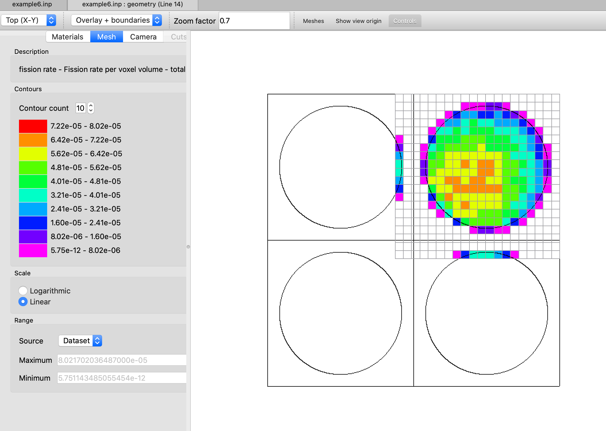
Fig. 8.1.92 Fission rate mesh tally computed over a mesh grid defined by grid geometry data input. Defined mesh grid with ID= 118 partially covers the geometry (X-Y view at z=6.8).

Example: Mesh Flux Tally with Multiple Mesh Definitions.

In this example, the sample problem described in previous example is modified to request a mesh flux calculation (MFX) on a mesh grid which partly covers the problem geometry. The mesh volume calculation required by the mesh flux calculation is already requested by adding a volume block to the input.

Note

Calculation of mesh fluxes in all regions enclosed by a mesh voxel requires the volume of each region in this mesh voxel. KENO V.a automatically activates stochastic volume calculation with RANDOM volume estimate for such a case. The user can override the parameters in the volume data input block. However, users cannot change the volume calculation method from RANDOM volume estimate to TRACE volume estimate.

In the KENO-VI case, it is the user’s responsibility to add a volume data input block to activate the stochastic mesh volume calculation. Like KENO V.a, KENO-VI only allows RANDOM volume estimate for mesh volume calculation. See Sect. 8.1.3.13 and Sect. 8.1.5.17 for more details.

After these updates, KENO with this sample problem uses the default mesh (grid ID=10001) for the source convergence diagnostics, and the user-defined mesh with grid ID=118 for accumulating the mesh fluxes. Unlike the fission rate mesh tally case discussed in the previous example, execution is terminated for this scenario since the mesh flux capability requested with MFX parameter requires a mesh grid covering the entire geometry.

 =kenovi
 mesh test - mfx=yes with a grid mesh covering the part of the geometry

 READ PARAMETERS
    CEP=ce_v7.1_endf NPG=10000 MFX=yes
 END PARAMETERS

...

 READ GRID
    118
    TITLE "test fis with this mesh partially covering the geometry"
    NUMXCELLS=20 NUMYCELLS=20 NUMZCELLS=18
    XMIN=-1.74 XMAX=13.74
    YMIN=-1.74 YMAX=13.74
    ZMIN=-1.01 ZMAX=13.01
 END GRID

 READ GRID
    113
    TITLE "mesh will not be used"
    NUMXCELLS=3 NUMYCELLS=3 NUMZCELLS=3
        XMIN=-1.74 XMAX=13.74
        YMIN=-1.74 YMAX=13.74
        ZMIN=-1.01 ZMAX=13.01
 END GRID

 READ GRID
    17
    TITLE "test fis with this mesh"
    NUMXCELLS=20 NUMYCELLS=20 NUMZCELLS=6
    XMIN=-13.74 XMAX=13.74
    YMIN=-13.74 YMAX=13.74
    ZMIN=-13.01 ZMAX=13.01
 END GRID

 ...

 READ VOLUME
   TYPE=RANDOM BATCHES=100 POINTS=1000
   XP=+13.01  XM=-13.01
   YP=+13.74  YM=-13.74
   ZP=+13.74  ZM=-13.74
 END VOLUME

 ...

The code is stopped with the following error message in the output:

 ...

 ***** warning ***** keno message number k6-316 follows:
 No mesh provided for Source Convergence Diagnostics (SCD). Continue with default mesh.

 1                                          mesh test - fis  with multiple grid data input

                             volumes for those units utilized in this problem

                     Mesh Volume Sampling Parameters
                     -------------------------------

                     The number of points per batch was specified as 1000
                     This gives a sampling density of  5.08931E-02 points per cc per batch.
                     The number of batches is 100

 ***** error ***** keno message number k6-305 follows:
 Mesh fluxes have been specified, but the mesh does not completely cover the geometry.
 The point x=  3.65030E+00 y=  1.90999E+00 z= -1.02504E+01 lies outside the mesh.
 The problem will not be run.  Fix the mesh and resubmit the case.

 ...

  ***** error ***** keno message number k6-100 follows:
  this problem will not be run because errors were encountered in the input data.

 stop code        129
    execution terminated due to errors. completion code 129. cpu time used 3.15388 seconds
 ***Error: Application failed - see messages file for details.

...

Example: Multiple Mesh Quantity with Multiple Mesh Definitions.

This example demonstrates the multiple mesh definition for multiple mesh-based quantities. Our sample problem from a previous example is modified as (a) the source convergence diagnostics and mesh fluxes are requested with (grid ID= 17), (b) grid fluxes are requested with (grid ID= 113), and (c) fission rate mesh tally is requested with YES.

The first grid entry (grid ID=118) in grid geometry data input is assigned to the fission rate mesh tally.

=kenovi
mesh test - test mfx, gfx, and fis together

READ PARAMETERS
   CEP=ce_v7.1_endf NPG=10000 MFX=17 scd=17 gfx=113 fis=yes pms=yes
END PARAMETERS

...

READ GRID
   118
   TITLE "test fis with this mesh partially covering the geometry"
   NUMXCELLS=20 NUMYCELLS=20 NUMZCELLS=18
   XMIN=-1.74 XMAX=13.74
   YMIN=-1.74 YMAX=13.74
   ZMIN=-1.01 ZMAX=13.01
END GRID

READ GRID
   113
   TITLE "mesh will not be used"
   NUMXCELLS=3 NUMYCELLS=3 NUMZCELLS=3
       XMIN=-1.74 XMAX=13.74
       YMIN=-1.74 YMAX=13.74
       ZMIN=-1.01 ZMAX=13.01
END GRID

READ GRID
   17
   TITLE "test fis with this mesh"
   NUMXCELLS=20 NUMYCELLS=20 NUMZCELLS=6
   XMIN=-13.74 XMAX=13.74
   YMIN=-13.74 YMAX=13.74
   ZMIN=-13.01 ZMAX=13.01
END GRID

...

READ VOLUME
  TYPE=RANDOM BATCHES=100 POINTS=1000
  XP=+13.01  XM=-13.01
  YP=+13.74  YM=-13.74
  ZP=+13.74  ZM=-13.74
END VOLUME

...

All three user-defined mesh grids and default mesh grids constructed by KENO are printed in the Grid Definitions output edit as shown in Example 8.1.42. In this output edit, a summary of the volume calculation results performed on the mesh grid 17 is also printed as part of the grid geometry 17 output edit. Further details on the mesh volume calculation can be seen in the volume information edit in the output. All mesh volumes can be printed by setting PMV=YES in the parameter data input (see Table 8.1.1).

Example 8.1.42 Grid Definitions output edit

                                **** Grid geometries utilized in this problem ****

Grid Geometry: 118
    title: test fis with this mesh partially covering the geometry
    Plane Summary
      x:   20 cells from -1.74001E+00 to  1.37400E+01
      y:   20 cells from -1.74001E+00 to  1.37400E+01
      z:   18 cells from -1.01001E+00 to  1.30100E+01
    Total number of cells: 7200
...

Grid Geometry: 113
   title: mesh will not be used
   Plane Summary
     x:    3 cells from -1.74001E+00 to  1.37400E+01
     y:    3 cells from -1.74001E+00 to  1.37400E+01
     z:    3 cells from -1.01001E+00 to  1.30100E+01
   Total number of cells: 27
...

Grid Geometry: 17
   title: test fis with this mesh
   Plane Summary
     x:   20 cells from -1.37400E+01 to  1.37400E+01
     y:   20 cells from -1.37400E+01 to  1.37400E+01
     z:    6 cells from -1.30100E+01 to  1.30100E+01
   Total number of cells: 2400

                       x-planes               y-planes               z-planes
   -----  ---------------------  ---------------------  ---------------------
       1  -1.37400137400000E+01  -1.37400137400000E+01  -1.30100130100000E+01
       2  -1.23660000000000E+01  -1.23660000000000E+01  -8.67333333333333E+00
...
      20   1.23660000000000E+01   1.23660000000000E+01
      21   1.37400137400000E+01   1.37400137400000E+01
   -----  ---------------------  ---------------------  ---------------------
...

   Region volumes in each mesh voxel have been calculated.
     Total number of volume elements   : 7468
     Number of non-zero volume elements: 3734
   Mesh/region pairs indexed together to speed up mesh flux scoring.

KENO prints the summary of the specifications of the mesh quantities computed in Mesh tallies output edit as shown in Example 8.1.43. The code saves the fission rate mesh tally and grid fluxes in two separate 3dmap files named example8.fission_density.3dmap and example8.flux.3dmap, respectively. Mesh fluxes are also saved in an ASCII file since the PMS parameter is set to YES. Fig. 8.1.93 presents the fission rate mesh tally, grid fluxes, and Shannon entropy computed on the meshes defined in grid geometry data input.

Example 8.1.43 Mesh tallies output edit

...
                                                     **** mesh tallies ****

  2 mesh tallies computed for this problem


   mesh tally (requested with parameter gfx)
       response         : flux
       grid id          : 113
       energy id        : Default
       memory allocated : 0.104 MB
       output           : example8.flux.3dmap

       energy boundaries:
            group   energy (eV)
           ------  ------------
                1   2.00000E+07
                2   1.73300E+07
                3   1.56800E+07
                .              .
              250   7.50000E-04
              251   5.00000E-04
              252   1.00000E-04
                    1.00000E-05
           ------  ------------

       grid summary:
             x:    3 cells from -1.74001E+00 to  1.37400E+01
             y:    3 cells from -1.74001E+00 to  1.37400E+01
             z:    3 cells from -1.01001E+00 to  1.30100E+01
           Total number of cells: 27


  mesh tally (requested with parameter fis)
       response         : fission_density
       grid id          : 118
       energy id        : Default
       memory allocated : 27.686 MB
       output           : example8.fission_density.3dmap

       energy boundaries:
            group   energy (eV)
           ------  ------------
                1   2.00000E+07
                2   1.73300E+07
                3   1.56800E+07
                .              .
              250   7.50000E-04
              251   5.00000E-04
              252   1.00000E-04
                    1.00000E-05
           ------  ------------

       grid summary:
             x:   20 cells from -1.74001E+00 to  1.37400E+01
             y:   20 cells from -1.74001E+00 to  1.37400E+01
             z:   18 cells from -1.01001E+00 to  1.30100E+01
           Total number of cells: 7200

...

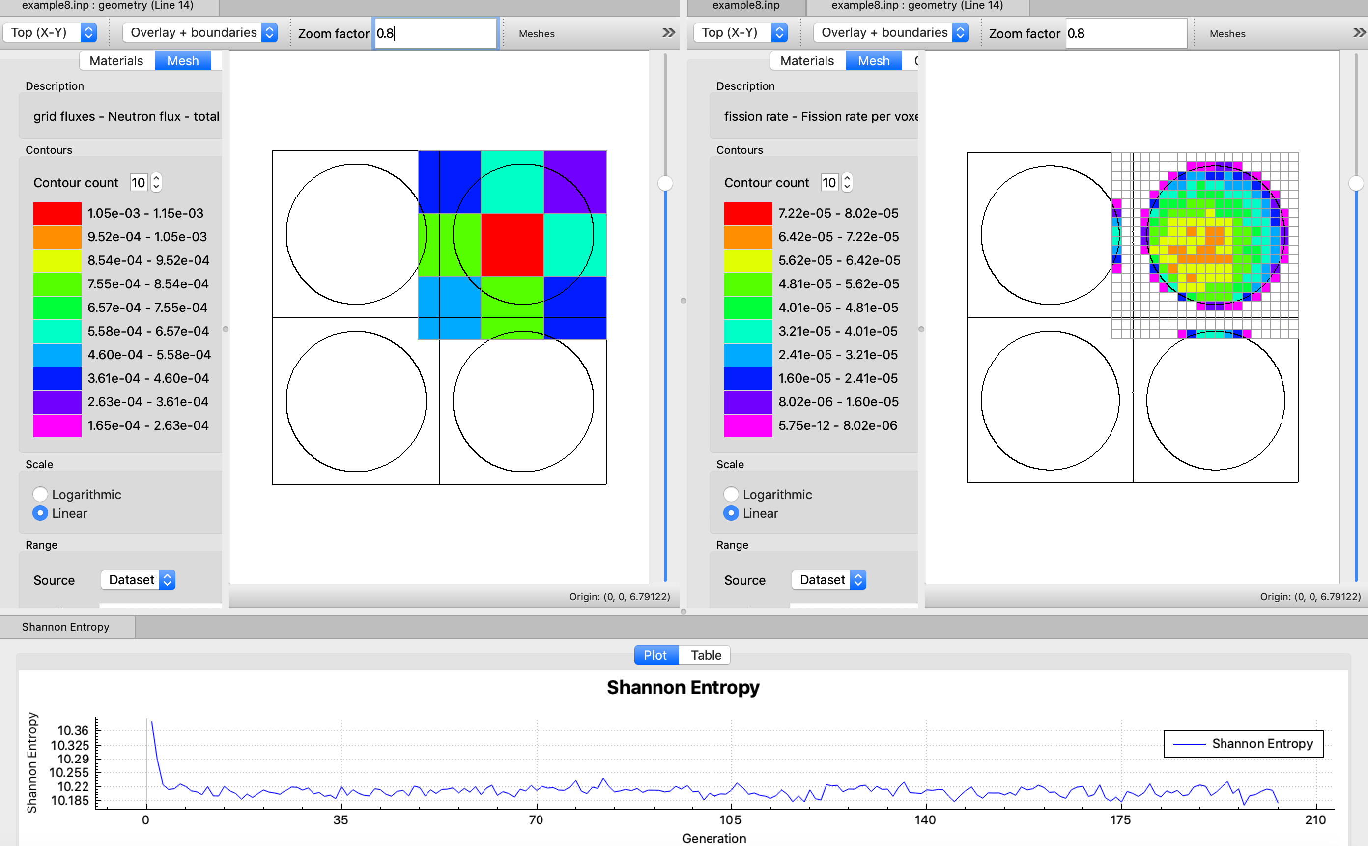
Fig. 8.1.93 Fission rate mesh tally, grid fluxes, and Shannon entropy computed over the different meshes defined by grid geometry data input.

8.1.4.12. Random sequence

The random-number package used by KENO always starts with the same seed and thus always reproduces the same sequence of random numbers. Any random number except the one printed as the starting random number in the parameter table can be used to activate a different random sequence. The user can rerun a problem with a different random sequence by simply entering a hexadecimal random number other than the starting random number in the parameter data. For example, by entering RND=A10C1893E6D5 in the parameter data, the problem will be run with a different random sequence.

8.1.4.13. Matrix k-effective

Matrix k-effective calculations provide an alternative method of calculating the k-effective of the system. Cofactor k-effectives and source vectors are additional information that can be provided when the matrix k-effective is calculated. The necessary source and fission weight data are collected during the neutron tracking procedure. This information is converted to a FISSION PRODUCTION MATRIX, which is the number of next generation neutrons produced at J by a neutron born at I. The principal eigenvalue of the fission probability matrix is the matrix k-effective. KENO offers four alternatives when calculating matrix k-effective as discussed below:

(1) If MKP=YES is specified in the parameter data, the fission production matrix is collected by array position or position index in the GLOBAL ARRAY. The position index is used to reference a given location in a 3-D lattice. For a 2 \(\times\) 2 \(\times\) 2 array, there are nine unique position indices as shown below. Position zero contains everything outside the GLOBAL ARRAY.

Table 8.1.29 Array index guide for a sample 2 \(\times\) 2 \(\times\) 2 array

	POSITION
	X	Y	Z
0	0	0	0
1	1	1	1
2	2	1	1
3	1	2	1
4	2	2	1
5	1	1	2
6	2	1	2
7	1	2	2
8	2	2	2

The fission production matrix is the number of next generation neutrons produced at index J by a neutron born at index I. This matrix is used to calculate the matrix k-effective, cofactor k-effectives and the source vector by position index. Because the size of the fission probability matrix is the square of the array size (for a 4 \(\times\) 4 \(\times\) 4 array there are 4,096 entries), it can use vast amounts of computer memory.

(2) If MKU=YES is specified in the parameter data, the fission production matrix is collected by UNIT. It is the number of next generation neutrons produced in UNIT J by a neutron born in UNIT I. This matrix is used to calculate the matrix k-effective, cofactor k-effectives and source vector by UNIT.

(3) If MKH=YES is specified in the parameter data, the fission production matrix is collected by the HOLE number. Matrix information can be collected at either the highest HOLE nesting level (first level of nesting) or the deepest HOLE nesting level. HHL=YES specifies that the matrix information will be collected at the first nesting level. By default, the matrix information is collected at the deepest nesting level. The fission production matrix is the number of next generation neutrons produced in HOLE J by a neutron born in HOLE I. This matrix is used to calculate the matrix k-effective, cofactor k-effectives and the source vector by HOLE.

(4) If MKA=YES is specified in the parameter data, the fission production matrix is collected by ARRAY number. It can be collected at the highest ARRAY level (first level of nesting) or at the deepest ARRAY level. HAL=YES specifies that the matrix information will be collected at the first nesting level. By default, the matrix information is collected at the deepest nesting level. The fission production matrix is the number of next generation neutrons produced in ARRAY J by a neutron born in ARRAY I. This matrix is used to calculate the matrix k-effective, cofactor k-effectives and the source vector by ARRAY.

The user can simultaneously implement all methods of calculating the matrix k-effective. The results are labeled in the printout. Matrix k-effectives cannot be calculated for a single unit problem. If the user wishes to do so, the geometry description must have a cube or cuboid as its outer region, and the problem description should include READ ARRAY END ARRAY. These two actions convert the single unit problem into a 1 \(\times\) 1 \(\times\) 1 array.

A cofactor k-effective is the eigenvalue of the fission production matrix reduced by the row and column that references the specified UNIT or position index. The difference between the k-effective for the system and the cofactor k-effective for a UNIT or position index is an indication of the in situ k-effective of that UNIT or the contribution that UNIT makes to the k-effective of the system. The cofactor k-effective of a UNIT devoid of fissile material should approximate the k-effective of the system.

8.1.4.14. Deviations

When a deviation is calculated by KENO, it is the standard deviation of the mean. This assumes a large sample having a normal distribution. KENO calculates the real variance using an iterative approach and lag covariance data between generations as follows [Dem99a, UMN97]

1. The sample variance and covariance estimates are calculated.

2. The apparent variance is set equal to the sample variance and the apparent covariance is set equal to the sample covariance.

3. The real covariance is set equal to the apparent covariance and the real variance is calculated.

4. Using the real variance and apparent covariance calculate the real covariance.

5. The real variance is recalculated.

6. Steps 4 and 5 are repeated until the real variance converges within a preset tolerance.

The covariance estimates are only calculated for the previous 20 generations. A maximum of 50 iterations are allowed for the real variance to converge.

8.1.4.15. Generation time and lifetime

The generation time and lifetime calculations use the average velocity. The validity of these calculations is determined by how accurately the average velocity represents the spectrum over the range of the energy group. The lifetime and generation time calculated by KENO are not kinetics parameters. The lifetime is the average life span of a neutron (in seconds) from the time it is born until it is absorbed or leaks from the system. The generation time is the average time (in seconds) between successive neutron generations.

8.1.4.16. Energy of the Average Lethargy of Fission

The energy of the average lethargy of neutrons causing fission (EALF) is a parameter calculated in KENO to characterize the neutron energy spectrum or fastness of a system. The EALF is given in units of eV in the KENO output. An EALF value that is high (> 100 keV) indicates that most fissions in the system are being caused by fast neutrons, and an EALF value that is low (< 1 eV) indicates that most fissions are induced by thermal neutrons.

The EALF is calculated by determining the lethargy, \(u\), a measure of how much neutron energy changes from its initial or birth energy:

(8.1.1)\[u = ln\left( \frac{E_{0}}{E} \right),\]

where \(E\) is the energy of the neutron colliding with a nucleus and \(E_{0}\) is the maximum possible energy of fission neutrons (assumed in KENO to be 10 MeV). The average lethargy of all fission events is calculated by weighting the lethargy for each collision by the probability that the collision will create a fission event, and averaging this quantity. Using a log-scale parameter like lethargy to represent the fastness of systems is more convenient than directly averaging the energy of neutrons causing fission both because of the wide range of neutrons in a problem (potentially more than seven orders of magnitude), and because fast neutrons that are slowing down lose about the same fraction of their energy during each collision.

(8.1.2)\[EALF = E_{o}e^{- u_{\text{avg}}}\]

Equation Eq. (8.1.2) is then applied again to transform the average lethargy of neutrons causing fission into a neutron energy that corresponds to the average lethargy of neutrons causing fission (this is the EALF); this transformation back to units of energy is done because energy has a much more intuitive meaning than units of lethargy.

8.1.5. Description of Output

This section contains a brief description and explanation of the KENO output. Portions of the printout will not be printed for every problem. Some printout is optional, as noted in this section. This section provides representative samples of the output format. The actual data contained in this section are not necessarily consistent with results computed by the current version of KENO.

KENO offers an HTML output format including a series of files that can be viewed in a standard web browser. The HTML formatted output offers interactive output that is easy to read and navigate. Many of the tables of data can be sorted in ascending or descending order by clicking on the heading of the column for which sorting is desired. In this section, the standard text output description is followed by a description of the optional HTML formatted output. The HTML formatted output can be deactivated by entering HTM=NO in the parameter data section.

Warning

The HTML-formatted output is no longer actively developed, and the output files created with it may therefore not include recently added capabilities or changes. For example, the fission rate mesh tally and some CE TSUNAMI edits are not included in the HTML output.

8.1.5.1. Program verification information

Program verification information Fig. 8.1.94 is printed after the header page. It lists the name of the program, the date the load module was created, the library that contains the load module, the computer code name from the configuration control table, and the revision number. The job name, date, and time of execution are also printed. This information may be used for quality assurance purposes.

Fig. 8.1.94 Sample program verification table.

The program verification information is the first page shown in the KENO HTML output, after selecting KENO from the SCALE HTML index page. This page can also be displayed by selecting the Program Verification Information link under the General Information submenu and is shown in Fig. 8.1.94.

8.1.5.2. Tables of parameter data

The first two tables printed by KENO list the numeric parameters and logical parameters used in the problem. The user should always verify that the parameter data block was entered as desired. An example of numeric parameters table is shown in Fig. 8.1.95. An example of the logical parameters table is shown in Fig. 8.1.96.

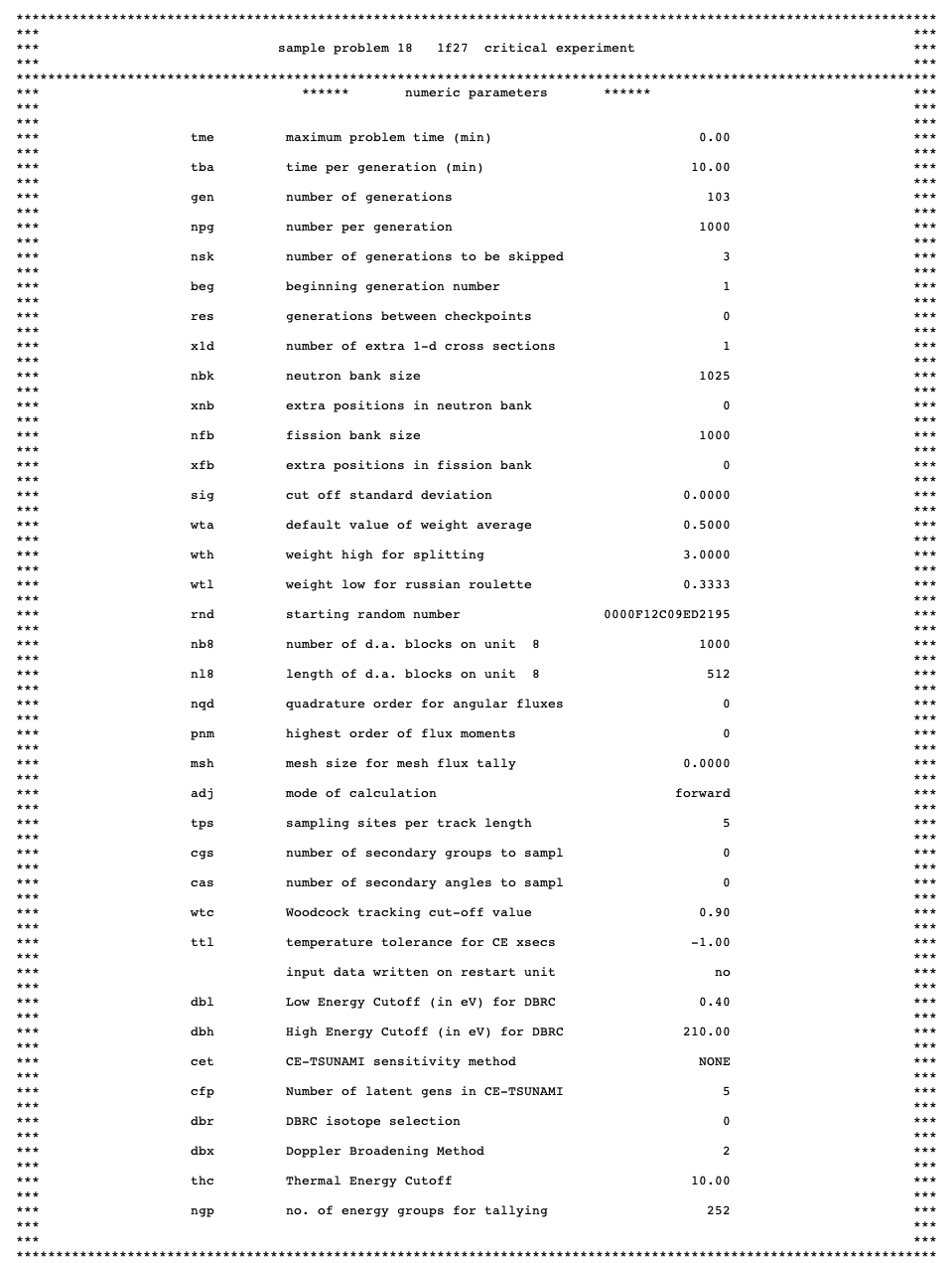
Fig. 8.1.95 Sample table of numeric parameter data.

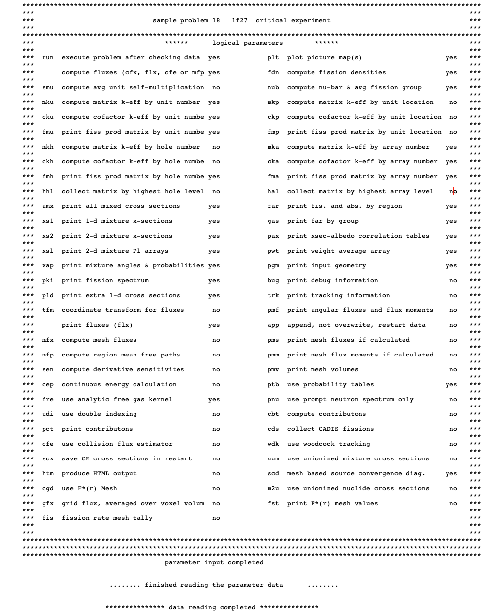
Fig. 8.1.96 Sample table of logical parameter data.

For the logical parameter data table, messages concerning the parameter data may be printed at the bottom of the table. If the problem is being restarted, the title of the parent case is printed at the bottom of the table. If the restart title or messages are not printed, the bottom section of the table is omitted.

8.1.5.3. Unprocessed geometry input data

This printout is optional and is usually used to locate code difficulties, to show all the geometry input data when only part of it is used in the problem, or to show the order in which units were entered. It is considered debug information and is printed only if PGM=YES is specified in the parameter input data. Standard KENO use does not require printing these data because the processed geometry that is used in the problem is always printed. See Sect. 8.1.5.56.9 and Sect. 8.1.5.15 for examples of the standard printed KENO geometry data.

When the unprocessed geometry input is printed, the problem title is located at the top of the page, followed by the heading “GEOMETRY DESCRIPTION INPUT.” The region-dependent geometry information is then printed. If the problem contains a unit orientation array, the problem title is printed again, followed by the unit orientation. This is followed by a statement affirming the completion of the data input.

8.1.5.4. Table of data sets used in the problem

This table is the third table of data printed by KENO. It should be carefully scrutinized to verify the desired data set name is associated with the proper unit number and volume. An example of this table is shown in Fig. 8.1.97.

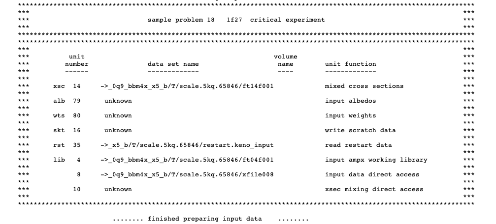
Fig. 8.1.97 Sample table of data sets used in the problem.

This table lists unit numbers specified in the parameter data or that are defaulted in the code, along with the information pertinent to them. This information is given in the following order, left to right: (1) the keyword used in the parameter data to define the unit number, (2) the unit number, (3) the data set name, (4) the name of the volume on which the data set resides, and (5) the type of data contained on the data set. This table can be useful for quality assurance purposes. Information for units for which default values have not been overridden is printed even though they may not be used in the problem. Information for every unit specified in the parameter data is also printed. Units 8 and 10 are the direct-access devices, and their unit numbers are fixed within the code. When this table is printed, Unit 10 has not yet been defined. This causes its data set names to be listed as FT10F001 or as “UNKNOWN” on some systems. If KENO is run as part of a CSAS sequence, this table will include two entries for Unit 35: one for binary input data, and one for read restart data.

8.1.5.5. Table of additional information

The fourth table of data printed by KENO contains additional information determined from the input data. An example of this table is shown in Fig. 8.1.98.

This table should be used to verify the problem input. The NUMBER OF ENERGY GROUPS for a multigroup problem is read either from the Monte Carlo formatted library, identified by the keyword XSC and the unit function name MIXED CROSS SECTIONS from the Table of Data Sets in Sect. 8.1.5.4, or from the restart unit, identified by the keyword RST and the unit function name, READ RESTART DATA. The NO. OF FISSION SPECTRUM SOURCE GROUP is the number of different energy groups for which a fission spectrum is defined. In the present version, this number should always be 1. The NO. OF SCATTERING ANGLES IN XSECS is the number of scattering angles to be used in processing the cross sections. The default value is 3, and it may be overridden by specifying the parameter SCT= in the mixing table input. One scattering angle yields P₁ cross sections, two scattering angles yield P₃ cross sections, three scattering angles yield P₅ cross sections, etc.

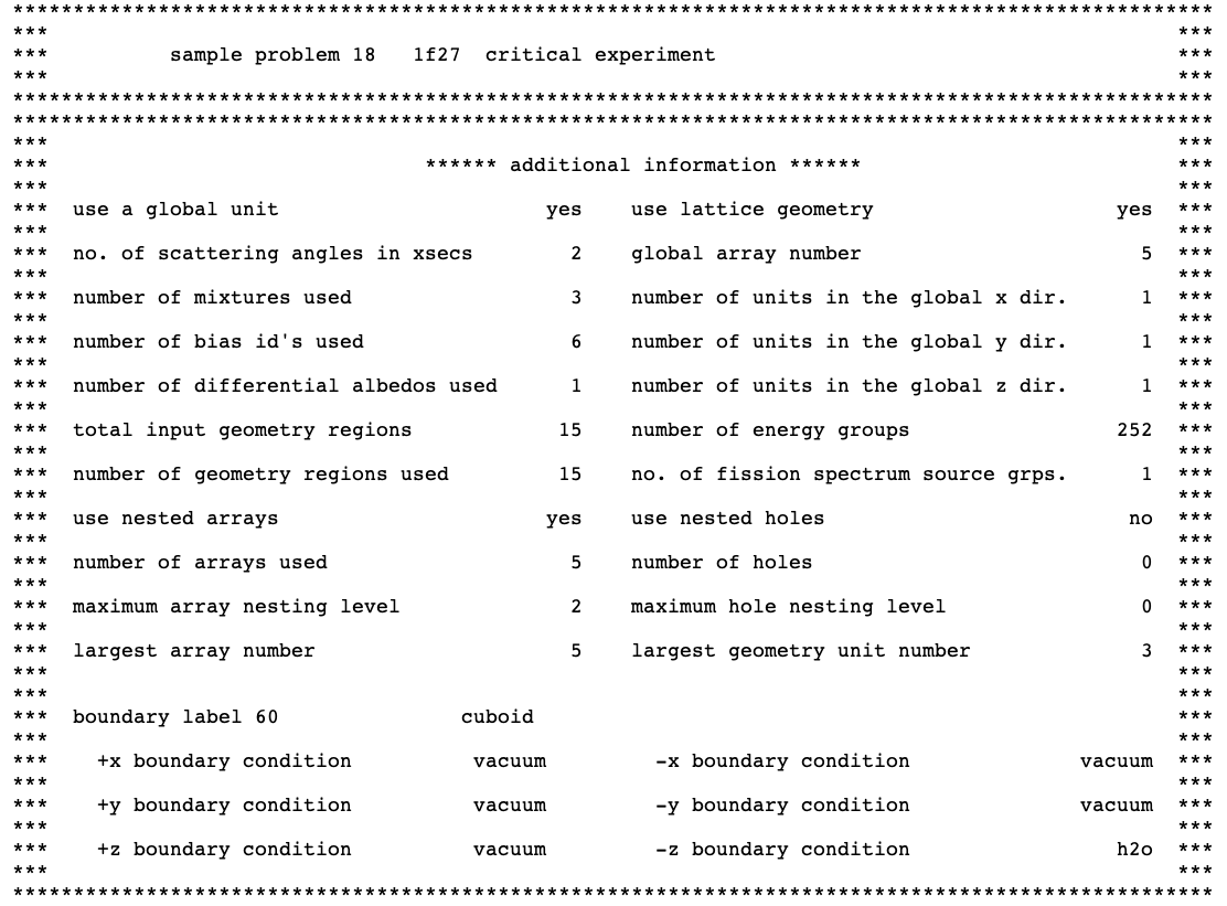
Fig. 8.1.98 Sample table of additional information.

The NUMBER OF MIXTURES USED is the number of different mixtures (media) used in the geometry data used by the problem. This may be less than the total number of different mixtures specified in the geometry data if portions of the geometry data are not used in the problem.

The NUMBER OF BIAS IDS USED is the number of different biasing regions used in the problem. This will always be one unless a biasing data block is entered.

The NUMBER OF DIFFERENTIAL ALBEDOS USED is the number of different differential albedo reflectors used in the problem. This will always be zero unless the boundary condition data specify the use of differential albedo reflection on one or more faces of the system as described in Sect. 8.1.5.8. The BOUNDARY CONDITION data printed in this table should also be checked. The number of different differential albedos specified on the faces should be consistent with the NUMBER OF DIFFERENTIAL ALBEDOS USED. Specular, mirror, vacuum, and periodic are not differential albedos. Several different keywords may be used to specify the same differential albedo.

The TOTAL INPUT GEOMETRY REGIONS is the number of geometry regions specified in the problem input. This excludes UNIT label and comments provided using COM=, but it includes the array boundary description. It excludes the automatic reflector description, but it includes the geometry regions generated by it. The NUMBER OF GEOMETRY REGIONS USED is the number of geometry regions used in the problem. It may be less than or equal to the TOTAL INPUT GEOMETRY REGIONS. The LARGEST GEOMETRY UNIT NUMBER is the largest unit number defined in the geometry data, including unused units and implicitly defined units. Implicitly defined unit numbers are created when a core boundary specification is not immediately preceded by a specification. The unit number is assigned by the code by adding one to the largest unit number encountered in the geometry region data. For example, if two such core boundary specifications are contained in a problem whose largest explicitly defined unit number is 7, then a unit number of 8 is assigned to the first one, and a unit number of 9 is assigned to the second one. A value of 9 would be printed for the LARGEST GEOMETRY UNIT NUMBER. The LARGEST ARRAY NUMBER is the largest array number specified in the array data.

USE LATTICE GEOMETRY is determined by the logical flag that indicates whether or not the problem is a single unit problem. This should be YES for any problem that is not a single unit problem and NO for a single unit problem. By definition, a single unit problem does not use array data in any form. Sect. 8.1.5.14 describes array data. The GLOBAL ARRAY NUMBER is the number of the array designated as the global, overall, or universal array. The global array can be thought of as the array that defines the overall system.

The NUMBER OF UNITS IN THE GLOBAL X/Y/Z DIR. defines the size of the global array in terms of the number of units that are located along the edge of the array boundaries in the X/Y/Z directions. For a single unit, all three of these should be zero. For a simple 1 \(\times\) 1 \(\times\) 1 array consisting of one unit type, all three of these numbers should be 1.

USE NESTED HOLES is set YES if holes are nested deeper than one level.

NUMBER OF HOLES is the number of HOLES that are entered in the geometry region data.

The MAXIMUM HOLE NESTING LEVEL is the deepest level of hole nesting.

USE NESTED ARRAYS is set YES if arrays are nested deeper than one level.

The NUMBER OF ARRAYS USED is the number of array descriptions actually used in the problem description.

MAXIMUM ARRAY NESTING LEVEL is the deepest level of array nesting.

BOUNDARY CONDITIONs are printed near the bottom of the table. They show the type of boundary condition that is applied to each surface of the system. These should all be VACUUM unless albedo boundary conditions are applied to one or more faces of the system. One should refer to the NUMBER OF DIFFERENTIAL ALBEDOS USED, as discussed previously in the description of this table of information.

The outer boundary of the global unit can consist of multiple shapes in KENO-VI geometry. For such a case, BOUNDARY CONDITIONS are printed for all shapes enclosing the global unit as shown in Fig. 8.1.99.

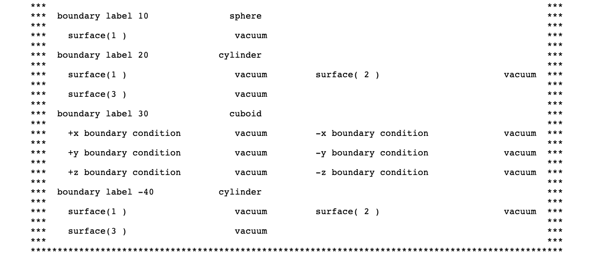
Fig. 8.1.99 Boundary conditions of a KENO-VI model in which combination of multiple shapes encloses the global unit.

Note

Boundary condition edit in Table of additional information does not list the surfaces added to each boundary body by CHORD operations.

8.1.5.6. Cross section data edits for the continuous energy mode

Unlike with the multigroup mode, KENO with continuous-energy mode loads each nuclide data directly from libraries. When loading data, Doppler broadening temperature correction (controlled by DBX parameter, see Sect. 8.1.7.2.10 for further details) is performed by default, on all nuclide cross sections, if the requested temperature is more than 4 K from the library temperature. If the Doppler broadening temperature correction is not enabled, then the nuclides’ data are loaded from libraries with the closest temperature. When running KENO standalone, material temperatures can be entered by the TEMP parameter in the MIXT data block. When running KENO as part of a SCALE sequence, all material temperatures can be entered by each composition data definition in the COMPOSITION data block.

Cross sections data edits in KENO output summarize the data setup in the continuous-energy calculations. Examples of this summary are given in Fig. 8.1.100 and Fig. 8.1.101 for a sample continuous-energy calculation with and without Doppler broadening temperature correction.

This edit starts with printing the thermal energy cutoff utilized in the problem that, followed by a diagnostic edit, notifies that inverse velocity calculations have completed. In the next section, nuclide id, temperature at which data are being processed, and name of temperature-independent and -dependent cross section data files loaded are printed. When Doppler broadening temperature correction has been enabled (DBX= 2), one of the temperature-dependent data files used in this correction is printed as shown in Fig. 8.1.100. This is one of the caveats of this edit since full details of broadening are not listed here. Some messages from the cross section data loader related to broadening can be shown in the message file. After this section, nuclides for which DBRC data loaded are listed if DBRC has been enabled in the calculations. Finally, elapsed time required for data processing (loading + broadening) is reported.

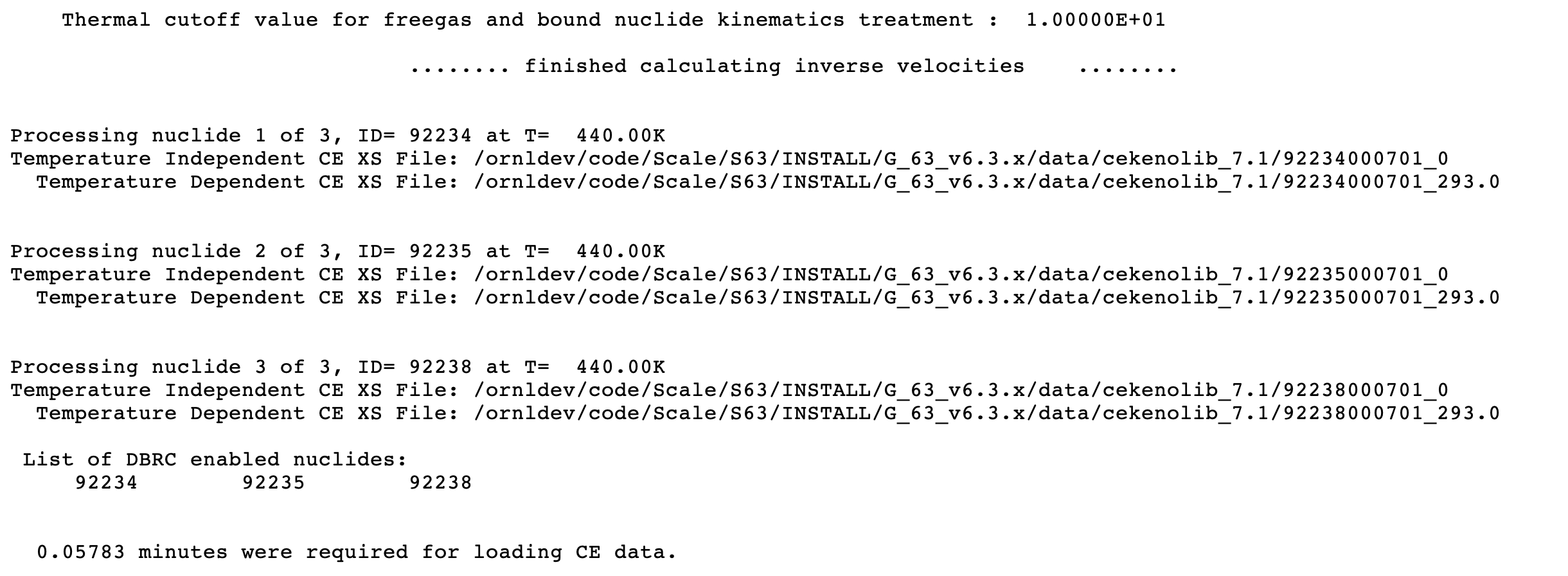
Fig. 8.1.100 Example of cross section data summary for continuous-energy mode (with DBX=2, DBRC=2)

When Doppler broadening temperature correction is turned off (DBX= 0), KENO loads the temperature-dependent data from libraries with the closest temperature and prints their names as shown in Fig. 8.1.101. KENO always notifies the user with a warning message as shown in Fig. 8.1.101 if there is a difference between the temperature at which data would be loaded and the closest temperature for which data has been loaded.

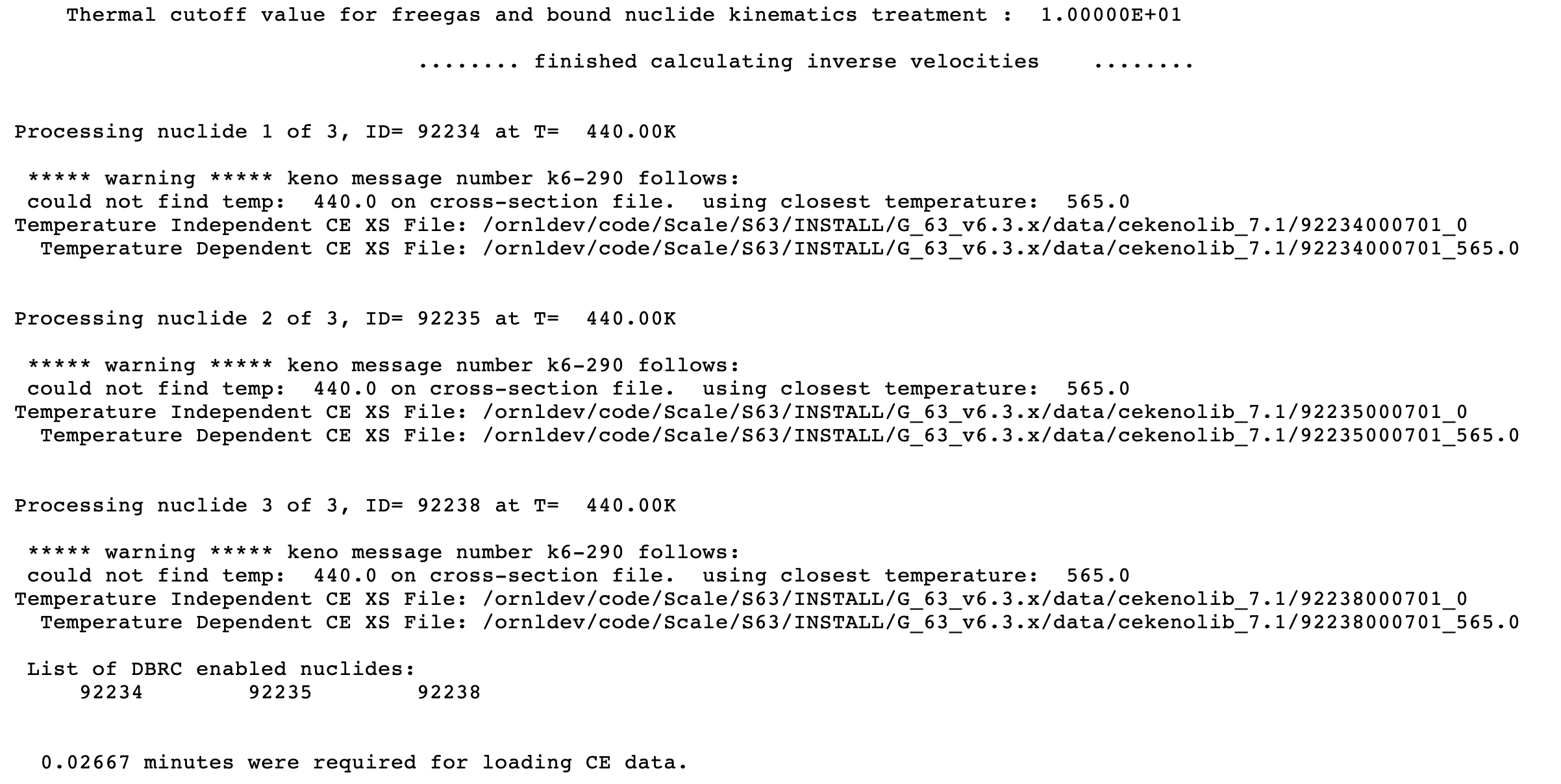
Fig. 8.1.101 Example of cross section data summary for continuous-energy mode (with DBX=0, DBRC=2)

Note

Mixture temperatures printed in the mixing table output edit discussed in the next section are the user-defined temperatures at which cross section data processing has been requested. On the contrary, nuclide temperatures printed in the mixing table output edit show the exact temperatures utilized at which nuclide data are processed for the current calculation.

8.1.5.7. Mixing table data edits

If LIB= is entered in the KENO parameter data and a mixing table data block is provided to KENO, mixing table data will be printed. This output edit is not considered optional because it cannot be suppressed if the necessary data are present. There are some differences between the mixing table data edits for both multigroup and continuous-energy modes.

8.1.5.7.1. Multigroup mode mixing table data edit

Sample mixing table data for multigroup mode are shown in Fig. 8.1.102. In the HTML output, the mixing table data can be accessed with the Mixing Table link in the Input Data section.

The data printed in this table include the problem title, the number of scattering angles, and the cross section message threshold. Data are then printed for each mixture. First the mixture number, density, and temperature are printed, followed by a table of the nuclides which make up the mixture. This table contains the following data: nuclide ID number, nuclide mixture ID number, atom density, weight fraction of nuclide in mixture, ZA number, atomic weight, temperature, and nuclide title. Mixture temperature is the same as the nuclides’ temperatures for the multigroup calculations. After all mixture data have been printed, a table of nuclides and descriptive titles is printed for all nuclides included in the mixtures. If extra 1-D cross sections were specified in the problem (see X1D=, Sect. 8.1.3.3), the extra 1-D cross section IDs will be printed under the heading “1-D CROSS SECTION ARRAY ID NUMBERS.” If \(\bar{\nu}\) is to be calculated (parameter NUB=YES), six MT numbers will be printed. The MT number for the total cross section (\(\Sigma_{\mathrm{T}}\)) is 1; the MT number for the sum of the transfer array normalized by \(\Sigma_{\mathrm{T}}\) is 2002; the MT number for the normalized fission-product cross section \(\left(v \Sigma_{\mathrm{f}} / \Sigma_{\mathrm{t}}\right)\) is 1452; the MT number for the normalized absorption cross section \(\left(\sum_{\mathrm{abs}} / \Sigma_{\mathrm{T}}\right)\) is 27; the MT number for the normalized fission cross section \(\left(\Sigma_{\mathrm{f}} / \Sigma_{\mathrm{T}}\right)\) is 18; and the MT number for the fission spectrum (\(\chi\)) is 1018. \(\chi\) is summed and normalized to 1.0. Other MT numbers in this list have been specified by the user. If the number of blocks on the direct access data set are insufficient to hold the cross section data, a message is printed stating THE NUMBER OF DIRECT ACCESS BLOCKS ON UNIT_____ HAS BEEN INCREASED TO ____. If the problem is to write a restart data set (parameter RES=), a message is printed stating that restart information was written, and the restart I/O unit number is specified. This is followed by a statement of the number of I/Os used in preparing the cross sections. The user should examine the mixing table carefully to verify that the proper nuclides are specified for the proper mixtures and that all the data are correct. The mixing table is printed in subroutine PRTMIX.

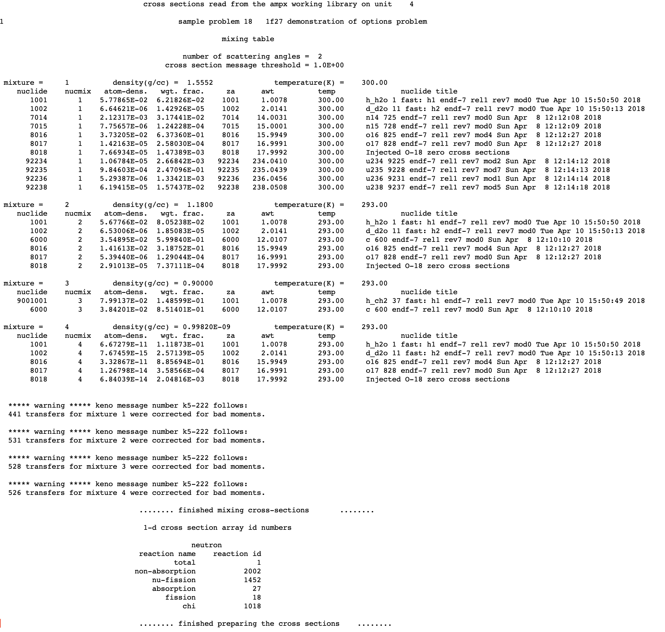
Fig. 8.1.102 Example of mixing table data for multigroup mode.

Note

See Sect. 8.1.4.4.4 for the details for the warning message printed in mixing table edit.

8.1.5.7.2. Continuous-energy mode mixing table data edit

In continuous energy mode, each mixture data is printed immediately after the problem title. For a mixture, first the mixture number, density, and temperature are printed, followed by a table of the nuclides which make up this mixture. Format of the nuclide edits in this table is same as the one used for multigroup mode, it contains the following data: nuclide ID number, nuclide mixture ID number, atom density, weight fraction of nuclide in mixture, ZA number, atomic weight, temperature, and nuclide title.

Sample mixing table data for continuous-energy mode are shown in Fig. 8.1.103. The nuclides’ titles are relatively short compared to those for the multigroup mode since these data are not provided by AMPX, and KENO creates a short title while loading each nuclide data from the continuous-energy libraries.

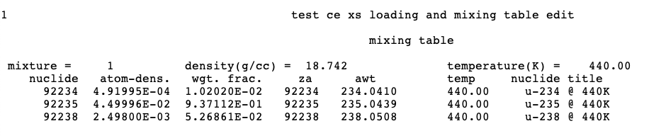
Fig. 8.1.103 Example of mixing table data for continuous energy mode with DBX=2.

Unlike the multigroup calculations, mixture temperature may be different from the nuclides’ temperatures for the continuous-energy calculations if Doppler broadening temperature correction is not enabled (setting DBX= to 0 disables the temperature correction) because the nuclides are loaded from libraries with the closest temperature. Fig. 8.1.104 is a sample mixing table data edits for such a case.

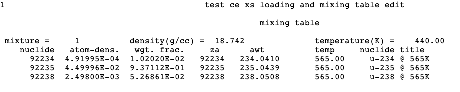
Fig. 8.1.104 Example of mixing table data for multigroup mode with DBX=0.

8.1.5.8. Albedo cross section correspondence

Printing the albedo cross section correspondence tables is optional. The headings for the tables are printed in subroutine CORRE, and then subroutine RATIO prints the data. These tables are printed only if PAX=YES is specified in the parameter data as described in Sect. 8.1.3.3. Examples of these tables are shown in Fig. 8.1.105 and Fig. 8.1.106.

The table shown in Fig. 8.1.105 contains, left to right, the cross section energy group, the lower and upper lethargy bounds, the corresponding albedo energy groups, and the cumulative probability associated with each albedo energy group for choosing the albedo energy group corresponding to the cross section energy group. The table shown in Fig. 8.1.106 is the inverse of the table shown in Fig. 8.1.105. It provides the cumulative probabilities for choosing the cross section energy group corresponding to the albedo energy group. The information in these tables is automatically generated by KENO.

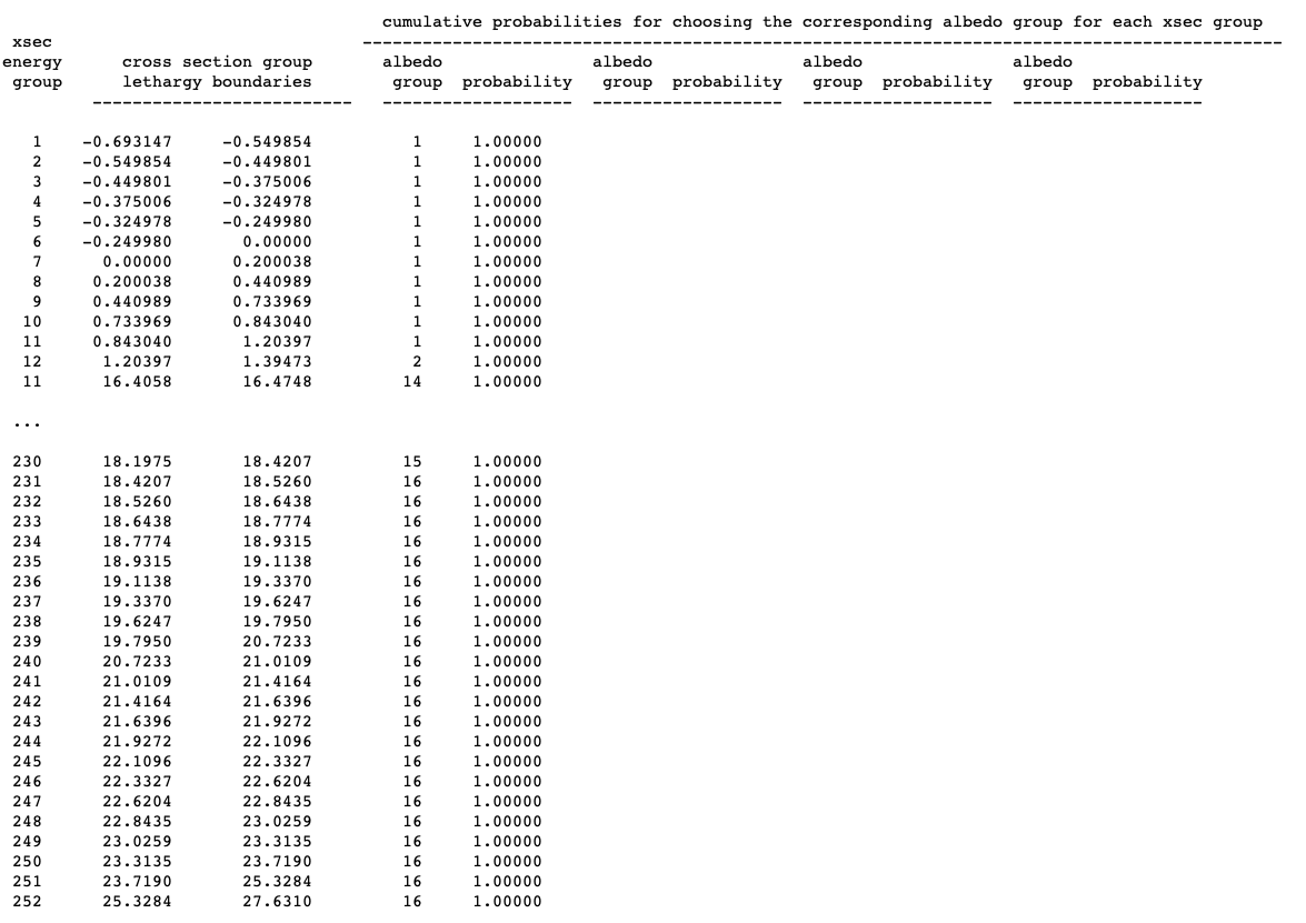
Fig. 8.1.105 Cumulative probabilities for correlating the albedo energy group to the cross section energy group.

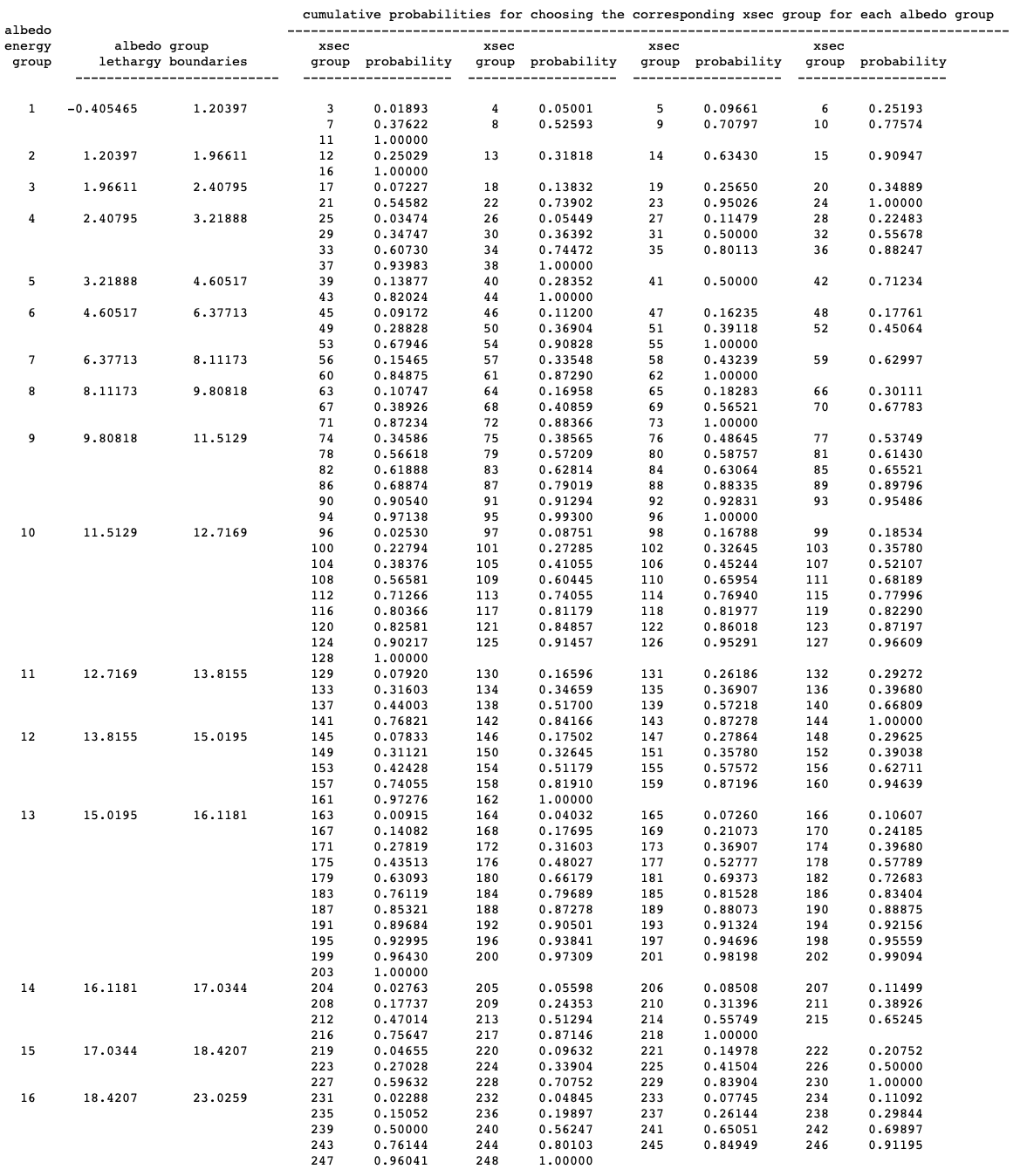
Fig. 8.1.106 Cumulative probabilities for correlating the cross section energy group to the albedo energy group.

8.1.5.9. 1-D macroscopic cross sections

The decision to print the 1-D mixture cross sections is optional. They are printed only if XS1=YES is specified in the parameter data. When the 1-D cross sections are to be printed, they are printed a group at a time for each mixture. The 1-D mixture cross sections for a mixture are shown in Fig. 8.1.107.

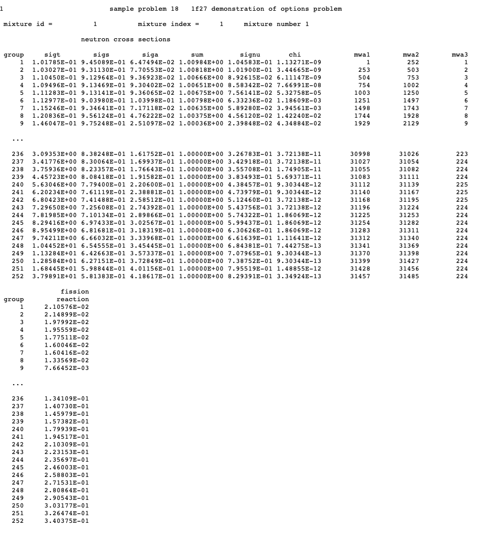
Fig. 8.1.107 Example of macroscopic 1-D cross sections.

When the 1-D mixture cross sections are printed, the problem title is printed at the top of the page. The mixture ID, mixture index, and mixture number are then printed. ID is the mixture number from the mixing table, and mixture index is the index used to reference it and mixture number is its identifier. This step is followed by a heading to identify the different 1-D cross sections. GROUP is the energy group, sigt is the total cross section for the mixture, sigs is the nonabsorption probability, siga is the absorption probability, signu is the production probability, chi is the fission spectrum, mwa1 is the pointer for the first position of the cross sections for the energy group, mwa2 is the pointer for the last position of the cross sections for the energy group, and mwa3 contains the group for the transfer corresponding to the first position. SUM is the sum of the absorption probability and the nonabsorption probability. The absorption probability is defined as the absorption cross section divided by the total cross section. The nonabsorption probability is the sum of the group-to-group transfers for this group, divided by the total cross section. The production probability is defined as the fission production cross section divided by the total cross section \(\left(v \Sigma_{f} / \Sigma_{\mathrm{T}}\right)\). The nonabsorption probability and the production probability are not true probabilities in that they may be greater than 1. This is because the nonabsorption probability has the (n,2n) transfer array summed into the total transfer array twice, and the (n,3n) is summed three times, etc.

8.1.5.10. Extra 1-d cross sections

Printing the extra 1-D cross sections is optional. They are printed if P1D=YES is specified in the parameter data. Extra 1-D cross sections are not used in KENO unless NUB=YES is specified in the parameter data or the user has altered the code to access and utilize other 1-D cross sections. If NUB=YES is specified, the extra 1-D cross section is the fission cross section, which is used to calculate the average number of neutrons per fission. This is printed only for fissile mixtures as shown in Fig. 8.1.107. The fission cross section heading follows the table of 1D cross sections. The fission cross section heading is XSEC ID 18, and it follows the table of 1-D cross sections.

8.1.5.11. 2-D macroscopic cross sections

The decision to print the 2-D mixture cross sections is optional. They are printed only if XS2=YES is specified in the parameter data. They are printed after the 1-D cross sections for the mixture. A heading is printed, followed by the transfer data. An example of the 2-D mixture cross sections is given in Fig. 8.1.108.

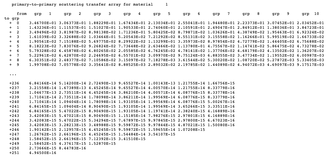
Fig. 8.1.108 Example of 2-D macroscopic cross sections.

8.1.5.12. Probabilities and angles

Printing the probabilities and angles is optional. They are printed if the number of scattering angles is greater than zero and XAP=YES is specified in the parameter data. Examples of the probabilities are shown in Fig. 8.1.109. Examples of the angles are shown in Fig. 8.1.110. If the group-to-group transfer for a mixture is isotropic, the first angle for that transfer will be set to -2.0 as a flag to the code.

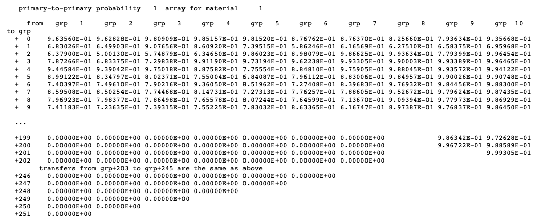
Fig. 8.1.109 Example of macroscopic probabilities.

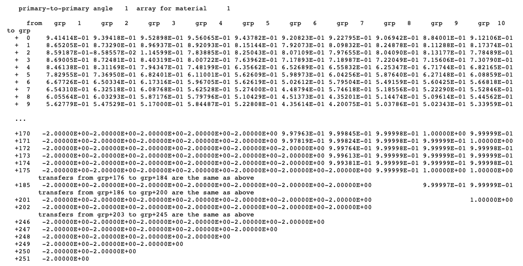
Fig. 8.1.110 Example of macroscopic angles.

8.1.5.13. Energy boundaries

KENO codes in the previous SCALE versions supported only single energy group boundaries used in all tally calculations. The energy group boundaries were obtained from the multigroup library used by transport process if the calculation mode is multigroup. These energy bounds may not be overridden by users in multigroup mode. In continuous-energy mode, energy group boundaries were defaulted to the library structure read from the SCALE 252-group multigroup library. The user could override the default energy boundaries either by defining the number of energy groups with NGP parameter, or by entering the energy points in energy data input block.

In SCALE 6.3, KENO codes can store multiple energy group boundaries; each may be used for different tallies. However, this capability is not enabled for standalone KENO calculations. If KENO is run as part of a CSAS or a TRITON sequence, then multiple energy boundaries can be entered in the definitions data input block available for these sequences (see Sect. 2.1.4.2.1).

Energy boundaries output edit always prints DEFAULT energy boundaries that are used in all tally calculations if it has not been otherwise requested. In multigroup mode, DEFAULT energy boundaries are always read from the multigroup library used by transport, and it cannot be overridden by the users. An example of energy boundaries output edit printed by a standalone multigroup KENO calculation is given in Fig. 8.1.111.

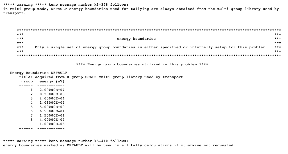
Fig. 8.1.111 Example of energy boundaries output edit for multi group mode.

In continuous-energy mode, DEFAULT energy boundaries are defaulted to the library group structure of the SCALE 252-group library and can be overridden by (1) setting the number of energy groups with NGP parameter as shown in Example 8.1.44 and Example 8.1.45, (2) entering all energy points in energy data block Example 8.1.46, or (3) entering energy boundaries in the definitions data block (valid when running KENO codes as part of a sequence, see Sect. 2.1.4.2.1 for more details).

Example 8.1.44 Energy boundaries are set by NGP=11

...

read parameter
   ...
   NGP=11
end parameter

...

Example 8.1.45 Energy boundaries are set by NGP=8

...

read parameter
   ...
       NGP=8
end parameter

...

Example 8.1.46 Energy boundaries are read from energy data block

...

read energy
   2.e7 1.e5 1.e1 0.65 1.e-4
end energy

...

Three examples of energy boundaries output edits for continuous-energy KENO calculations are given in the Fig. 8.1.112, Fig. 8.1.113, and Fig. 8.1.114. In the first example, the energy boundaries constructed with having 11 equal lethargy intervals by setting NGP=11 overwrites the DEFAULT energy boundaries. Fig. 8.1.113 shows the energy group output edits for a case in which the DEFAULT energy boundaries are overridden by the energy boundaries read from the SCALE 8 group test library that was provided by setting NGP=8. And the DEFAULT energy boundaries are overridden in the last example whose output edit shown in Fig. 8.1.114 by reading the energy boundaries from the energy data input block.

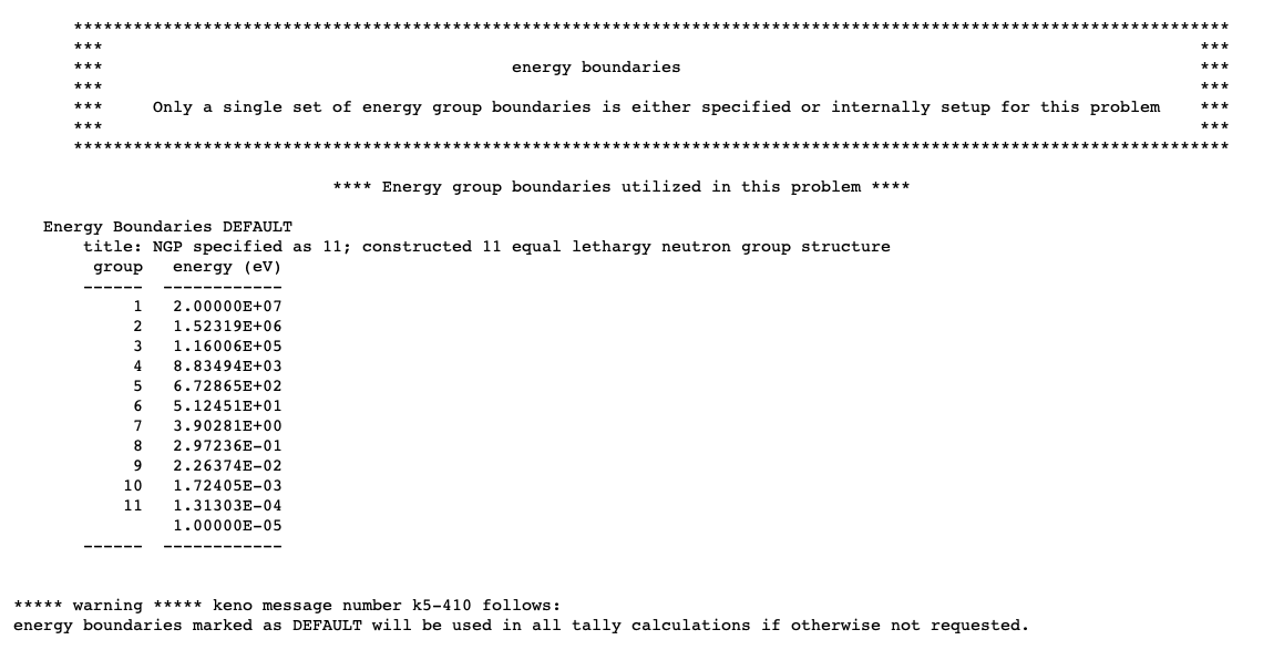
Fig. 8.1.112 Example of energy boundaries output edit for continuous-energy mode (NGP=11).

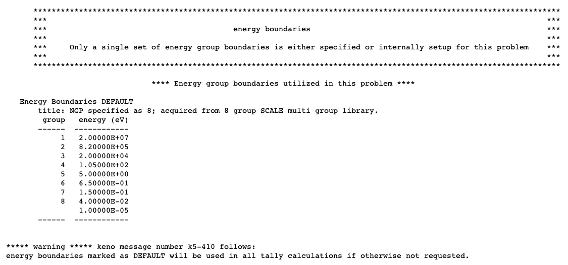
Fig. 8.1.113 Example of energy boundaries output edit for continuous-energy mode (NGP=8).

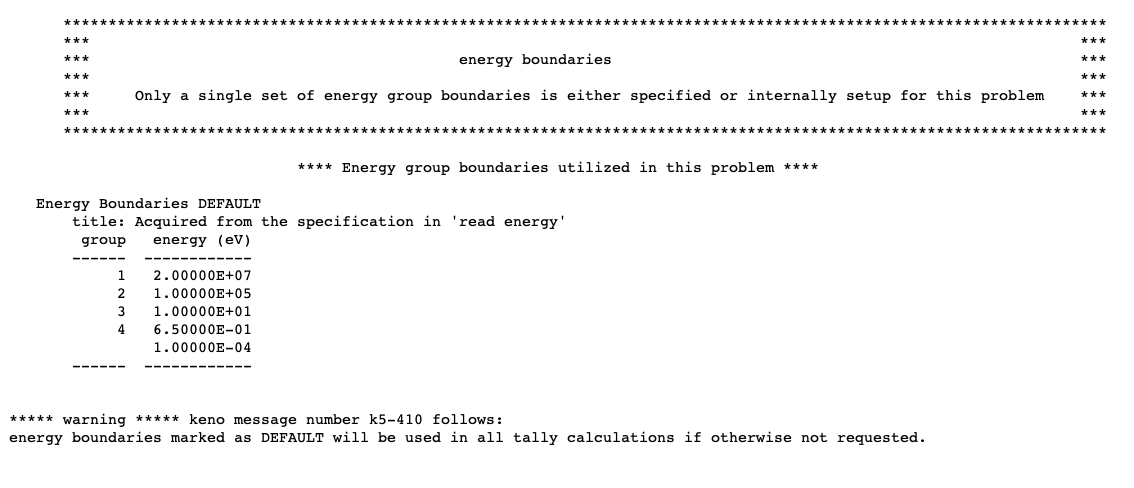
Fig. 8.1.114 Example of energy boundaries output edit for continuous-energy mode (energy data).

8.1.5.14. Array summary

The arrays that are used in the problem are summarized in the table shown in Fig. 8.1.115. This table is printed whenever more than one array is used in the problem.

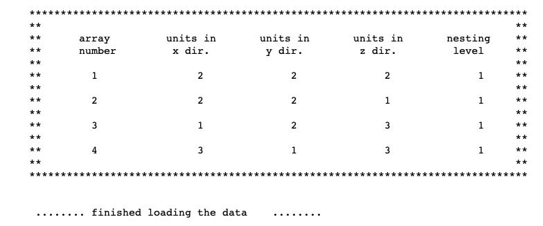
Fig. 8.1.115 Example of array summary.

The ARRAY NUMBER is the number by which the array is designated in the input data. The number of units in the X, Y, and Z directions is listed for each array. The NESTING LEVEL indicates the level of nesting for each array. The global, overall, or universe array is flagged by the word GLOBAL. The global array should always appear at the first nesting level. Arrays that have been placed in the global reflector by using holes should also appear at the first nesting level. A nesting level of one is the highest or first nesting levels. The larger the number in the nesting level column, the deeper the nesting level will be.

8.1.5.15. Geometry data edits

8.1.5.15.1. KENO V.a geometry edit

The geometry region data used by the problem are always printed and cannot be suppressed. They should be carefully examined by the user to verify the mixture number, bias ID, and geometry specifications used in the problem. If geometry region data are entered but are not referenced in the unit orientation array data, they will not be printed here. An example would be to enter geometry region data describing Units 1, 2, 3, and 4 and to use only Units 1, 3, and 4 in the unit orientation array. Then the geometry region data for Unit 2 will not be printed. An example of the KENO V.a geometry region printout for a problem is given in Fig. 8.1.116.

The problem title and a heading are printed at the top of each page. REGION is the region number within a unit. Each unit has its regions numbered sequentially, beginning with one. MEDIA NUM is the mixture number or mixture ID that occupies the volume defined by the region. BIAS ID is the bias ID that corresponds to the desired set of weight average for biasing the region. The unit number is printed at the top of each unit’s geometry region description near the center of the page. The data printed for each geometry region include (1) the region number relative to the unit (numbered sequentially within the unit), (2) the shape of the geometry region, (3) the mixture ID of the material within the volume defined by the region, (4) the bias ID to define the average weight of a neutron in the region, and (5) the dimensions defining the outer boundaries of the geometry region. If additional geometry surrounds an array, a heading is printed stating: UNIT ____ EXTERNAL TO LATTICE ____. The lattice number is the number of the array that is surrounded by the specified geometry. The unit number is the unit that contains the specified geometry. In the case of an external reflector for the global array, the unit number is assigned by the code.

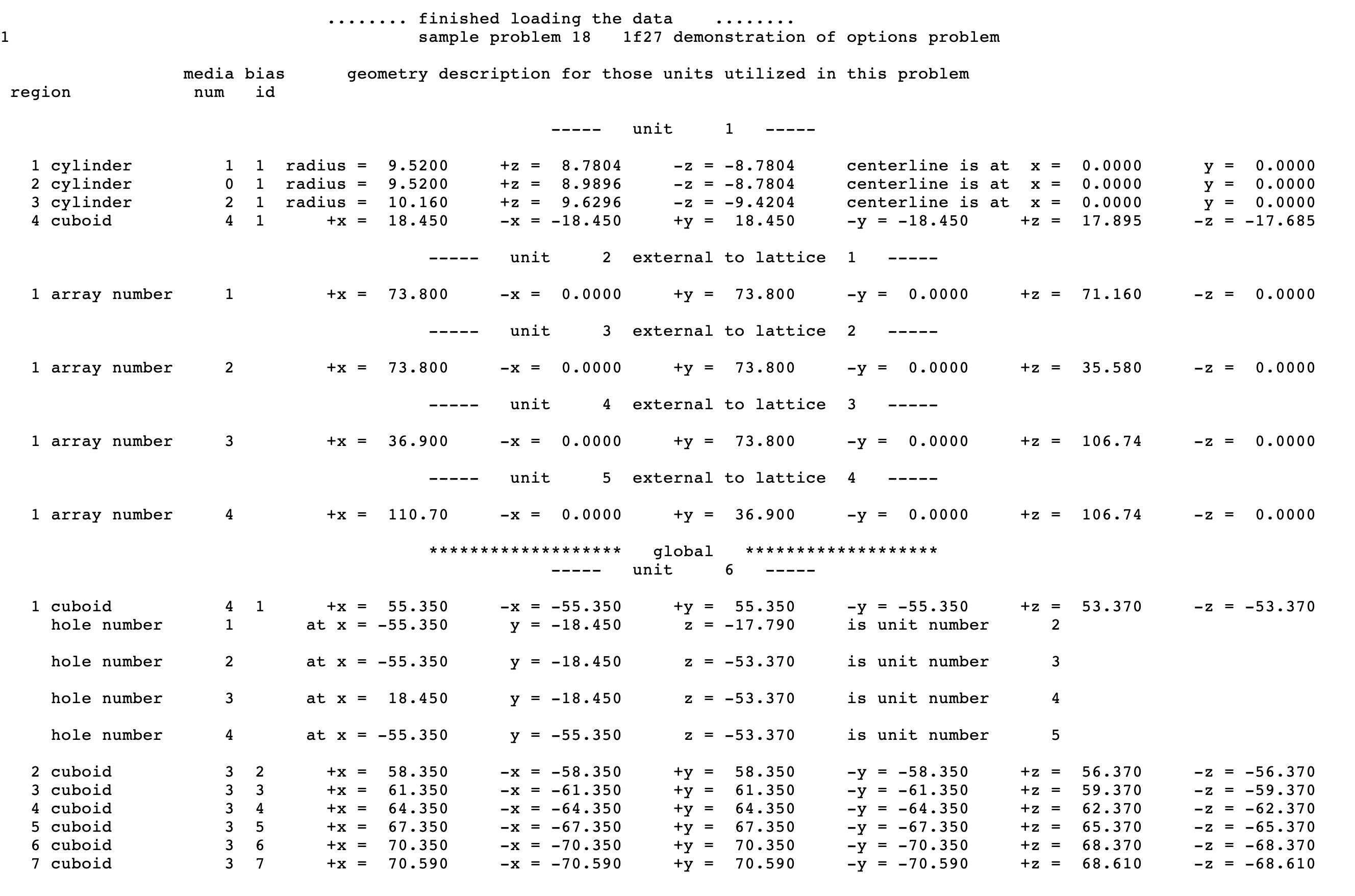
Fig. 8.1.116 Example of KENO V.a geometry region data

8.1.5.15.2. KENO-VI geometry edit

The geometry region data utilized by the problem are printed and cannot be suppressed. They should be carefully examined by the user to verify the mixture number, bias ID, and geometry specifications used in the problem. If geometry region data are input but are not referenced in the unit orientation array data, they will not be printed here. An example would be to input geometry region data describing Units 1, 2, 3, and 4 and to utilize only Units 1, 3, and 4 in the unit orientation array. Then the geometry region data for Unit 2 will not be printed. An example of the geometry region printout for a problem is given in Fig. 8.1.117 and Fig. 8.1.118.

First, a table of geometry parameters for the problem is printed. This specifies the overall size of the problem, number of components in the problem, and the size of the array needed to store the geometry. Next, the quadratic equations by unit are printed. The problem title and a heading are printed at the top of each page. The unit number followed by the GEOMETRY data for that unit is then printed. Each geometry record type used in the unit, numbered in the order they appear in the unit, is printed out. Following each geometry record type is the set of quadratic equations that describe the input geometry for that geometry record. The CONTENTS data, consisting of four columns, are then listed in the order they appear in the problem. The first column contains the content keyword. The second column contains the media/hole/array number. The third column labeled IMP contains the bias ID number if the content keyword is MEDIA. Otherwise, this column is blank. The fourth column contains the sector definition array, which describes the region location relative to the GEOMETRY records listed above for that unit.

The data consisting of the unit number, GEOMETRY data, and CONTENT data are repeated for each unit used in the problem. The global unit has a heading printed before the unit number to identify it as the global unit.

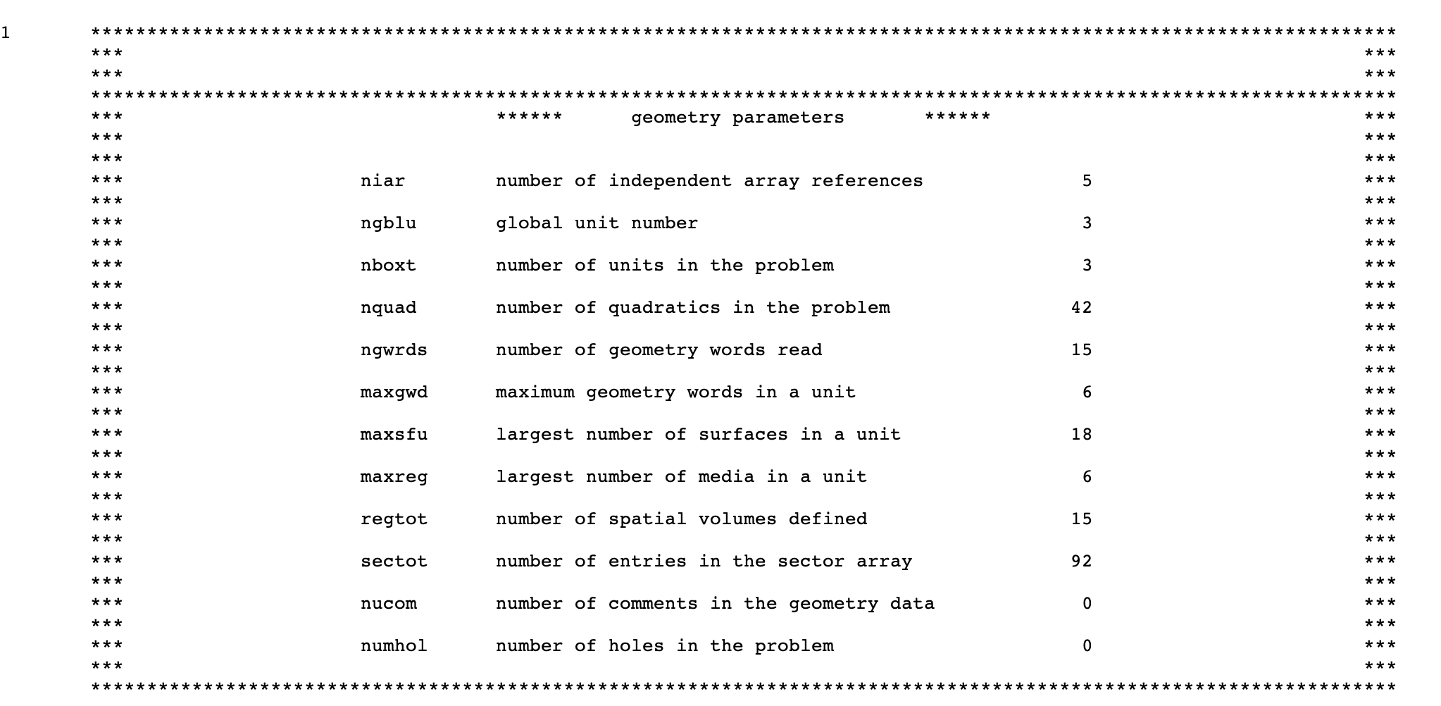
Fig. 8.1.117 Example of KENO-VI geometry parameter table.

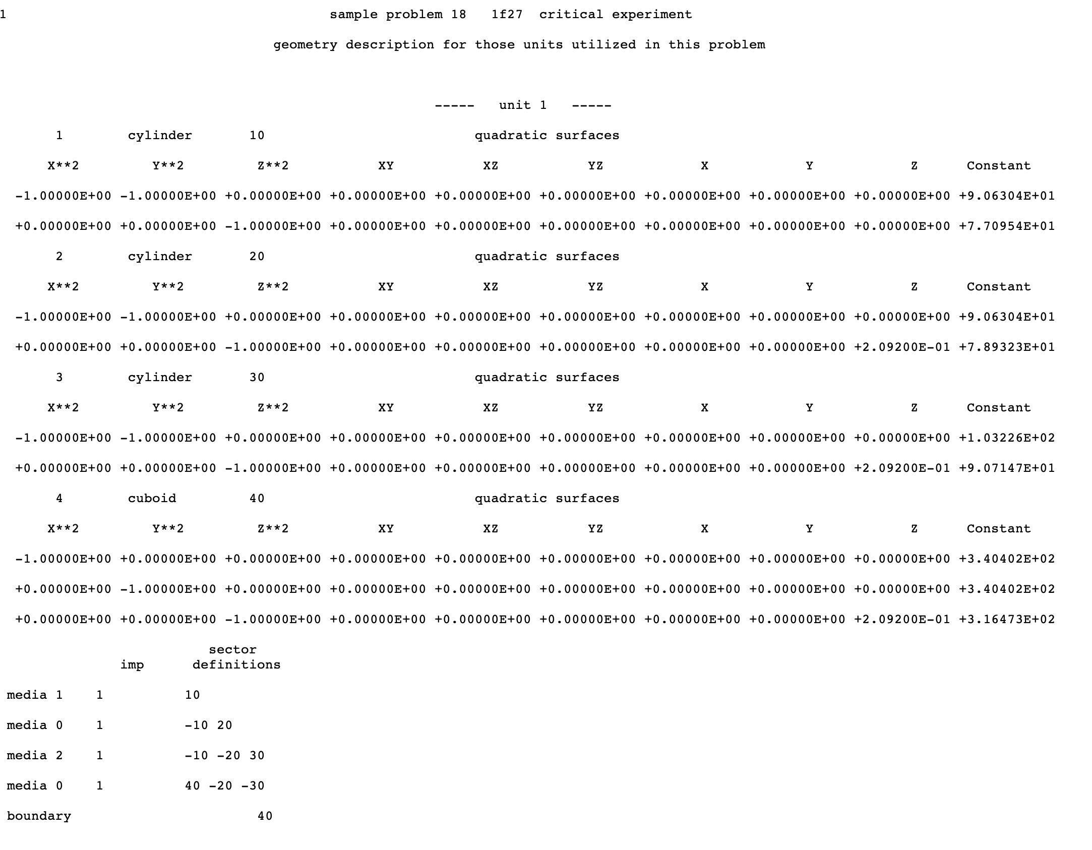
Fig. 8.1.118 Example of KENO-VI geometry region data.

8.1.5.16. Unit orientation description

Each unit orientation description defines the location of units in the 3-D lattice that represent the specified array. The array described is identified in the heading UNIT ORIENTATION DESCRIPTION FOR ARRAY ____. The arrays used in the problem are stacked together to represent the physical problem being analyzed. The unit orientation description is not printed if only Unit 1 is described in the problem. The user should carefully examine the unit orientation descriptions to ensure proper placement of the units in each lattice. A sample unit orientation description is shown in Fig. 8.1.119 .

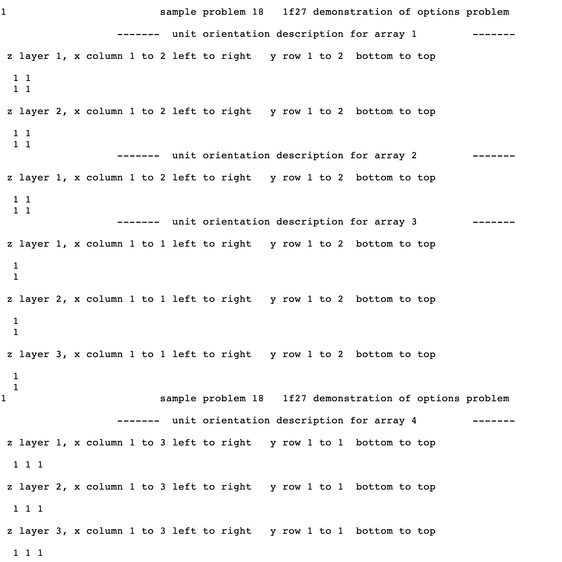
Fig. 8.1.119 Example of unit orientation description.

If a very large array is used by the problem, its unit orientation description may be spread over several pages. When checking the printout, the user should pay careful attention to the headings that indicate the portion of each lattice being printed. The detailed printout of an array may be suppressed using the ARRAY parameter PRT=no.

8.1.5.17. Volume information

The volume information printout differs between KENO V.a and KENO-VI. Because it does not allow intersections of bodies, KENO V.a is always able to calculate analytically the volume of any region in the geometry. KENO-VI, on the other hand, never calculates volumes analytically. In fact, KENO-VI never calculates volumes unless it is directed to do so, but it can read volumes off the MEDIA cards or off a VOLUME file (Sect. 8.1.3.13).

8.1.5.17.1. KENO V.a volume edit

Three tables of volumes are always printed and cannot be suppressed. The problem title is printed at the top of the page, followed by the heading “VOLUMES FOR THOSE UNITS UTILIZED IN THIS PROBLEM.” An example of the volume printout is given in Fig. 8.1.120.

The first table is arranged by ascending unit number. It includes (1) the unit number, (2) the region number within the unit, (3) the overall geometry region number, (4) the net volume of each individual region, and (5) the cumulative volume through each region in the unit. The cumulative volume of the last region in a unit is the total volume of the unit. The unit number is printed under the heading UNIT. Data listed under the heading REGION refer to the number of the geometry region within the unit. The geometry regions within a unit are numbered sequentially starting with 1. Data entered under the heading GEOMETRY REGION refer to the entry number of the individual geometry region. These are numbered sequentially, starting with 1, through the TOTAL INPUT GEOMETRY REGIONS defined in Fig. 8.1.120. The net volume of each individual region is calculated by subtracting the volume of the interior region from the volume of the region and is listed under the heading VOLUME. The data listed under the heading CUMULATIVE VOLUME are calculated from the dimensions of the region. A simple example demonstrating how volumes are calculated can be given by assuming a unit that is composed of three concentric cubes. Region 1 is a cube 3 cm on a side, region 2 is a cube 4 cm on a side, and region 3 is a cube 5 cm on a side. The cumulative volume of region 1 is 27 cm³ (3³); the cumulative volume of region 2 is 64 cm³ (4³); the cumulative volume of region 3 is 125 cm³ (5³). The volume of region 1 is 27 cm³ (3³), the volume of region 2 is 37 cm³ (64 - 27), and the volume of region 3 is 61 cm³ (125 - 64).

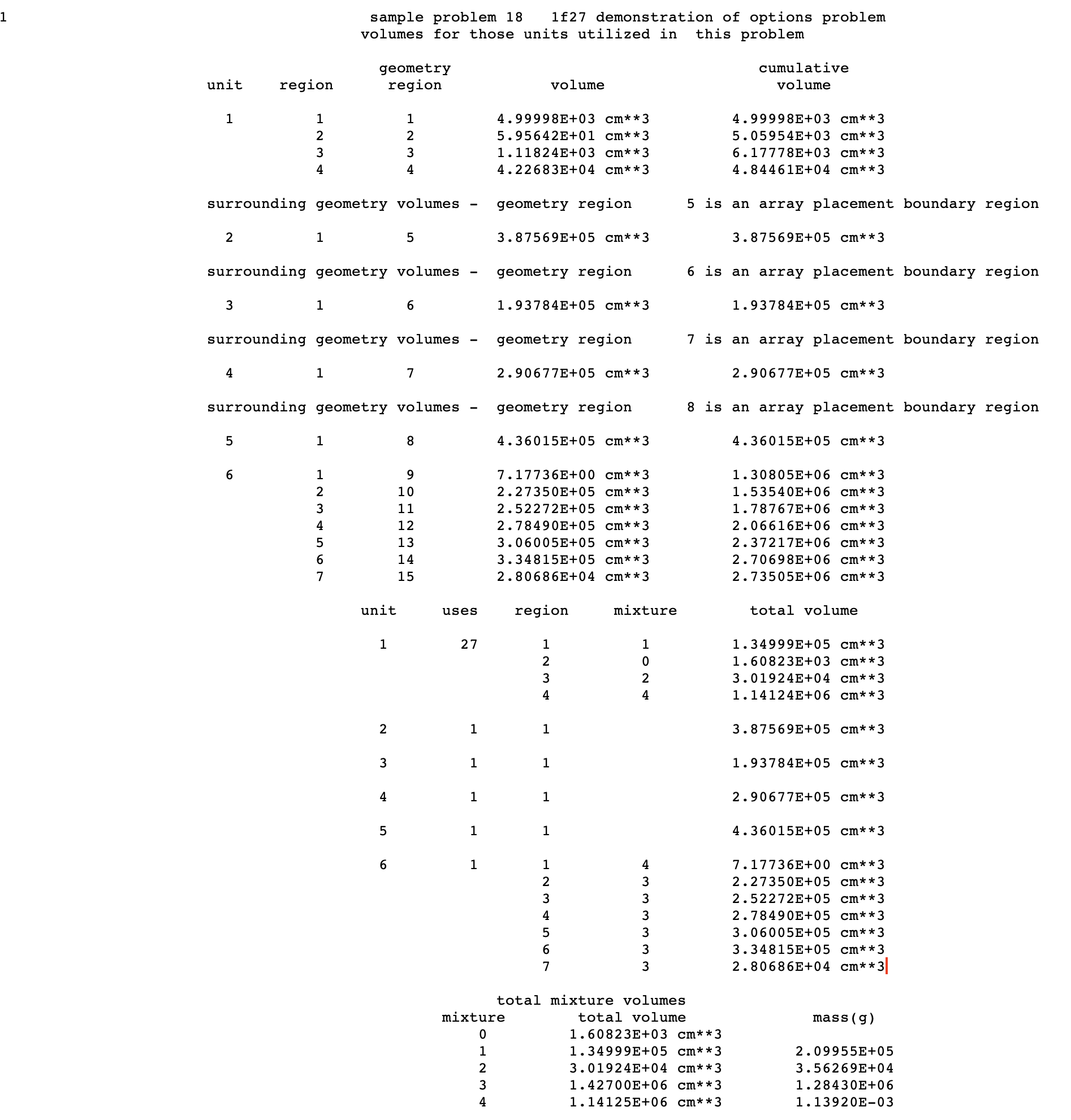
Fig. 8.1.120 Sample volume information.

The second table contains (1) the unit number, (2) the number of times the unit is used in the problem, (3) the region number within the unit, (4) the mixture number present in the region, and (5) the total volume associated with the region in the whole problem. The unit number is printed under the heading UNIT, data printed under the heading USES indicates the number of times the unit is used in the problem. Data printed under the heading MIXTURE indicates the mixture number used in the region. The total volume of each region is printed under the heading TOTAL VOLUME and is determined by multiplying the VOLUME of the region listed in the first table by the number of times the unit containing that region is used in the problem.

The third table is printed following the heading “TOTAL MIXTURE VOLUMES.” In this table, the mixtures used in the problem are listed with their associated total volume and total mass. The mixture numbers are printed under the heading MIXTURE, the total volume of each mixture is printed under the heading TOTAL VOLUME, and the mass of each mixture is printed under the heading MASS(G). All masses will be printed as zero if the working format cross section library does not contain the data required to calculate the densities of the mixtures used in the problem.

8.1.5.17.2. KENO-VI volume edit

Two tables of volumes are printed by subroutine VOLUME and cannot be suppressed. The first table will list the number of times each unit is used in the problem and the total volume of each region throughout the entire problem description. The second table will list the total volume and mass of each mixture used in the problem.

If a volume calculation type of NONE is specified and no volumes are read in for the regions, then the volumes will be set to -1.0, which will result in negative fluxes and fission densities. A sample volume output edit for such a case is given in Fig. 8.1.121. Calculations with zero volumes always provide a notification with a warning message as shown in Fig. 8.1.121.

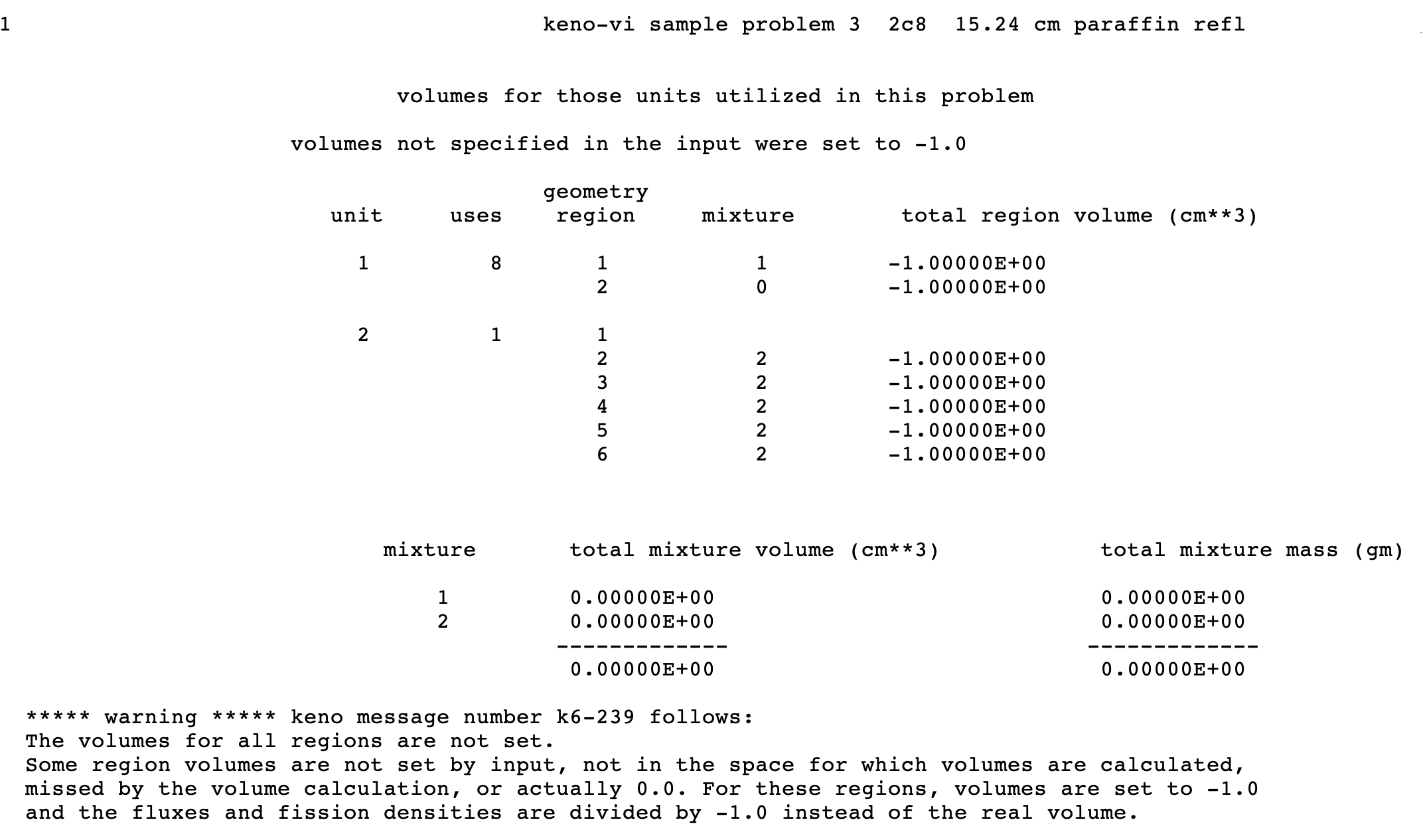
Fig. 8.1.121 Sample volume information (volumes are neither defined nor calculated).

For the calculated volumes, an error estimate is printed after the volumes. A summary of the parameters used in both TRACE and RANDOM volume estimates and some diagnostic information is always printed before the first table if any region volume is calculated by one of these methods. Two examples of the KENO-VI volume output edits with these volume calculation methods are given in Fig. 8.1.122 and Fig. 8.1.123, respectively.

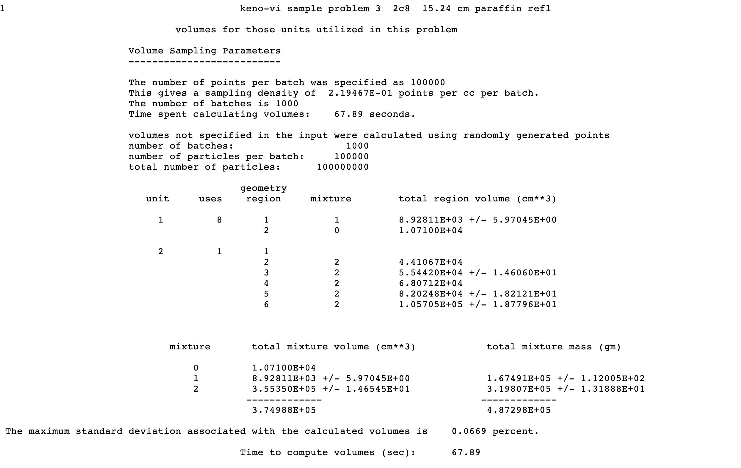
Fig. 8.1.122 Sample volume information, undefined volumes are calculated by RANDOM estimate.

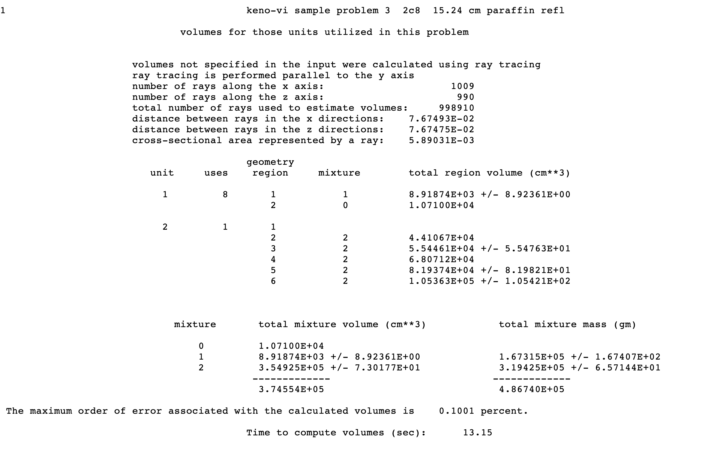
Fig. 8.1.123 Sample volume information, undefined volumes are calculated by TRACE estimate.

The unit number is printed under the heading UNIT. The REGION refers to the number of the geometry region within the unit determined by the order of the CONTENT records in the unit. USES indicates the number of times the unit is used in the problem. MIXTURE is the mixture number used in the region. A blank indicates an array or unit, placed in a hole, in that region. TOTAL VOLUME is the total volume of that region followed by +/- and an error estimate if the volume for the region was calculated.

If mesh volumes are used, there will be a table listing the cumulative volumes generated by summing the mesh volumes, the deviations, and the deltas between the summed volumes and the overall volumes for the regions. If the overall volume has been calculated, then the delta should be zero, but if it was entered, then the delta will show the difference.

In the last table, the mixtures used in the problem are listed along with their total volumes and masses. Along with the total volumes and masses, an error estimate is printed for any mixtures having regions that were calculated using either the RANDOM or TRACE volume estimates..

8.1.5.18. Mesh volumes output edit

With the mesh flux accumulator, fluxes are tabulated for each region of each unit in the defined mesh grid. KENO computes the volume of each region in each mesh interval so that fluxes per unit volume can be determined. For KENO V.a models where the mesh flux accumulator is activated by setting MFX=YES and either (a) the mesh size set to a positive value with MSH=, or (b) mesh grid defined by grid geometry data input, a mesh volume sampling summary and the cumulative volume of all mesh intervals for a given region are printed as shown in Fig. 8.1.124. Details of mesh grid 20001 on which a mesh volume calculation was performed are printed in the grid definitions output edit. An example of grid definitions output edit can be shown in Sect. 8.1.5.19.

Note that KENO V.a allows users to alter the default settings for the mesh volume calculation. However, TRACE volume estimate is not available for mesh volume; therefore, the RANDOM volume estimate is always enforced when type=trace is entered in volume data. A corresponding warning message (message number k?=370) is printed in the output to notify the user about this change.

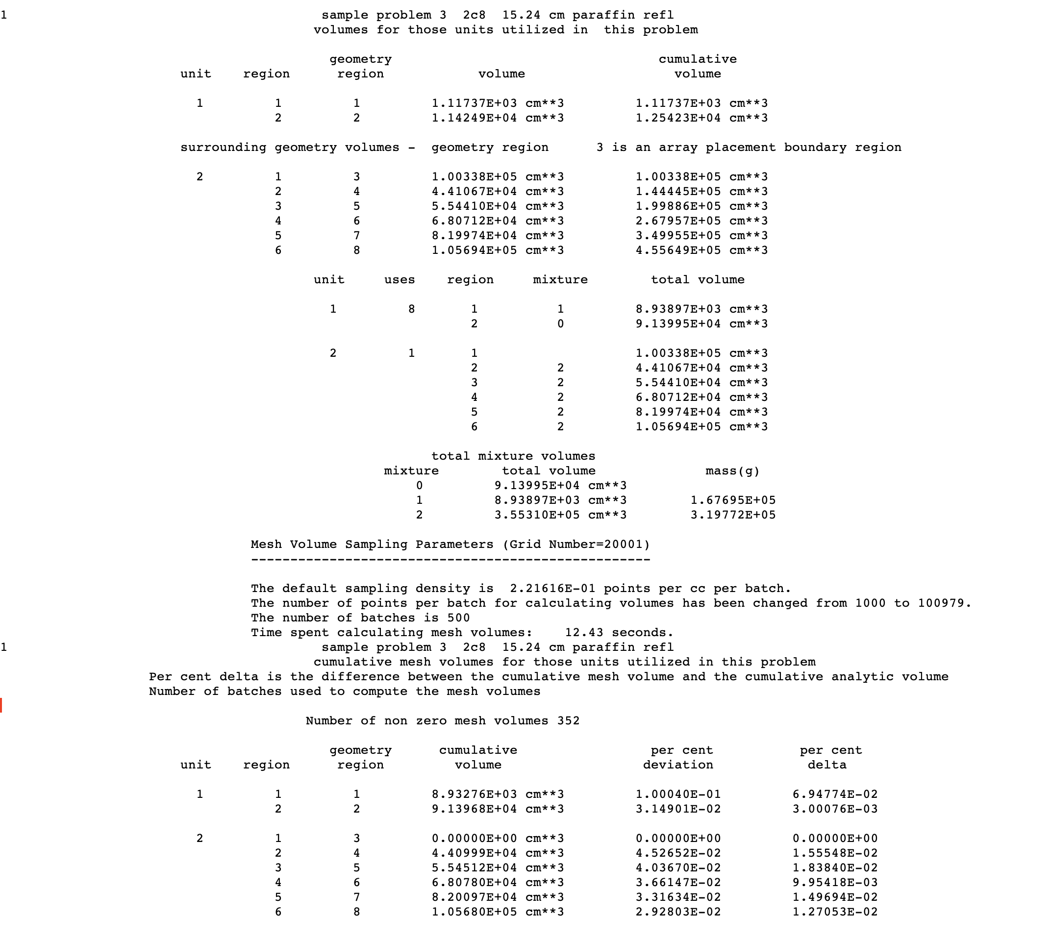
Fig. 8.1.124 Sample sum of mesh volumes edit (KENO V.a with cubic mesh, MSH=20.0).

Note

Unlike the KENO V.a implementation, mesh flux accumulation with KENO-VI always needs a volume data input block to activate the mesh volume calculation; otherwise, calculation is terminated with an error message. KENO-VI does not support mesh volume calculation with TRACE volume estimation. Just as KENO V.a does, KENO-VI continues by using the RANDOM volume estimation for the mesh volume calculation.

An optional edit of volumes for each mesh interval for each region can be activated by entering PMV=YES in the parameter input. This edit can be very large, especially if a small mesh size is used with a large model. A sample of the volume by mesh for each region is shown in Fig. 8.1.125.

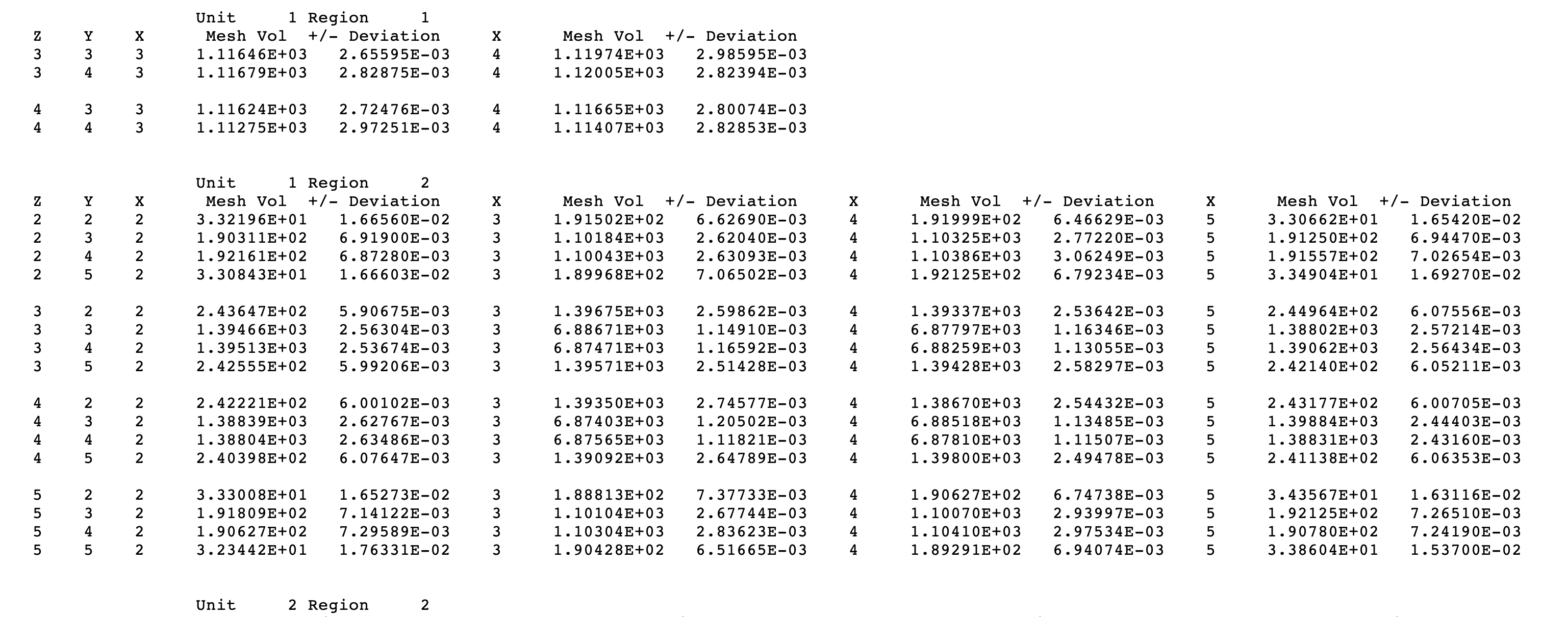
Fig. 8.1.125 Sample of volume by mesh for each region (only a small section of the output).

8.1.5.19. Grid definitions

This table specifies the mesh grids to be used in the problem. Each mesh grid is either defined by the MSH parameter and/or grid geometry data input, or constructed internally. An example of grid information is given in Fig. 8.1.126.

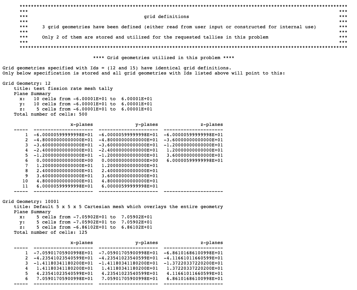
Fig. 8.1.126 Sample of grid definitions.

Grid definitions output edit lists all user-defined and internally constructed mesh grids, even some that are not used for any mesh tally. Only one of the grids is stored in the grid data container if the multiple grids are defined with identical grid data. This can be easily seen in the diagnostic messages followed by grid definitions header as well as the messages printed just before each stored grid entry. The sample grid definitions shown in Fig. 8.1.126 specify that two mesh grids with grid IDs= 12 and 15 were defined by two grid geometry data inputs, but only one of them was stored since their definitions were identical. A default mesh grid was also shown in Fig. 8.1.126 that was constructed for Shannon entropy tallies.

8.1.5.20. Biasing information

This table specifies the weighting or biasing data to be used in the problem. An example of biasing information is given in Fig. 8.1.127.

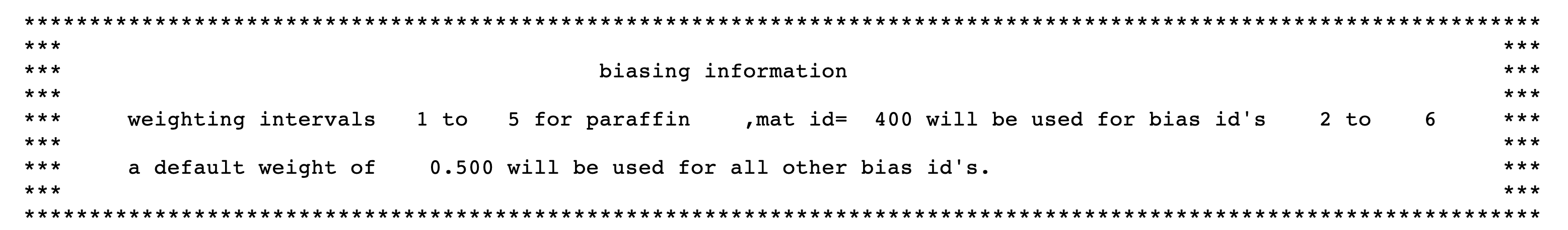
Fig. 8.1.127 Biasing information.

The user is responsible for determining from the input data whether the group-dependent weights (wtavg) for the specified material(s) were obtained from the weighting library or were entered by the user. The group-dependent weights can be printed for verification purposes as shown in Sect. 8.1.5.21.

8.1.5.21. Group-dependent weights

Printing the group-dependent weights is optional. They are printed if PWT=YES is entered in the parameter data. An example of the printed group-dependent weights is shown in Fig. 8.1.128.

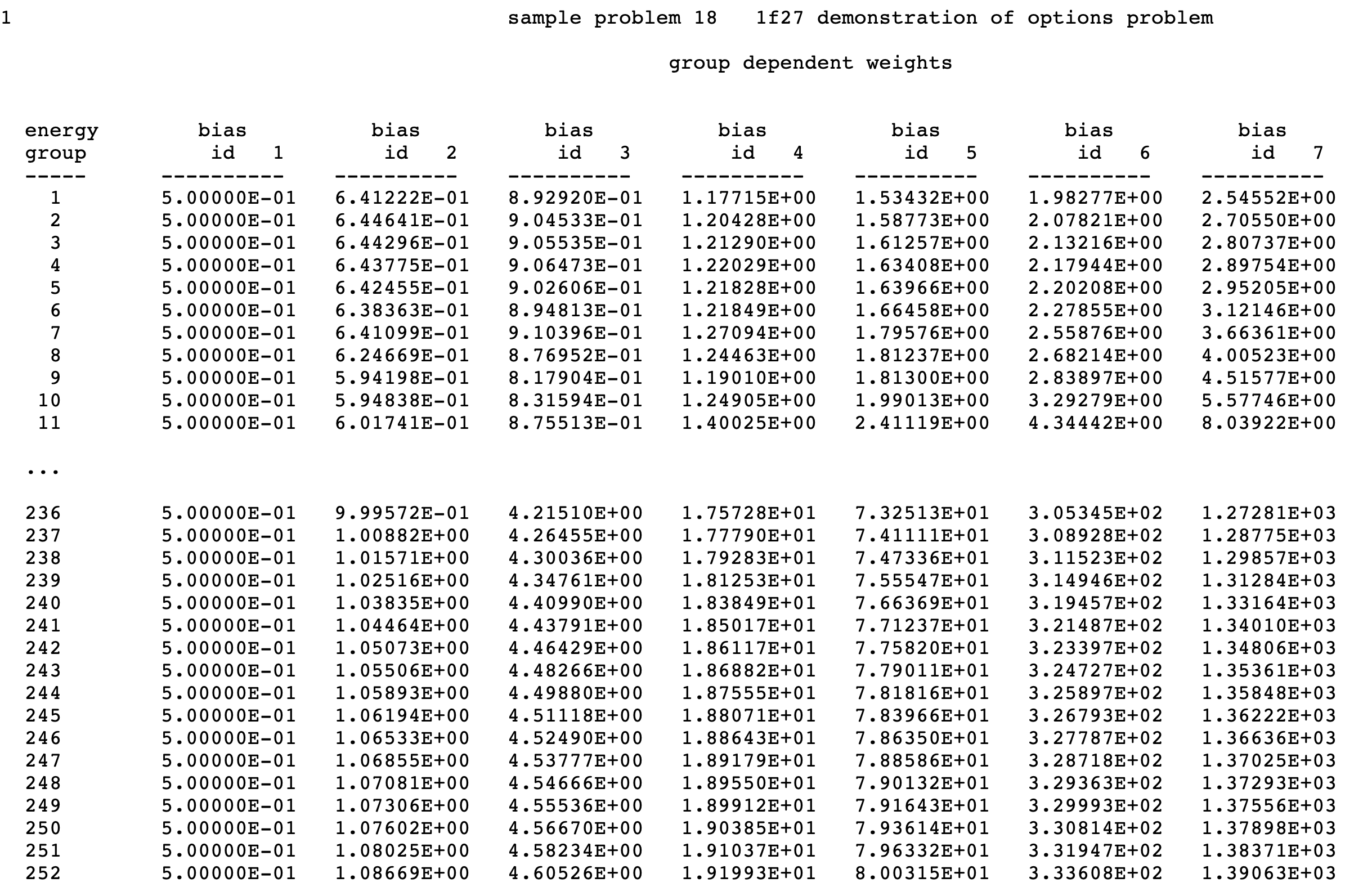
Fig. 8.1.128 Example of biasing data.

The title is printed at the top of the table. The average weight (wtavg) is printed for each energy group and each BIAS ID. The BIAS ID number printed at the top of the column corresponds to the BIAS ID used in the geometry region description or MEDIA record and printed in the biasing information.

8.1.5.22. Plot representation

Plots representing 2-D slices through the geometrical description of the problem are optional. They are created if plot data are entered unless PLT=NO is specified either in the plot data or the parameter data. Plots can be generated and displayed as (1) character plots with alphanumeric characters representing mixture numbers, unit numbers, or bias ID numbers or (2) color plots with colors representing mixture numbers, unit numbers, or bias ID numbers. Color plots generate a PNG file and require an independent program to be displayed.

An example of the output generated using the character plot method is given in Fig. 8.1.129 and Fig. 8.1.130. An example of the output generated using the color plot method is given in Fig. 8.1.131 and Fig. 8.1.132.

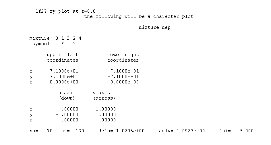
Fig. 8.1.129 Summary of character plot symbols, coordinates, and data.

Fig. 8.1.129 summarizes the data used to generate the character plot. Fig. 8.1.130 is an example of a character plot of the 2-D slice specified through the geometrical description of the problem. In Fig. 8.1.129, the plot title is printed at the top of the page, followed by a statement that “THE FOLLOWING WILL BE A CHARACTER PLOT.” If a plot title was not entered in the plot data, the plot title is defaulted to the problem title. The title is followed by a heading specifying the type of plot (MIXTURE MAP, BIAS ID MAP, or UNIT MAP). This is followed by a table that correlates the symbols to be used in the character plot with the mixture numbers, bias ID numbers, or unit numbers that were used in the problem. If the problem is a bare array, the overall system coordinates are printed. Then the coordinates of the upper left corner and lower right corner of the plot are printed. This is followed by the direction cosines down and across the plot. The remaining plot parameters (including both input data and calculated values) are then printed. NU is the number of characters printed in the U (down) direction, NV is the number of characters printed in the V (across) direction, DELU is the incremental distance, in cm, represented by each character in the U (down) direction, DELV is the incremental distance, in cm, represented by each character in the V (across) direction, and LPI is the vertical to horizontal scaling factor for plot proportionality.

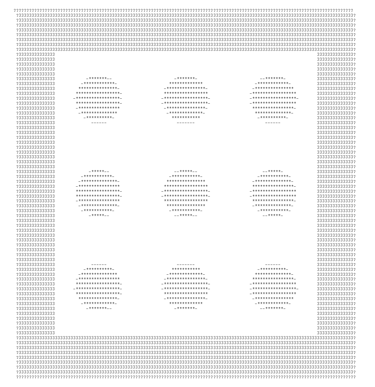
Fig. 8.1.130 Sample character plot representation.

Fig. 8.1.130 shows a character plot of a 2-D slice specified through the geometrical description of the problem. These plots aid the user in verifying that the problem is described correctly. Any number of plots can be made in one problem.

Fig. 8.1.131 summarizes the data used to generate the color plot. Fig. 8.1.132 is an example of a color plot of the 2-D slice specified through the geometrical description of the problem. This plot does not appear in the KENO printout. It is generated from a PNG file that is created when a color plot has been specified in the KENO input data and requires special processing by the user.

In Fig. 8.1.131, the plot title is printed at the top of the page, followed by a statement that “THE FOLLOWING WILL BE A COLOR PLOT.” If a plot title was not entered in the plot data, the plot title is defaulted to the problem title. The title is followed by a heading specifying the type of plot (MIXTURE MAP, BIAS ID MAP, or UNIT MAP). If the problem is a bare array, the overall system coordinates are printed. Then the coordinates of the upper left corner and lower right corner of the plot are printed. This is followed by the direction cosines down and across the plot. The remaining plot parameters (including both input data and calculated values) are then printed. NU is the number of characters printed in the U (down) direction, NV is the number of characters printed in the V (across) direction, DELU is the incremental distance, in cm, represented by each character in the U (down) direction, DELV is the incremental distance, in cm, represented by each character in the V (across) direction, and LPI is the vertical to horizontal scaling factor for plot proportionality.

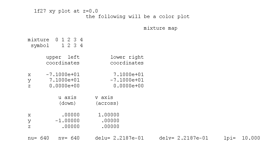
Fig. 8.1.131 Summary of color plot symbols, coordinates, and data.

Fig. 8.1.132 shows an example of a color plot of a 2-D slice specified through the geometrical description of the problem. Any number of plots can be made in one problem. The color plots can be valuable tools to assist the user in verifying that a problem is described correctly.

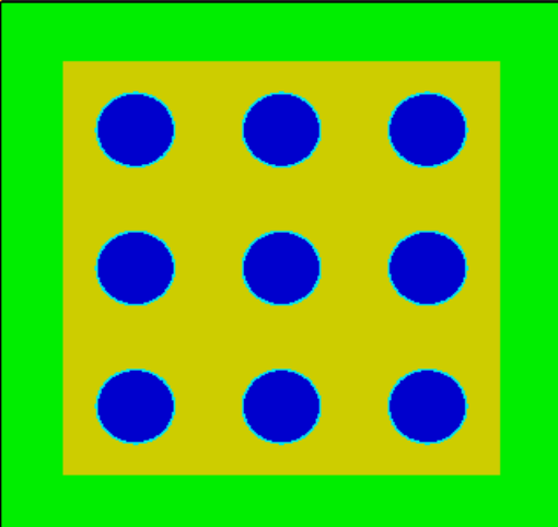
Fig. 8.1.132 Sample color plot representation.

8.1.5.23. Initial source and final pretracking edits

Prior to calculating the keff values for each generation, KENO prints the number of I/Os used before tracking and the number of minutes used processing the data. If the problem is not a restart problem, initial source information follows those two lines as shown in both Fig. 8.1.133 (KENO V.a example) and Fig. 8.1.134 (KENO-VI example).

The VOLUME FRACTION OF FISSILE MATERIAL IN THE SYSTEM is the first line of data printed for KENO V.a case. This is followed by the start type, other data used to generate the initial source distribution, and finally, the amount of time used to generate the initial source distribution and the total elapsed time. Fig. 8.1.133 illustrates starting information printed for start type 0. The cuboid for choosing starting points is (1) the bounding box around the global array (either bare or reflected) (2) the overall system if the outermost region is a cuboid, or (2) a cuboid specified by the user via the keywords XSM=, XSP=, YSM=, YSP=, ZSM=, and ZSP=.

Fig. 8.1.133 illustrates typical starting data for start type 0 (a flat start in fissile material). The parameter used in this example was NST=0.

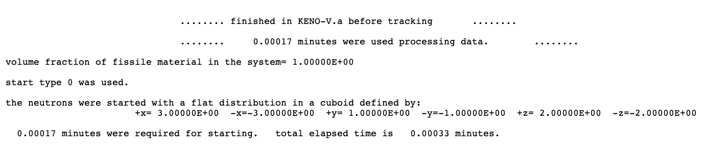
Fig. 8.1.133 Example of initial source information for start type 0 (KENO V.a).

In KENO-VI case, the first line is a warning message followed by the VOLUME FRACTION OF FISSILE MATERIAL IN THE SYSTEM line. This warning message notifies users about the potential issues that might be encountered when the volume fraction of fissile material in the system is calculated, especially for the cases in which volumes are partially defined or computed. In such cases, the volume fraction of fissile could be a negative values since KENO-VI resets the undefined volumes to -1.0.

This message is followed by the start type, other data used to generate the initial source distribution, and finally, the amount of time used to generate the initial source distribution and the total elapsed time. Fig. 8.1.134 illustrates the starting information printed for start type 0.

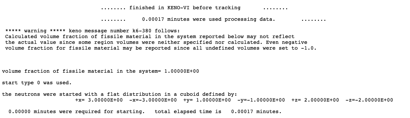
Fig. 8.1.134 Example of initial source information for start type 0 (KENO-VI).

8.1.5.24. Reference center for flux moment/angular flux transform

When TFM=YES is entered, the flux moments and angular fluxes are computed in a transformed coordinate system, relative to a “reference center” point. The default position for the reference center is the center of all fueled regions in the model. However, the center can be specified by the user for each region defined in the system model using the “center” modifier on a region input card. Edits of the fuel center and the position of the reference center for each region are shown when TFM=YES as shown in Fig. 8.1.135.

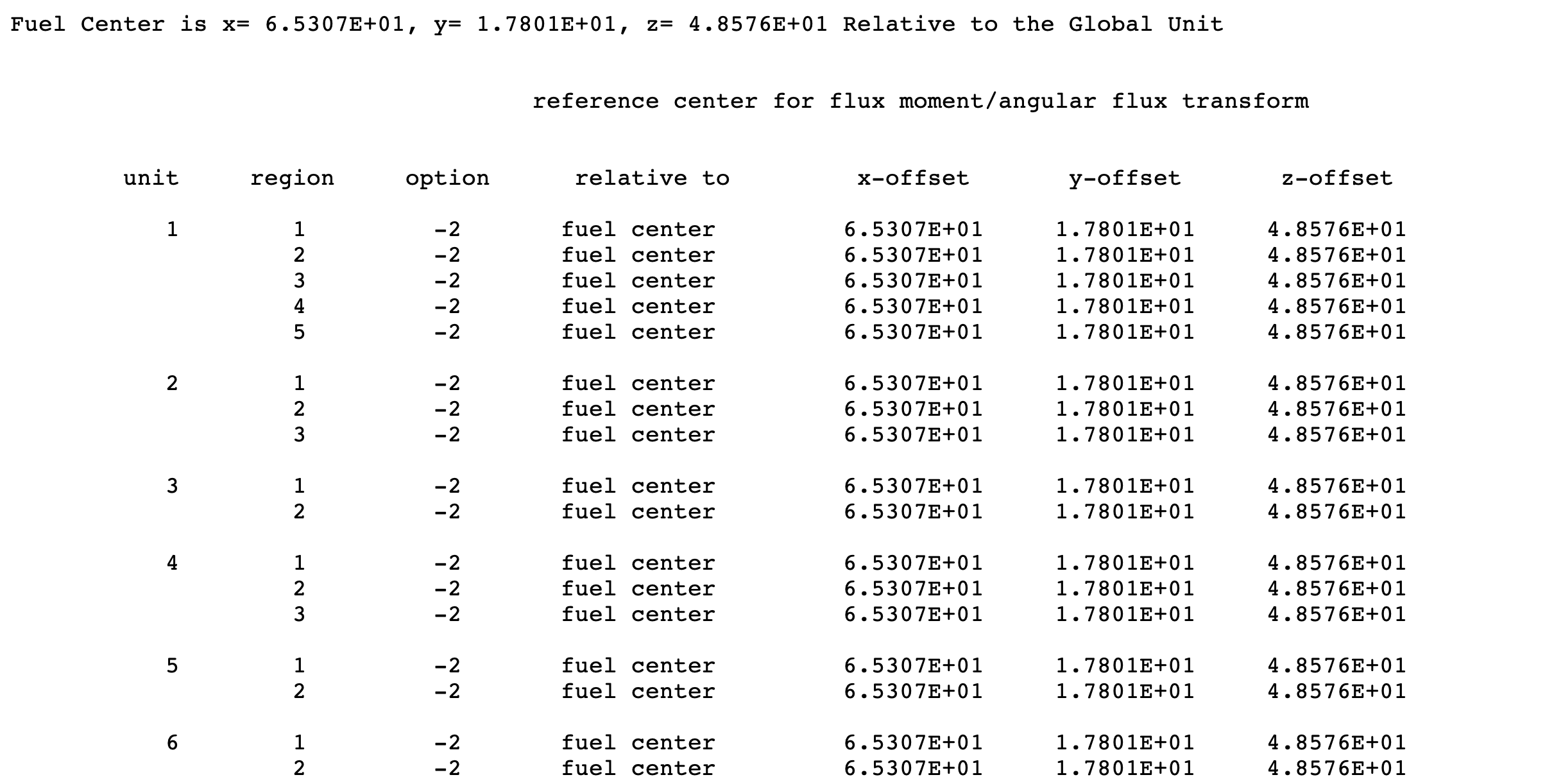
Fig. 8.1.135 Example fuel center and reference center edits.

8.1.5.25. Print starting points

This printout is optional and is used to verify the initial source starting points. This option is activated by specifying the parameter PSP=YES in start data block, and it is valid with all start types available. Examples of this information are given in Fig. 8.1.136.

The information pertinent to the initial source distribution is printed three lines at a time and appears under the designated headings. For example, the coordinates X, Y, and Z are printed on one line, the direction cosines U, V, and W are printed directly under them, and the global coordinates XGBL, YGBL, and ZGBL on the last line. The data printed for each source neutron include the following:

NEUTRON

is the ID number of the neutron.

X, Y, and Z

are the coordinates of the starting point relative to the coordinate system of the unit.

WT

is the starting weight (WT is always 1.0 for a neutron when it is started).

K

is the region number that contains the point X, Y, Z.

NOW

is the array number.

NBX, NBY, NBZ

are the coordinates of the unit within the array.

LL

is the unit number located at NBX, NBY, NBZ.

KR

is the mixture number present at the starting point.

KI

is the bias ID number or importance region at the starting point.

KCOR

is the region in the unit that contains the array where the neutron is located.

U, V, and W

are the direction cosines defining the direction the history is traveling.

IG

is the energy group.

K1

is the region number of the first region in unit LL.

K2

is the region number of the last region in unit LL.

IGEO

is an integer that defines the geometry shape of the region.

KCOL

is the region number in which the last collision occurred.

RANDOM NUMBER

is the current random number.

XGBL, YGBL, ZGBL

are the coordinates of the starting point relative to the coordinate system of the global unit.

UGBL, VGBL, WGBL

are the direction cosines defining the direction the history is traveling in the global coordinate system.

Note

When starting points are printed, many of the above named variables have not been initialized. For example, RANDOM NUMBER does not reflect the random number used to sample the starting point whose details are printed.

For starting, the variables of interest are X, Y, Z, NBX, NBY, NBZ, LL, XGBL, YGBL, and, ZGBL.

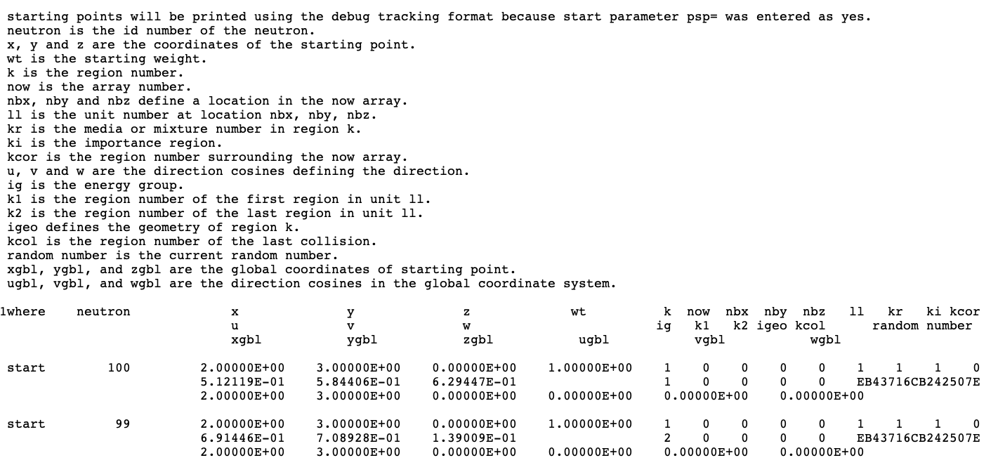
Fig. 8.1.136 Example of initial source points.

8.1.5.26. K-effectives by generation

At the completion of each generation, KENO prints the keff for that generation and associated information. An example of this printout is given in Fig. 8.1.137.

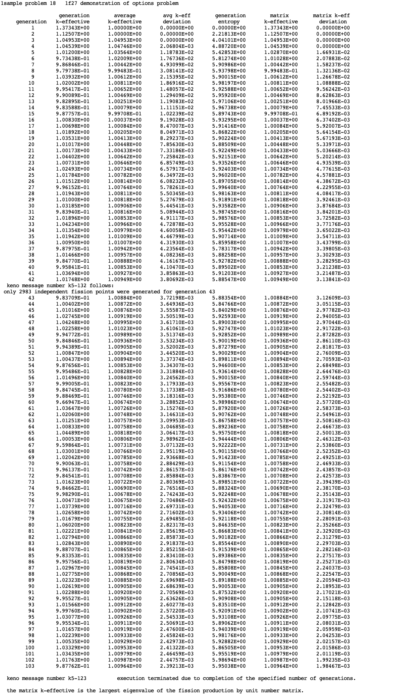
Fig. 8.1.137 Example of k-effectives and source entropy by generation.

The data printed include (1) the generation number, (2) the k-effective calculated for the generation, (3) the average value of k-effective through the current generation (excluding the nskip-1 generations), (4) the deviation associated with the average k-effective, (5) Shannon entropy for the generation, (6) the matrix k-effective for the generation, and (7) the deviation associated with the matrix k-effective. Column 5 is omitted if the user disabled source convergence diagnostics. The last two columns are filled with zeros if the user did not specify matrix k-effective calculations. The matrix k-effective is the largest eigenvalue of the fission production matrix. Matrix information can be calculated based on (1) position index, (2) unit number, (3) hole number, and (4) array number. The matrix k-effective printed in the sixth column is based on this order. If the matrix k-effective is calculated by position index, it is the one printed in the sixth column. The matrix k-effective by unit number is given second preference, followed by hole number and then array number.

After the last generation, a message is printed to indicate why execution was terminated. If matrix k-effectives were calculated, this is followed by a message stating the method used to determine the matrix k-effective.

The user should examine this portion of the printed results to ensure that the two methods of calculating k-effective are in acceptable agreement and to verify that the average value of k-effective has become relatively stable. If the k-effectives appear to be oscillating or drifting significantly, then the user should consider rerunning the problem with a larger number of histories per generation.

If a problem is restarted, then the generation numbers and k-effectives are printed and the words FROM RESTART UNIT are printed in the elapsed time column. All other columns are blank. When the generation at which the problem is to be restarted is reached, the print reverts to the normal format as shown in Fig. 8.1.137.

8.1.5.27. Problem characterization edit

The problem characterization edit follows the k-effective by generation edit. The title is printed at the top of the page, followed by the lifetime and the generation time and their associated deviations. The lifetime is the average lifespan of a neutron (in seconds) from the time it is born until it is absorbed or leaks from the system. The generation time is the average time (in seconds) between successive neutron generations. If NUB=YES is specified in the parameter data, (Sect. 8.1.3.3) the average number of neutrons per fission, NU BAR, and its associated deviation are printed and the AVERAGE FISSION GROUP (the average energy group at which fission occurs) and its associated deviation are printed. Then the ENERGY(EV) OF THE AVERAGE LETHARGY OF NEUTRONS CAUSING FISSION and its associated deviation are printed, followed by the system mean free path. If SMU=YES is specified in the parameter data, the average self-multiplication of a unit and its associated deviation is printed. This self-multiplication results from fissions caused by neutrons born in the unit. Fissions caused by neutrons that exit the unit and return are not included. The problem characterization edit is shown in Fig. 8.1.138.

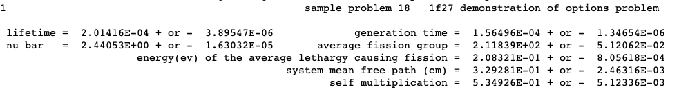
Fig. 8.1.138 Example problem characterization edit.

8.1.5.28. Final k-effective edit

The final k-effective edit prints the average k-effective and its associated deviation and the limits of k-effective for the 67, 95, and 99% confidence intervals. The number of histories used in calculating the average k-effective is also printed. This is done skipping various numbers of generations. The user should carefully examine the final k-effective edit to determine if the average k-effective is relatively stable. If a noticeable drift is apparent as the number of initial generations skipped increases, it may indicate a problem in converging the source. If this appears to be the case, the problem should be rerun with a better initial source distribution and should be run for a sufficient number of generations that the average k-effective becomes stable. The final k-effective edit is printed as shown in Fig. 8.1.139.

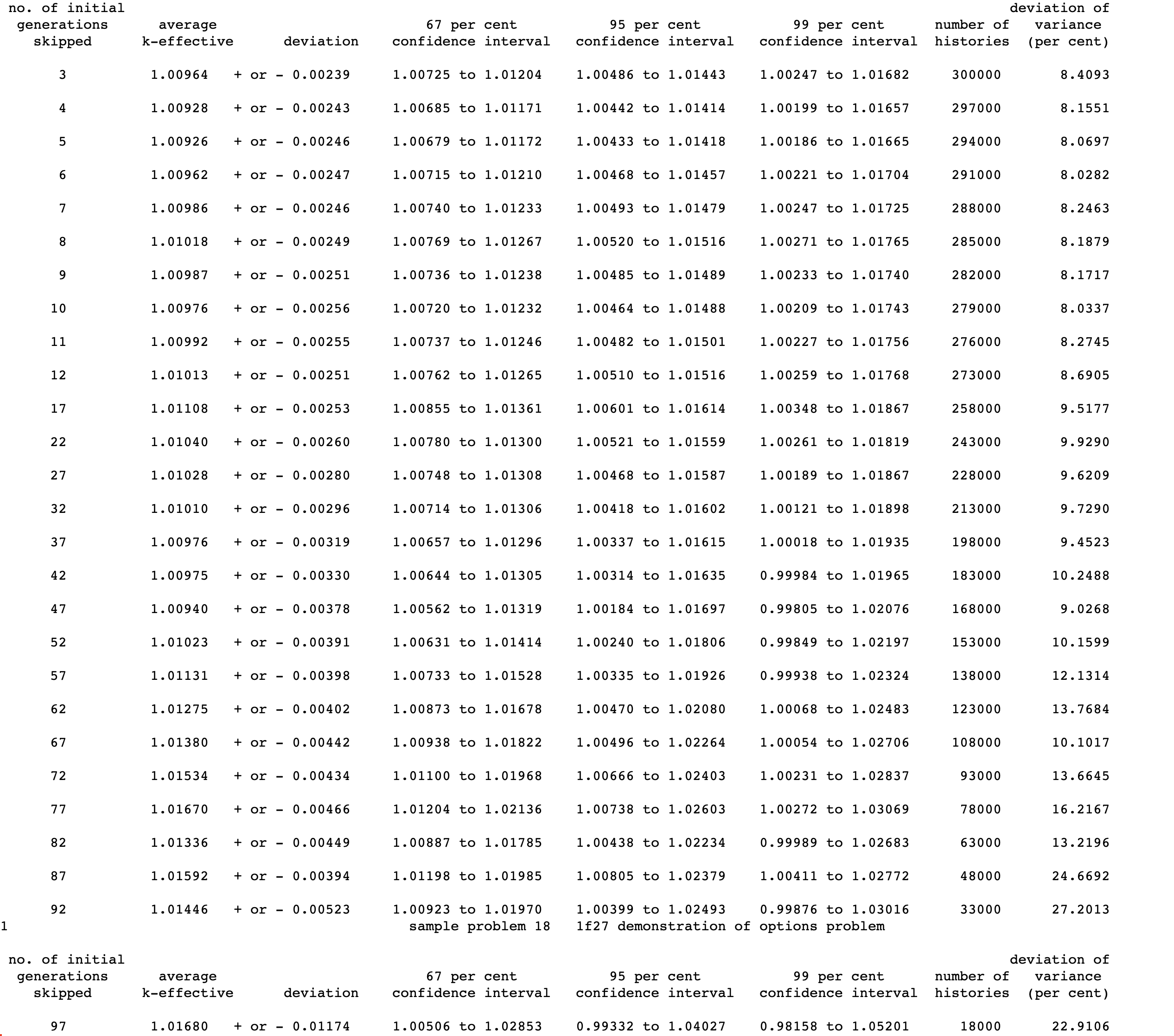
Fig. 8.1.139 Example of the final k-effective edit.

8.1.5.29. Plot of average k-effective by generation run

This plot consists of average k-effectives plotted versus the number of generations run. The limits of one standard deviation are plotted on either side of each average k-effective. These average k-effectives are not necessarily the same as the average k-effectives described in Sect. 8.1.5.26. The code omits the k-effectives of the first nskip generations when the average k-effectives for this plot are calculated. Although the k-effective of the nskip generation is summed into the average k-effective, it is not plotted because standard deviations cannot be calculated for a single point. Thus, if nskip is 3 (i.e., the first three generations are skipped), the first value plotted is the average k-effective corresponding to the fifth generation. The dotted line represents the value of the average k-effective corresponding to the smallest deviation when the average k-effective and its deviation are computed for each generation over the range of nskip through the total number of generations.

Fig. 8.1.140 is an example of this type of plot in the text output. The primary use for this plot is to determine if the problem has source convergence difficulties.

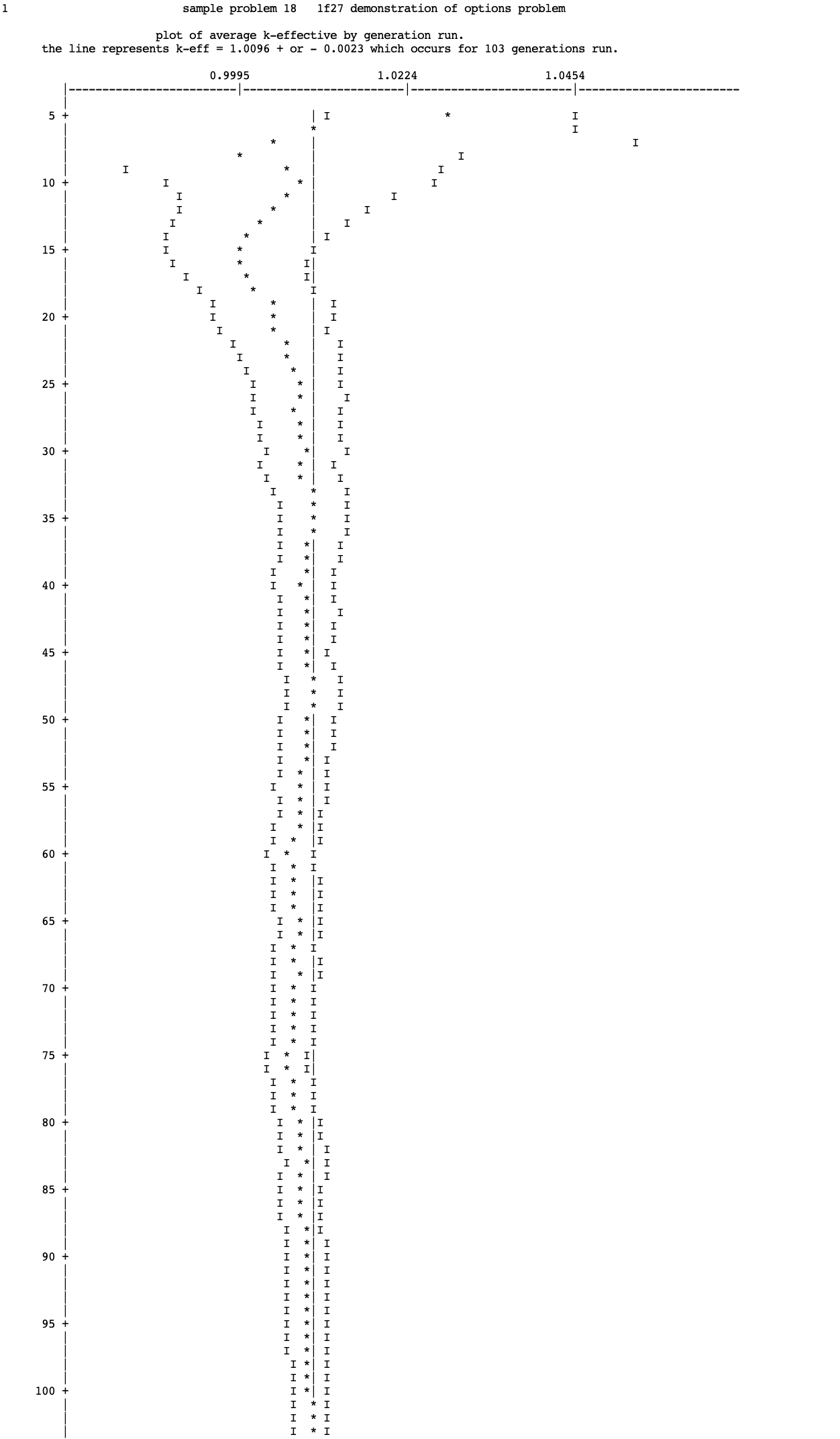
Fig. 8.1.140 Sample plot of average k-effective by generation run.

8.1.5.30. Plot of average k-effective by generations skipped

This plot illustrates the average k-effective versus the number of generations skipped as shown in Fig. 8.1.141. The limits of one standard deviation are plotted on either side of the average k-effective. The dotted line represents the value of the average k-effective corresponding to the smallest deviation when the average k-effective and its deviation are computed for the number of generations skipped over the range of nskip+1 through ²/₃ the total number of generations calculated. The plot is essentially a plot of the data described in Sect. 8.1.5.28. It is useful for determining if source convergence has been achieved.

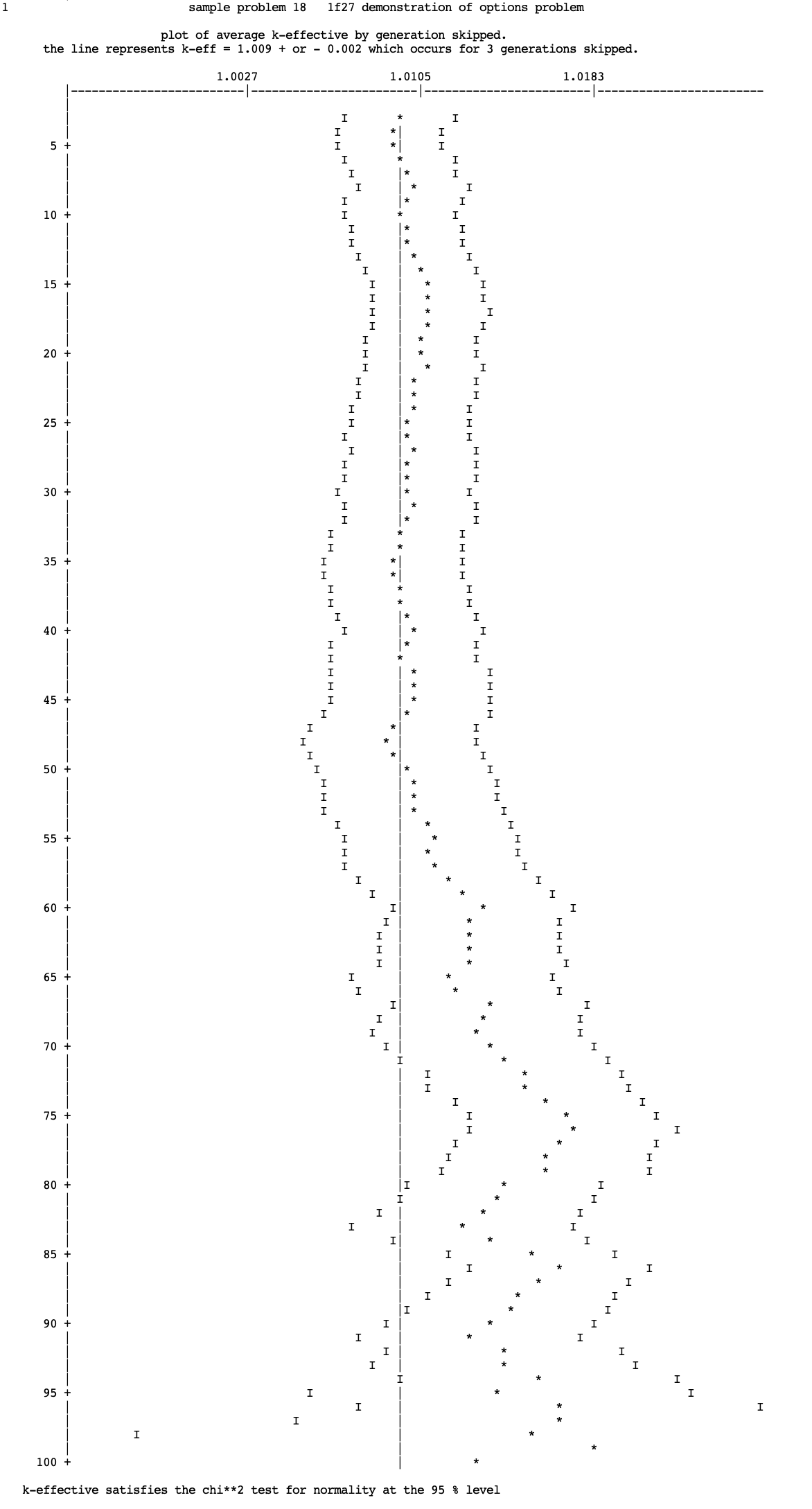
Fig. 8.1.141 Sample plot of average k-effective by generations skipped.

8.1.5.31. Final edit of fissions, absorptions, and leakage

The final edit of fissions, absorptions, and leakage follows the final k-effective edit and includes the fission fraction for each group and the fission production, absorptions, and leakage, each with its associated percent deviation. Examples of the final edits of fissions, absorptions, and leakage are shown in Fig. 8.1.142-Fig. 8.1.144.

If FAR=NO is specified, region-dependent fissions and absorptions are not printed. Fig. 8.1.142 demonstrates the printout if FAR=NO.

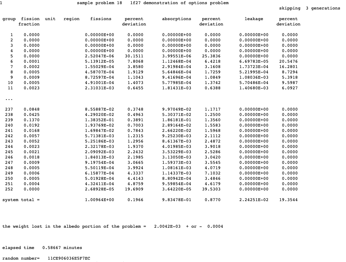
Fig. 8.1.142 Sample of the final edit of fissions, absorptions, and leakage with all region-dependent information suppressed (FAR=NO).

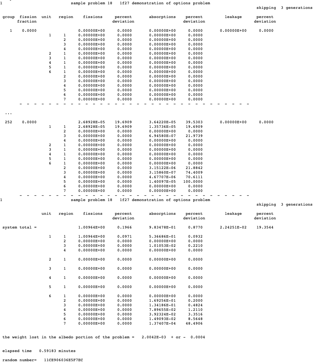
Fig. 8.1.143 Sample of the final edit of region-dependent fissions, absorptions, and leakage and the region-dependent totals (FAR=YES GAS=YES).

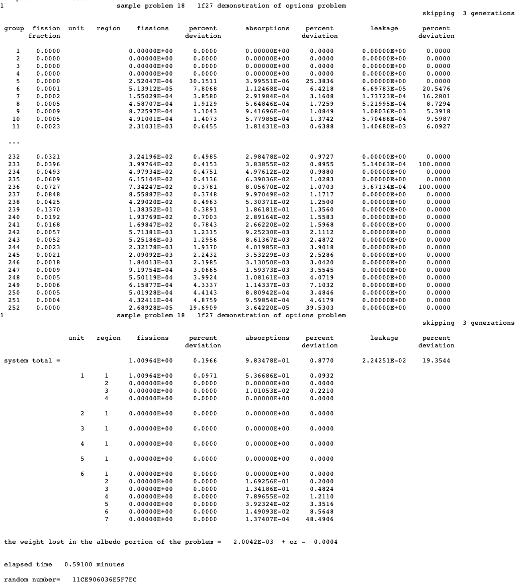
Fig. 8.1.144 Sample of the final edit of fissions, absorptions, and leakage and the region-dependent totals with print by region suppressed (FAR=YES GAS=NO).

If FAR=YES is specified in the parameter data, the fissions and absorptions for each geometry region used in the problem are calculated for each energy group. Leakage is not collected by geometry region, but rather it represents the leakage from the system. GROUP is the energy group number; FISSION FRACTION is the fraction of the fissions that occur in that energy group. The percent deviation for the fission fraction is the same as that of the fissions in the same group. The heading UNIT refers to the unit, and REGION is the region number within the specified unit. The geometry regions are numbered sequentially within each unit, starting with 1. The sum of the fissions for every region for a given energy group is the total printed for that energy group. The same is true of absorptions. The fissions, absorptions, and leakages are given in units of per source neutron. The SYSTEM TOTAL is the sum over all the energy groups of the fissions, absorptions, and leakage. The associated percent deviation is printed for each.

The parameter GAS is used to control printing of fission productions and absorptions for each geometry region by energy group as shown in Fig. 8.1.143. GAS=YES causes this data to be printed, provided FAR=YES is also specified. GAS=NO turns off this print by group as shown in Fig. 8.1.144.

The sum of the leakage and absorptions printed for the system total should be close to 1. The fissions printed for the system total should be the same as the first k-effective printed in the final k-effective edit described in Sect. 8.1.5.28. If differential albedos are used, the leakage does not include the weight lost in the albedo reflection. A message stating the weight lost in the albedo is printed. This is the weight lost due to absorptions in the albedo reflector and leakage from the albedo reflector. No leakage is associated with faces having specular, mirror image, or periodic reflection. Thus there is no leakage associated with an infinite problem. The total elapsed time and final random number are printed at the end of this edit.

8.1.5.32. Matrix k-effective by position index

The matrix k-effective by unit location (also referred to as array position or position index) is calculated if MKP=YES is specified in the parameter data and a global array is present in the model. It is the largest eigenvalue of the fission production matrix collected by position index. Sect. 8.1.4.13 provides a complete discussion of matrix k-effective. The POSITION INDEX is a number referencing a position in a 3-D lattice. POSITION is the X, Y, and Z location within the lattice. UNIT is the unit located at the specified location in the lattice. Thus, in Fig. 8.1.148 , UNIT 1 is located at the lower left-hand front corner of the array or 3-D lattice representing the problem (X=1, Y=1, Z=1) and the corresponding POSITION INDEX is 1. POSITION INDEX 8 is the top right-hand back corner of the lattice, POSITION X=2, Y=2, Z=2 and the unit located at that position is UNIT 8. An example of the matrix k-effective by position is given in Fig. 8.1.145 . The text output is contained within two rows of asterisks to draw attention to it.

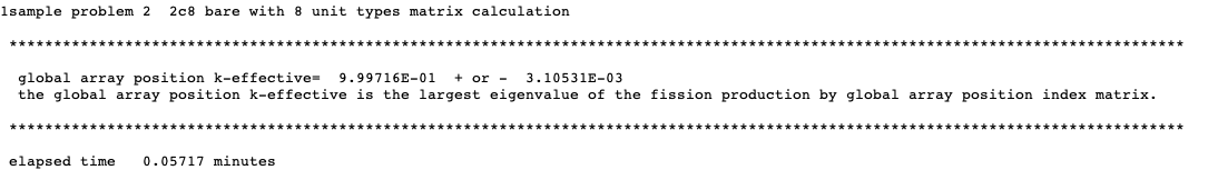
Fig. 8.1.145 Example of matrix k-effective by position index.

8.1.5.33. Fission production by position index matrix

To obtain fission production by position information, the user must specify MKP=YES and FMP=YES in the parameter data. The number of entries in the fission production matrix by position index is the square of the array size. Thus for a 2 \(\times\) 2 \(\times\) 2 array there are 64 entries, and for a 4 \(\times\) 4 \(\times\) 4 array there are 4,096 entries in the fission production matrix by position index. An example of the fission production matrix by position index for a 2 \(\times\) 2 \(\times\) 2 array is shown in Fig. 8.1.146.

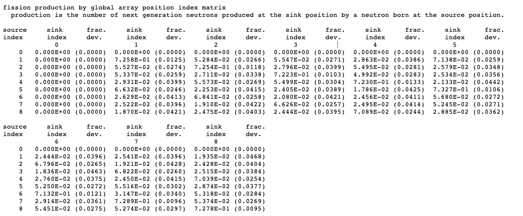
Fig. 8.1.146 Sample fission production matrix by position index.

For each position index in the array, the number of next-generation neutrons produced at position index J per neutron born at position index I is determined. The fission production matrix by position index is used to determine the matrix k-effective, cofactor k-effective and source vector by position index.

8.1.5.34. Source vector by position index

Source vector by position index information is printed if MKP=YES is specified in the parameter data. The source vector by position index is the eigenvector of the fission production matrix by position index and should sum to 1.0. It represents the fission source for the specified locations in the 3-D lattice representing the physical problem being analyzed. Position zero contains all material outside the global array. An example of the source vector by position index is shown in Fig. 8.1.147. The average self-multiplication by array position is the overall average of the self-multiplication of all units used in the problem.

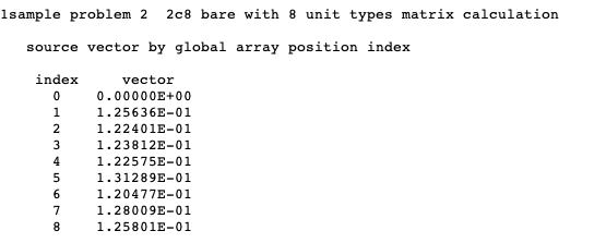
Fig. 8.1.147 Example of source vector by position index.

8.1.5.35. Cofactor k-effective by position index

The cofactor k-effective by position index edit is printed if MKP=YES is specified in the parameter data. This means that the fission production matrix is collected by position index. Calculating and printing cofactor k-effectives by position index can be avoided by specifying CKP=NO in the parameter data. An example of the cofactor k-effective by position index is shown in Fig. 8.1.148. See KENO Sect. 8.1.8.3 for a description of the problem used for the example.

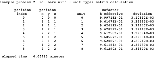
Fig. 8.1.148 Example of cofactor k-effective by position index.

The cofactor k-effective for a given position index is the largest eigenvalue of the fission production matrix collected by position index, reduced by the row and column associated with that position index. Thus the cofactor k-effective is the value of k-effective for the system calculated without the fission source of the unit located at the specified position index.

8.1.5.36. Matrix k-effective by unit number

The matrix k-effective by unit number (unit k-effective) is the largest eigenvalue of the fission production by unit matrix. It is calculated only if MKU=YES is specified in the parameter data. An example of the matrix k-effective by unit is given in Fig. 8.1.149.

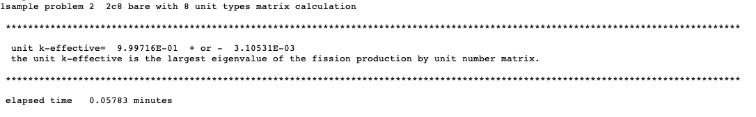
Fig. 8.1.149 Example of matrix k-effective by unit number.

8.1.5.37. Fission production by unit number matrix

The fission production by unit number matrix is computed and printed if MKU=YES and FMU=YES are specified in the parameter data. Thus, for each unit in the array, the number of next-generation neutrons produced in Unit J per neutron born in Unit I is determined. This is the fission production matrix by unit, and it is used to determine the matrix k-effective by unit, the cofactor k-effective by unit, and the source vector by unit. An example of the fission production matrix by unit is shown in Fig. 8.1.150 for text output.

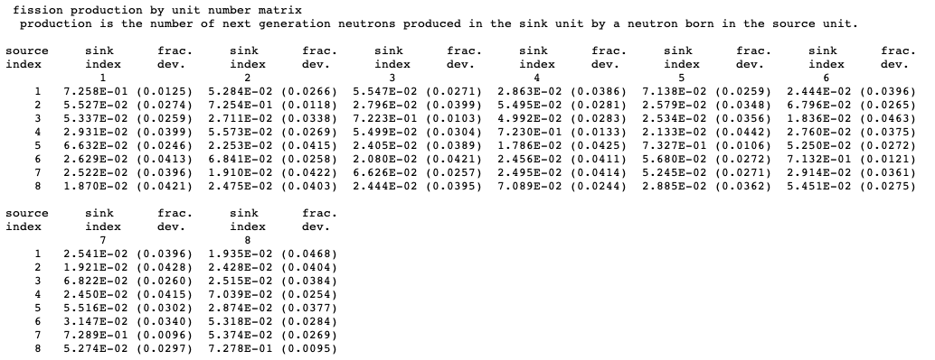
Fig. 8.1.150 An example of the fission probability matrix by unit.

8.1.5.38. Source vector by unit number

The source vector by unit is the eigenvector of the fission production matrix by unit and is printed if MKU=YES is specified in the parameter data. It represents the fission source for the units used in the problem. The components of the source vector should sum to 1.0. An example of the source vector by unit is given in Fig. 8.1.151. The average self-multiplication by unit is printed following the source vector. This value of self-multiplication includes those histories born in the unit which cause fissions in the same unit regardless of whether or not it exited and then returned. Therefore, this value will not agree with the value printed for the self-multiplication of the unit as described in Sect. Sect. 8.1.5.34 if the problem uses multiple units, if the system is reflected, or if a differential albedo is used in the problem.

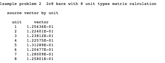
Fig. 8.1.151 Example of the source vector by unit.

8.1.5.39. Cofactor k-effective by unit number

The cofactor k-effective for a given unit is the k-effective of the system calculated without the fission source of that unit. Cofactor k-effectives are printed if MKU=YES is specified in the parameter data. Calculating and printing cofactor k-effectives by unit can be avoided by specifying CKU=NO in the parameter data. This step is accomplished by determining the eigenvalue of the fission production matrix by unit after it has been reduced by the row and column associated with that unit. An example of the cofactor k-effective by unit is given in Fig. 8.1.152.

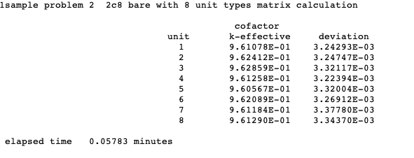
Fig. 8.1.152 Example of cofactor k-effective by unit number.

8.1.5.40. Matrix k-effective by hole number

The matrix k-effective by hole number is the largest eigenvalue of the fission production matrix collected by hole number and is calculated if MKH=YES was specified in the parameter data. An example of the matrix k-effective by hole number is given in Fig. 8.1.153.

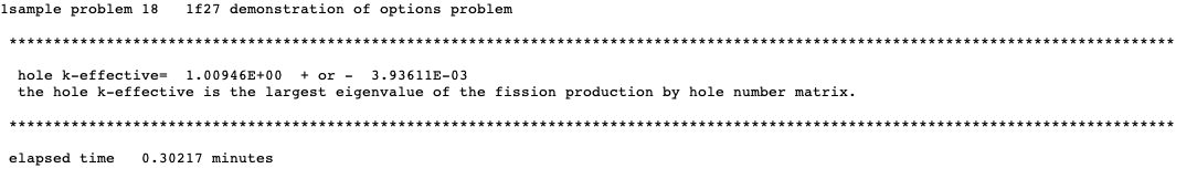
Fig. 8.1.153 Example of matrix k-effective by hole number.

8.1.5.41. Fission production by hole number matrix

This is the fission production matrix collected by hole number. It is printed only if MKH=YES and FMH=YES were specified in the parameter data. An example of this fission production matrix is given in Fig. 8.1.154. This matrix indicates the number of next generation neutrons produced in HOLE number J by a neutron born in HOLE number I.

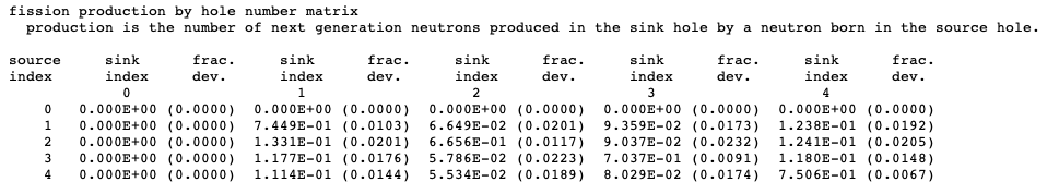
Fig. 8.1.154 Example of fission production matrix by hole.

8.1.5.42. Source vector by hole number

The source vector by hole is the eigenvalue of the fission production matrix by hole number and is printed if MKH=YES is specified in the parameter data. The source vector should sum to 1.0. An example of the source vector by hole is shown in Fig. 8.1.155. The average self-multiplication by hole is the overall average of the self-multiplication of all the holes in the problem.

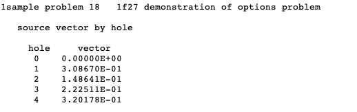
Fig. 8.1.155 Example of source vector by hole number.

8.1.5.43. Cofactor k-effective by hole number

The cofactor k-effective for a given hole is the k-effective of the system calculated without the fission source of that hole and is calculated if CKH=YES is entered in the parameter data. These values are computed by determining the eigenvalue of the fission production matrix by hole after it has been reduced by the row and column associated with that hole. An example of the cofactor k-effective by hole number is given in Fig. 8.1.156.

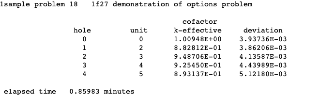
Fig. 8.1.156 Example of cofactor k-effective by hole number.

8.1.5.44. Matrix k-effective by array number

The matrix k-effective by array number is the largest eigenvalue of the fission production matrix collected by array number and is calculated if MKA=YES is entered in the parameter data. An example is given in Fig. 8.1.157 . The number of next generation neutrons produced in array number J by a neutron born in array number I is given in this fission production matrix.

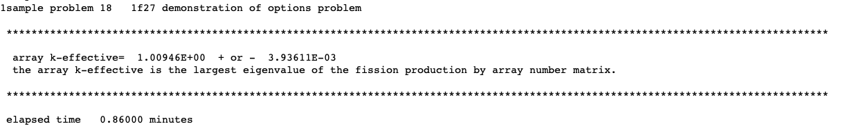
Fig. 8.1.157 Example of matrix k-effective by array number.

8.1.5.45. Fission production by array number matrix

The fission production matrix collected by array number is shown in Fig. 8.1.158 . It is printed only if MKA=YES and FMA=YES are specified in the parameter data.

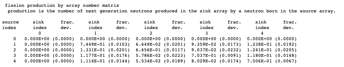
Fig. 8.1.158 An example of the fission production matrix by array number.

8.1.5.46. Source vector by array number

The source vector by array number is the eigenvector of the fission production matrix by array number and is printed if MKA=YES is specified in the parameter data. The source vector should sum to 1.0. An example of the source vector by array number is shown in Fig. 8.1.159. The average self-multiplication by array number is the overall self-multiplication of all the arrays in the problem.

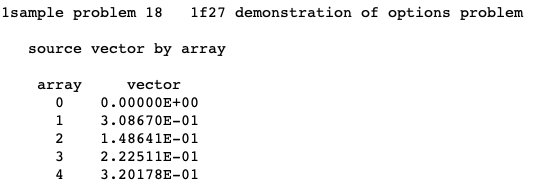
Fig. 8.1.159 Example of source vector by array number.

8.1.5.47. Cofactor k-effective by array number

The cofactor k-effective by array number is the k-effective of the system calculated without the fission source of that array and is calculated if CKA=YES is entered in the parameter data. This is achieved by determining the eigenvector of the fission production matrix by array after reducing it by the row and column associated with the specified array. Fig. 8.1.160 is an example of the cofactor k-effective by array number.

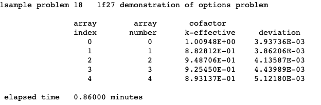
Fig. 8.1.160 Example of cofactor k-effective by array number.

8.1.5.48. Mesh tallies

The mesh tallies edit is optional. KENO prints the specification of each mesh tally defined by CDS=, FIS=, and GFX= parameters. A sample mesh tallies edit is given in Fig. 8.1.161. This edit does not print any details for both the mesh flux tally activated by MFX= and the \(F^{*}(r)\) mesh tally controlled by CGD= parameters.

At the top of this output edit, the number of tallies computed for the given problem is printed. Then, a summary section including the tally response, spatial and energy grid identifiers, approximate memory required to compute and write this tally data, and tally 3dmap output filename is provided. The grid identifier points to the spatial mesh grid defined either with MSH= parameter or grid geometry data input block. Similarly, the energy identifier points to the DEFAULT energy boundaries (see Sect. 8.1.5.13). A summary of the energy and spatial grids is presented after this section. Details of both energy boundaries and grid definitions used for these mesh tallies can be seen in Sect. 8.1.5.13 and Sect. 8.1.5.19.

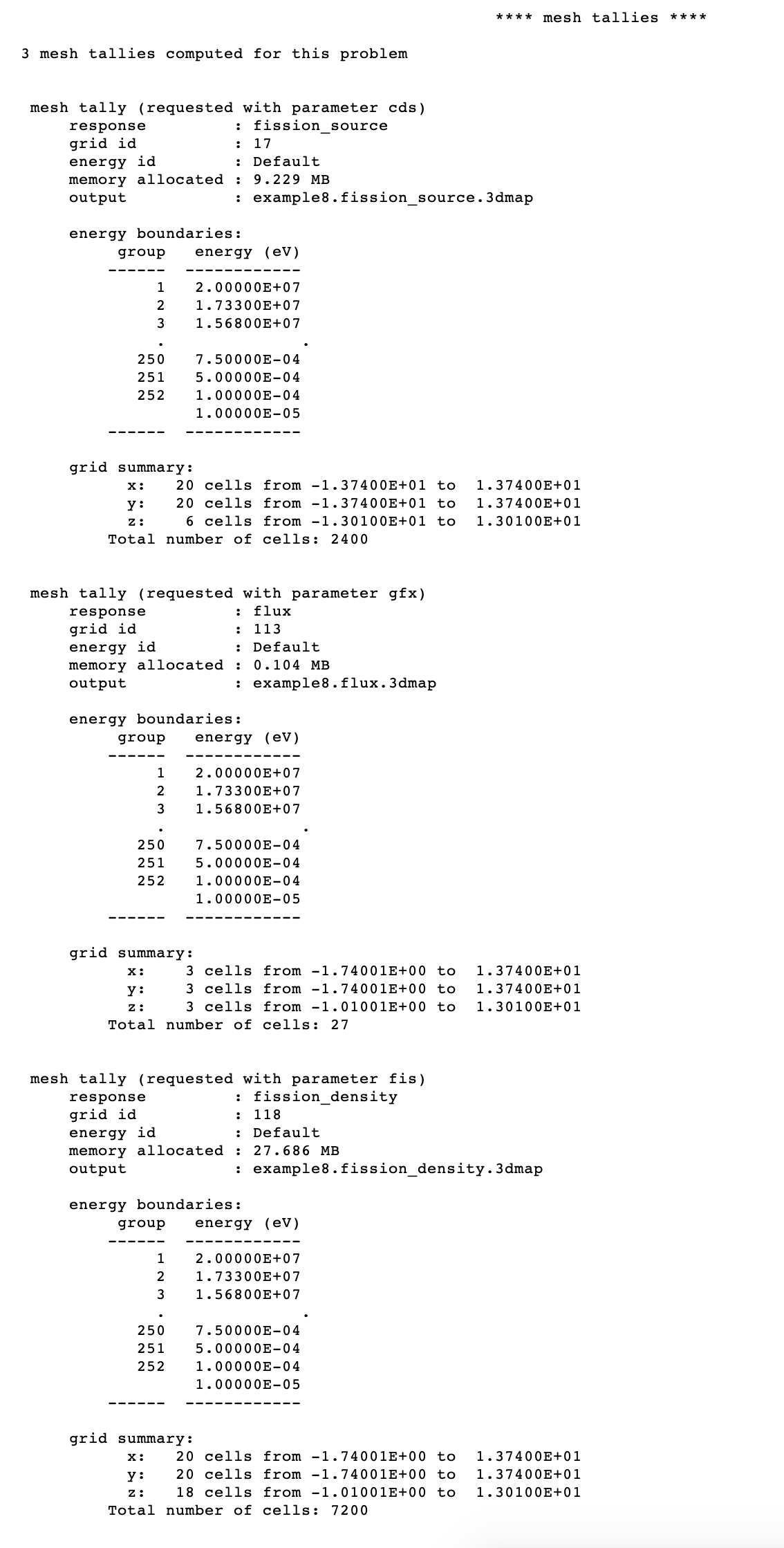
Fig. 8.1.161 Example of mesh tallies output edit.

Note

Tally results stored in 3dmap files can be visualized by Fulcrum mesh tally plotting capability. Similarly, they can be processed by using the utility tools provided by MAVRIC utilities.

8.1.5.49. Reaction tally

Reaction tally calculations are performed if the required data are specified in the reaction data block (Sect. 8.1.3.15). KENO prints a table in the output that summarizes the parameter specifications in reaction tally calculations. An example of the parameter table for the reaction tally calculations is shown in Fig. 8.1.162.

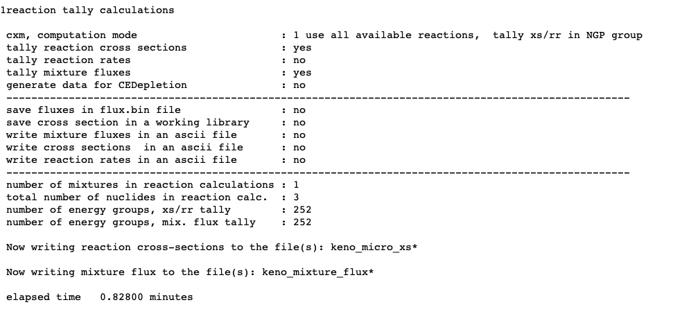
Fig. 8.1.162 Example of reaction tally summary table.

8.1.5.50. Source convergence diagnostics edit

KENO calculates the Shannon entropy of the fission source distribution at each generation and reports this in the problem output (Sect. 8.1.5.26). At the end of calculation, KENO performs three tests to check the fission source convergence and reports these test results in the output. (See Sect. 8.1.7.7 for the definition of these tests.) An example of the fission source convergence diagnostics is given in Fig. 8.1.163. The last entry in this output edit is the plot of Shannon entropy by generations run, and a sample Shannon entropy plot is shown in Fig. 8.1.164.

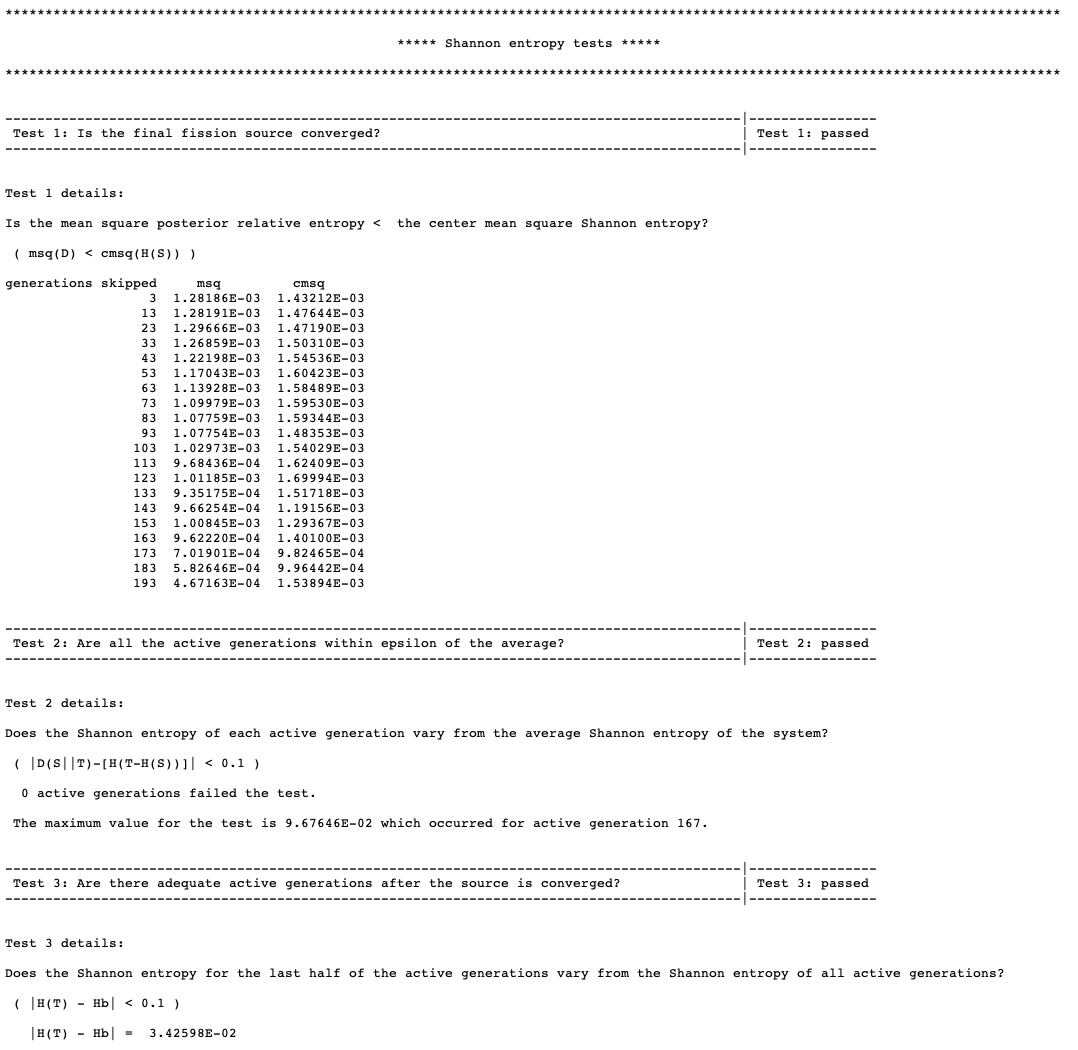
Fig. 8.1.163 Summary of fission source convergence diagnostics.

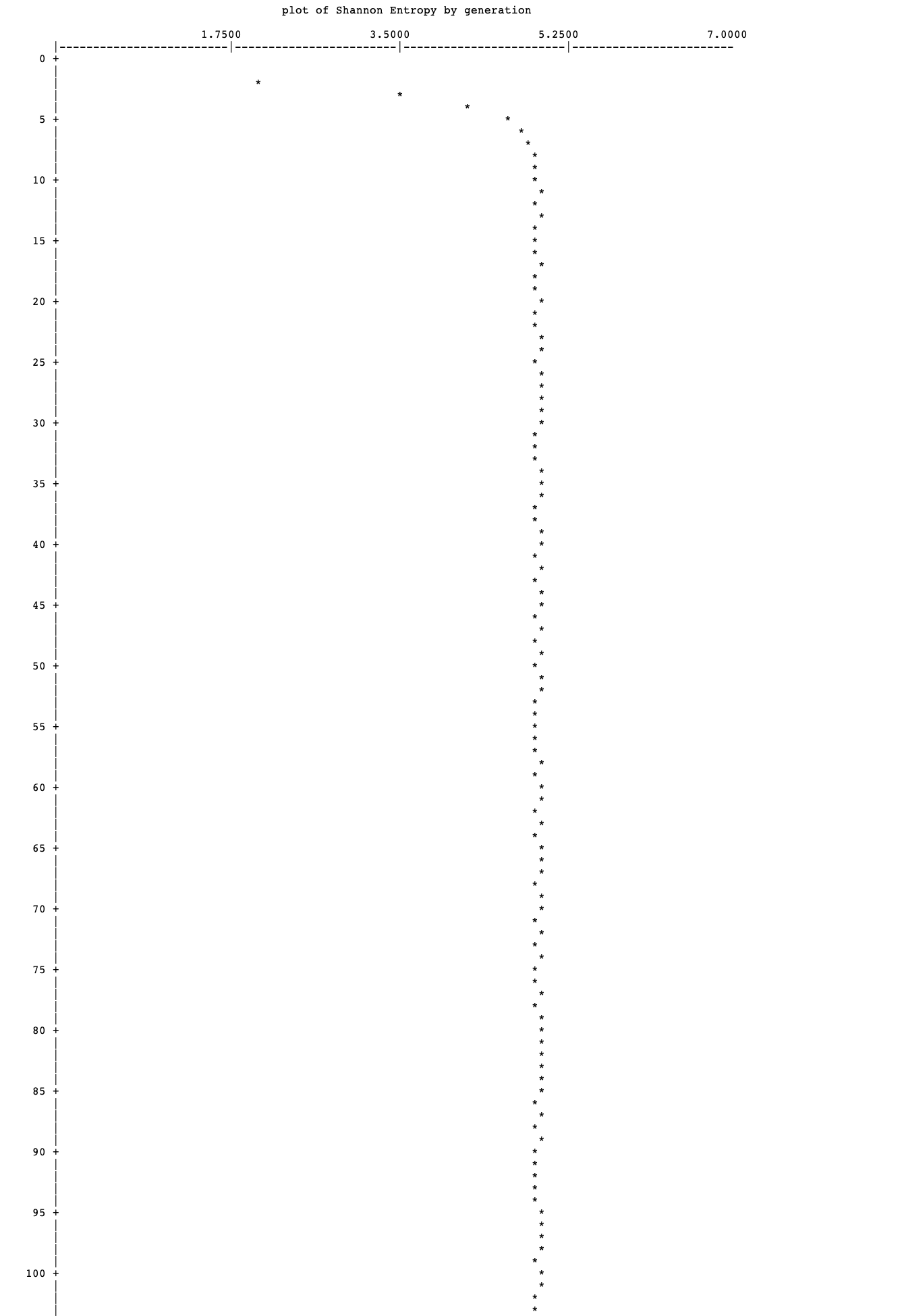
Fig. 8.1.164 A sample Shannon entropy plot.

8.1.5.51. Fission density edit

The fission density edit is optional. Subroutine KEDIT prints the neutron production density and the fission density for each geometry region if FDN=YES and NUB=YES is specified in the parameter data (these are the default values). If NUB=NO is specified, but FDN=YES, then only the production density will be given. An example of the fission density edit is shown in Fig. 8.1.165.

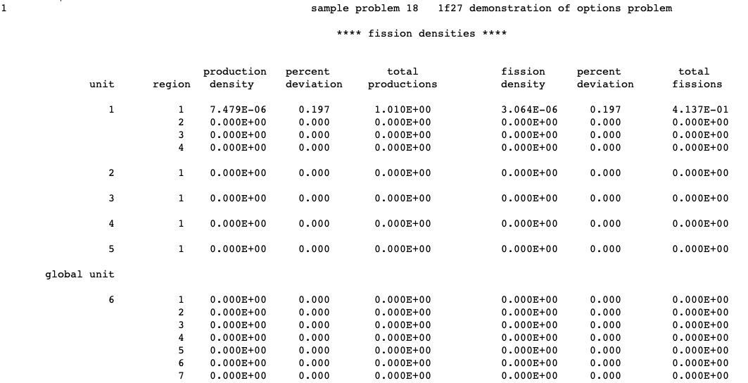
Fig. 8.1.165 Example of the fission density edit.

The UNIT is the unit number from the geometry data, the REGION is the region number relative to the unit, the PRODUCTION DENSITY is the neutrons produced per cm³ per source-neutron, and the FISSION DENSITY is the fissions per cm³ per source-neutron for that geometry region, the PERCENT DEVIATION is 100 times the fractional standard deviation associated with the production density and/or the fission density, the TOTAL PRODUCTIONS is the total number of neutrons produced per source neutron, and the TOTAL FISSIONS is the total number of fissions per source neutron in the geometry region.

8.1.5.52. Flux edit

Printing the region fluxes is optional; they are only printed if FLX=YES is specified in the parameter data. The fluxes are printed for each unit and each geometry region in the unit for every energy group. A sample of a flux edit is given in Fig. 8.1.166.

The title of the problem is printed at the top of the page. The heading FLUXES FOR UNIT____ indicates the geometry unit for which fluxes are being printed. The region numbers relative to the unit are identified by the heading REGION____. The geometry regions within each unit are numbered sequentially, beginning with 1. Then, the volume of each region is printed. Note that if the region volume is printed as -1.0, it indicates that either volume is not defined for this region, or that volume is not calculated, or it is calculated as 0.0. GROUP is the heading for the energy groups. The headings FLUX and PERCENT DEVIATION are printed for each geometry region in the unit. The flux and its associated percent deviation are printed for every energy group and every geometry region. The last entry printed for the flux edit is the TOTL which is the total flux integrated over all energy groups for each region. The flux is in units of neutrons/cm² /source neutron.

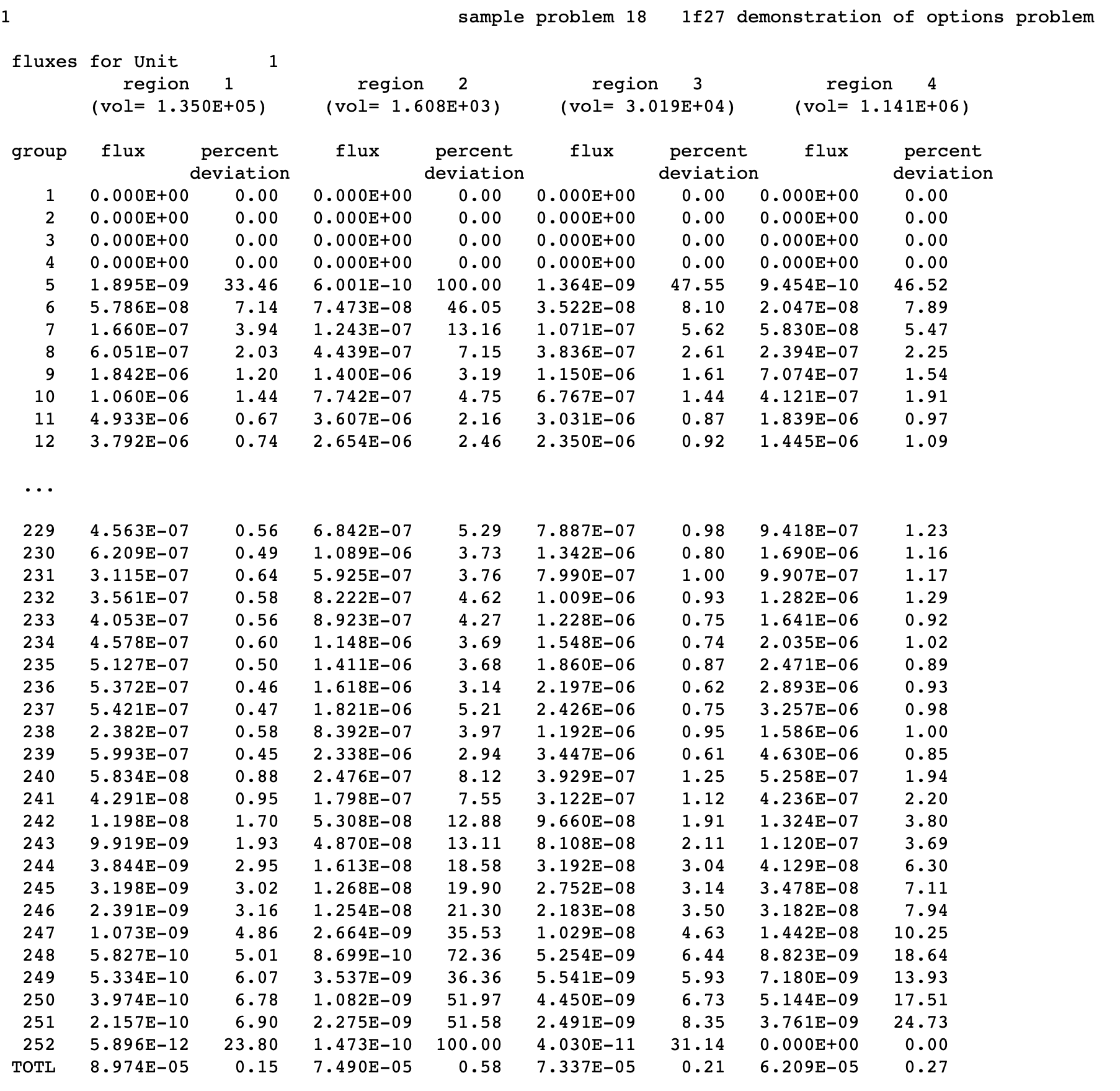
Fig. 8.1.166 An example of a flux edit.

8.1.5.53. Frequency distributions

A frequency distribution consists of a bar graph indicating the number of generations having k-effective in a specified interval. The intervals are determined by the code, based on the upper and lower limits of the k-effectives calculated for the generations. In this example, one asterisk is printed for each generation k-effective. Four frequency distributions are printed as shown in Fig. 8.1.167. These four plots are: (1) all active generations, (2) the last 3/4 of active generations, (3) the last half of active generations, and (4) the last quarter of active generations. Note that departures from normal distributions in these plots and radical shifts among them may be indications of source convergence issues in the calculation.

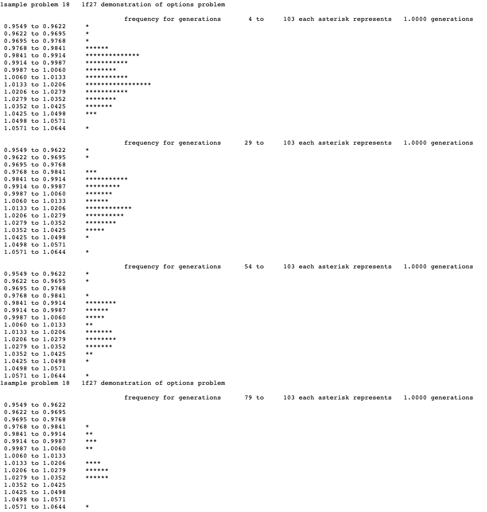
Fig. 8.1.167 An example of a frequency distribution.

8.1.5.54. Summary of parallel performance

KENO summarizes parallel performance in the output if parallel execution is requested by the user. The performance table, shown in Fig. 8.1.168, can be used to evaluate the code parallel performance with the given problem parameters. The quantities like speedup, parallel efficiency, and wall-clock time for each section (serial section, parallel section, and communication time among the processors) can be used to estimate resource requirement for similar problems to accomplish a faster execution.

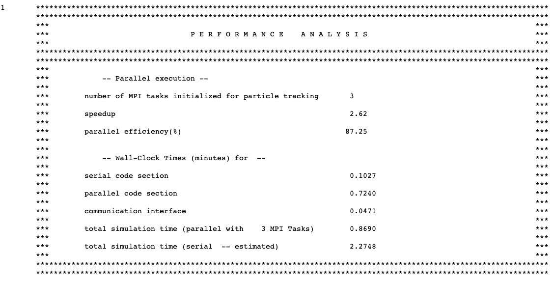
Fig. 8.1.168 Example of performance analysis table.

8.1.5.55. Final results table

The final results table contains a summary of the most important physics parameters of the system and the number of error and warning messages generated during execution. The table contains the best-estimate system k-effective with one standard deviation, the energy of the average lethargy of fission, the average system nu-bar, the average mean free path of a neutron throughout the system, the number of warning and error messages generated during code execution, and a final statement on the convergence of the \(\chi\)² test results. A summary of the Shannon entropy source convergence diagnostics is printed here. See the details of tests in Sect. 8.1.5.50 and Sect. 8.1.7.7. An example of this table is shown in Fig. 8.1.169. Also shown is the terminal edit of KENO, detailing the time required to traverse the “perilous path” through KENO.

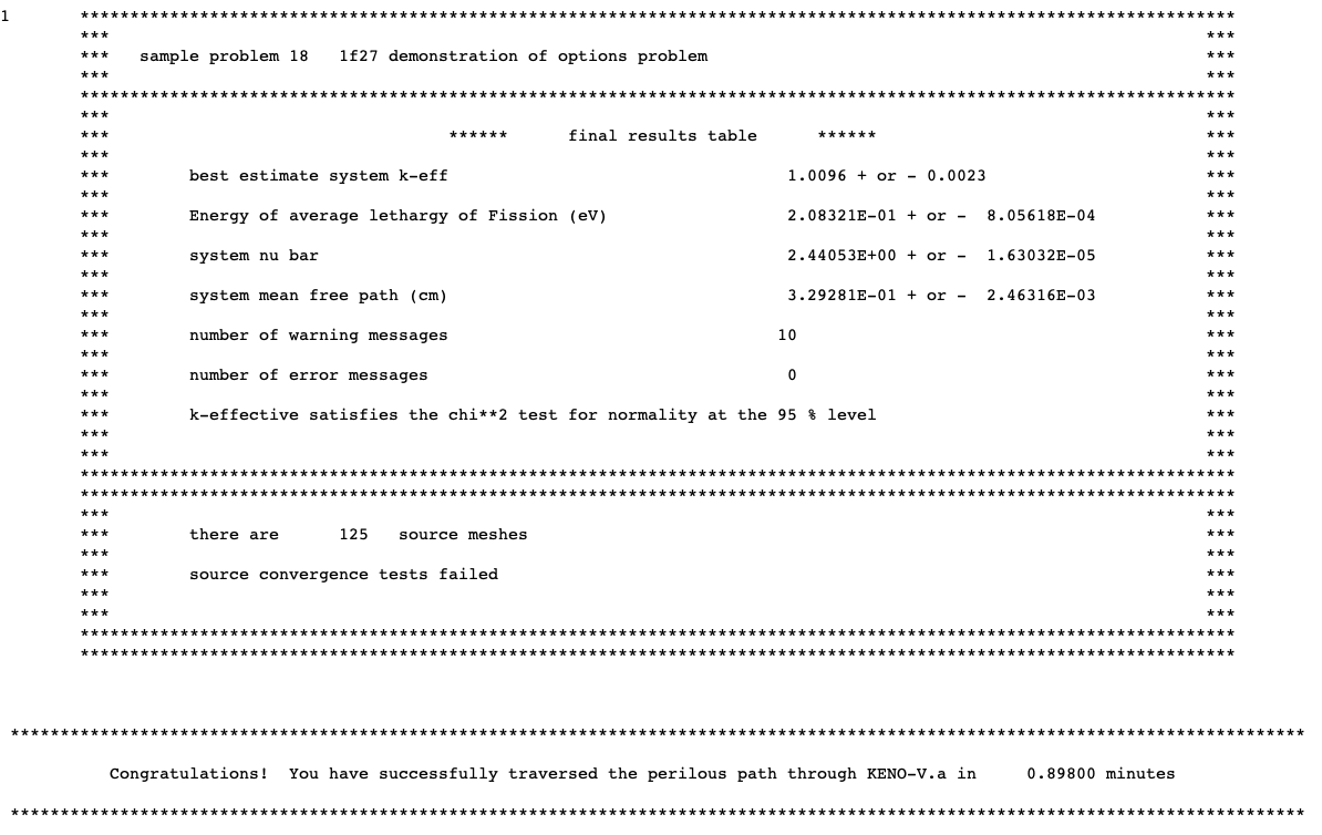
Fig. 8.1.169 An example of the final results table.

8.1.5.56. HTML output

The HTML-formatted output is no longer actively developed, and the output files created with it may therefore not include recently added capabilities or changes. For example, the fission rate mesh tally and some CE TSUNAMI edits are not included in the HTML output.

8.1.5.56.1. HTML output: Program verification information

The program verification information is the first page shown in the KENO HTML output, after selecting KENO from the SCALE HTML index page. This page can also be displayed by selecting the Program Verification Information link under the General Information submenu and is shown in Fig. 8.1.170.

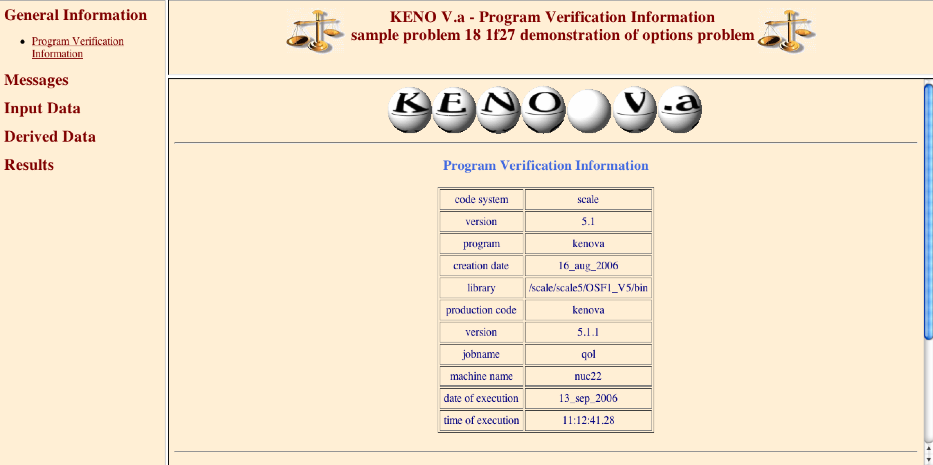
Fig. 8.1.170 Sample program verification information in HTML output.

8.1.5.56.2. HTML output: Messages

In the HTML output, all error and warning messages are consolidated into the Messages section of the output. Error Messages and Warning Messages links are available to the user as needed. An example edit with warning messages is shown in Fig. 8.1.171.

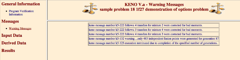
Fig. 8.1.171 Example messages edit in HTML output.

8.1.5.56.3. HTML output: Tables of parameter data

The first two tables generated by KENO HTML output list the numeric parameters and logical parameters that are used in the problem. The user should always verify that the parameter data block was input as desired. An example of numeric parameters table is shown in Fig. 8.1.172. An example of the logical parameters table is shown in Fig. 8.1.173. The HTML output is accessed with the Numeric Parameters and Logical Parameters links in the Input Data section.

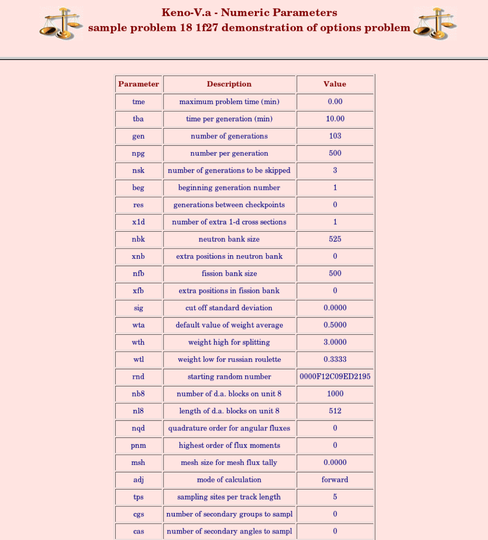
Fig. 8.1.172 Sample numeric parameters in HTML output.

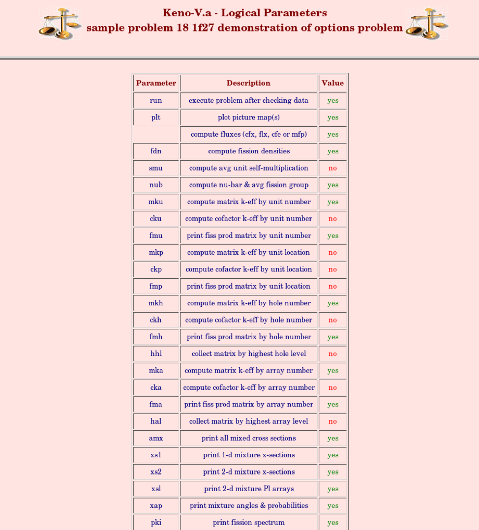
Fig. 8.1.173 Sample logical parameters in HTML output.

8.1.5.56.4. HTML output: Table of additional information

The fourth table of data printed by KENO contains additional information determined from the input data. An example of this table is shown in Fig. 8.1.174. The HTML output is accessed with the Additional Information link in the Input Data section.

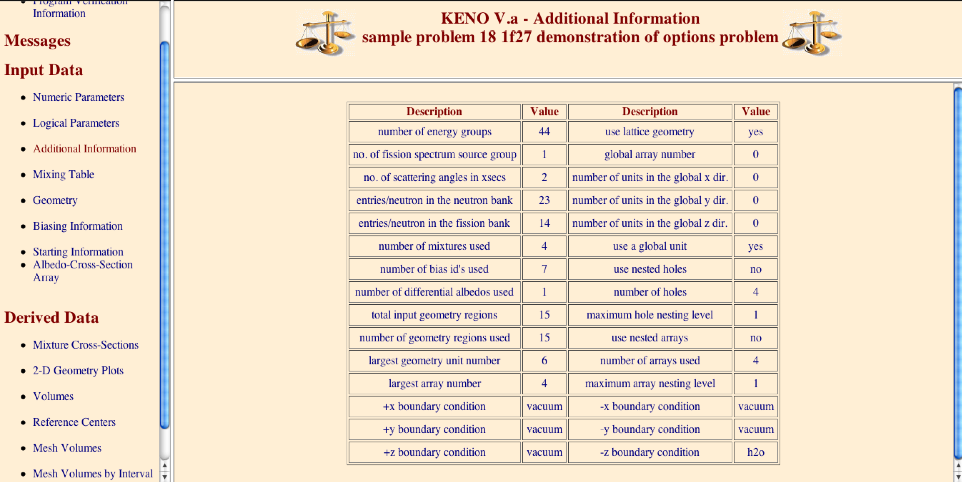
Fig. 8.1.174 Sample table of additional information in HTML output.

8.1.5.56.5. HTML output: Mixing table data

If LIB= is entered in the KENO parameter data and a mixing table data block is provided to KENO, then mixing table data will be printed. Sample mixing table data are shown in Fig. 8.1.175. In the HTML output, the mixing table data can be accessed with the Mixing Table link in the Input Data section.

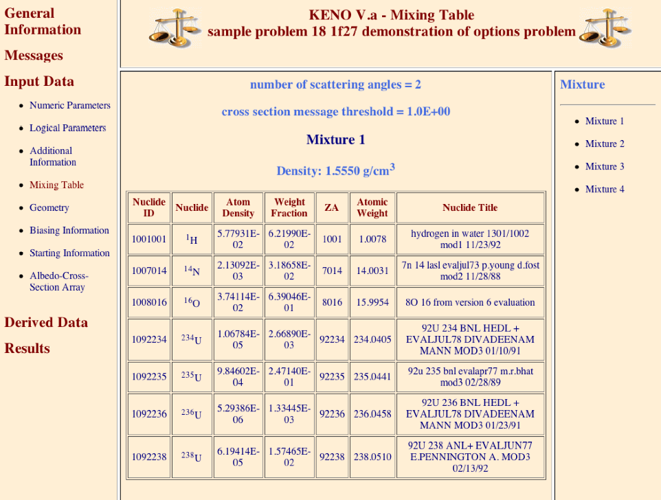
Fig. 8.1.175 Example of mixing table data in HTML output.

8.1.5.56.6. HTML output: 1D macroscopic cross sections

The decision to print the 1-D mixture cross sections is optional. They are printed only if XS1=YES is specified in the parameter data. The 1-D mixture cross sections for a mixture are shown in Fig. 8.1.176. The HTML output is accessed with the Mixture Cross Sections link in the Derived Data section. The top menu on the right side of the window is used to set the mixture displayed in the bottom menu on the right side of the window. The bottom menu contains hyperlinks to all available edits for mixture cross sections. The 1-D cross sections are accessed with the Neutron Cross Sections link in the bottom menu for the desired mixture.

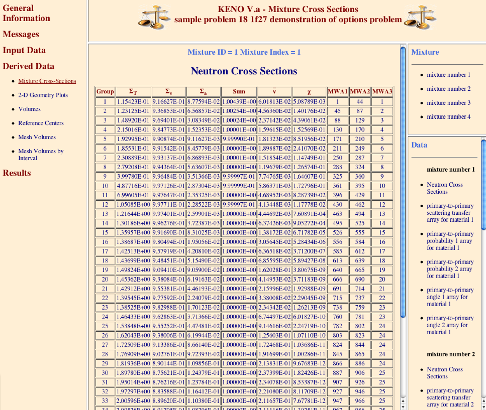
Fig. 8.1.176 Example 1-D macroscopic cross section in HTML output.

When the 1-D mixture cross sections are printed, the problem title is printed at the top of the page. The mixture ID, mixture index and mixture number are then printed. ID is the mixture number from the mixing table and mixture index is the index used to reference it and mixture number is its identifier. This step is followed by a heading to identify the different 1-D cross sections. GROUP is the energy group, sigt is the total cross section for the mixture, sigs is the nonabsorption probability, siga is the absorption probability, signu is the production probability, chi is the fission spectrum, mwa1 is the pointer for the first position of the cross sections for the energy group, mwa2 is the pointer for the last position of the cross sections for the energy group, and mwa3 contains the group for the transfer corresponding to the first position. SUM is the sum of the absorption probability and the nonabsorption probability. The nonabsorption probability and the production probability are not true probabilities in that they may be greater than 1. This is because the nonabsorption probability has the (n,2n) transfer array summed into the total transfer array twice, and the (n,3n) is summed three times, etc. The absorption probability is defined as the absorption cross section divided by the total cross section. The nonabsorption probability is the sum of the group-to-group transfers for this group divided by the total cross section. The production probability is defined as the fission production cross section divided by the total cross section \(\left(\nu \Sigma_{f} / \Sigma_{\mathrm{T}}\right)\).

8.1.5.56.7. HTML output: 2-D macroscopic cross sections

The decision to print the 2-D mixture cross sections is optional. An example of the 2-D mixture cross sections is given in Fig. 8.1.177. The HTML output is accessed with the Mixture Cross Sections link in the Derived Data section. The top menu on the right side of the window is used to set the mixture displayed in the bottom menu on the right side of the window. The bottom menu contains hyperlinks to all available edits for mixture cross sections. The 1-D macroscopic cross sections are accessed with the primary-to-primary scattering transfer array link in the bottom menu for the desired mixture.

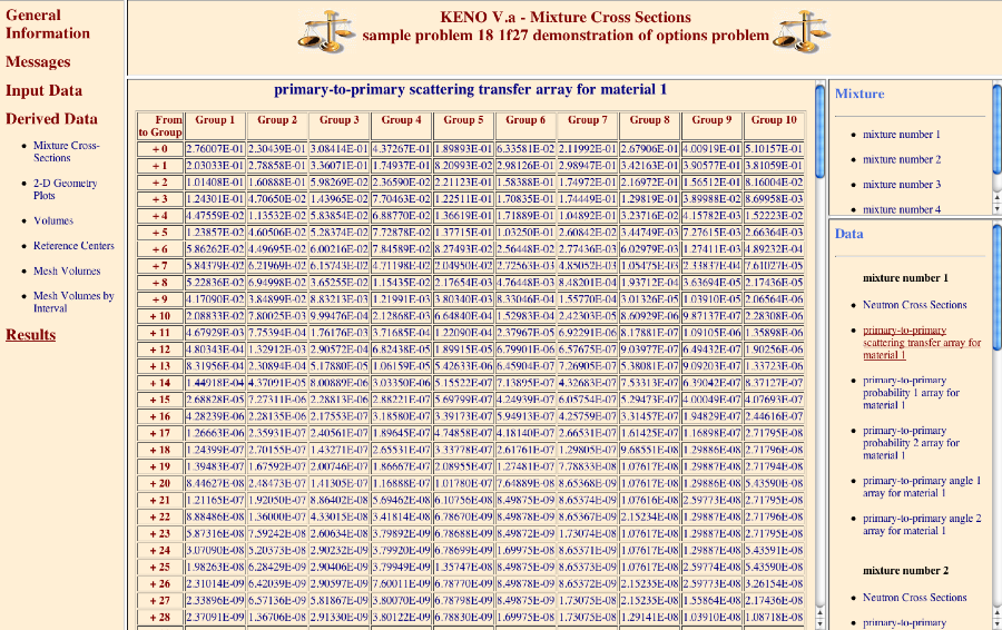
Fig. 8.1.177 Example of 2-D macroscopic cross sections in HTML output.

8.1.5.56.8. HTML output: Probabilities and angles

Printing the probabilities and angles is optional. The HTML output, Fig. 8.1.178, is accessed with the Mixture Cross Sections link in the Derived Data section. The top menu on the right side of the window is used to set the mixture displayed in the bottom menu on the right side of the window. The bottom menu contains hyperlinks to all available edits for mixture cross sections. The probabilities and angles edits, shown in Fig. 8.1.179, are accessed with the primary-to-primary probability link in the bottom menu for the desired mixture.

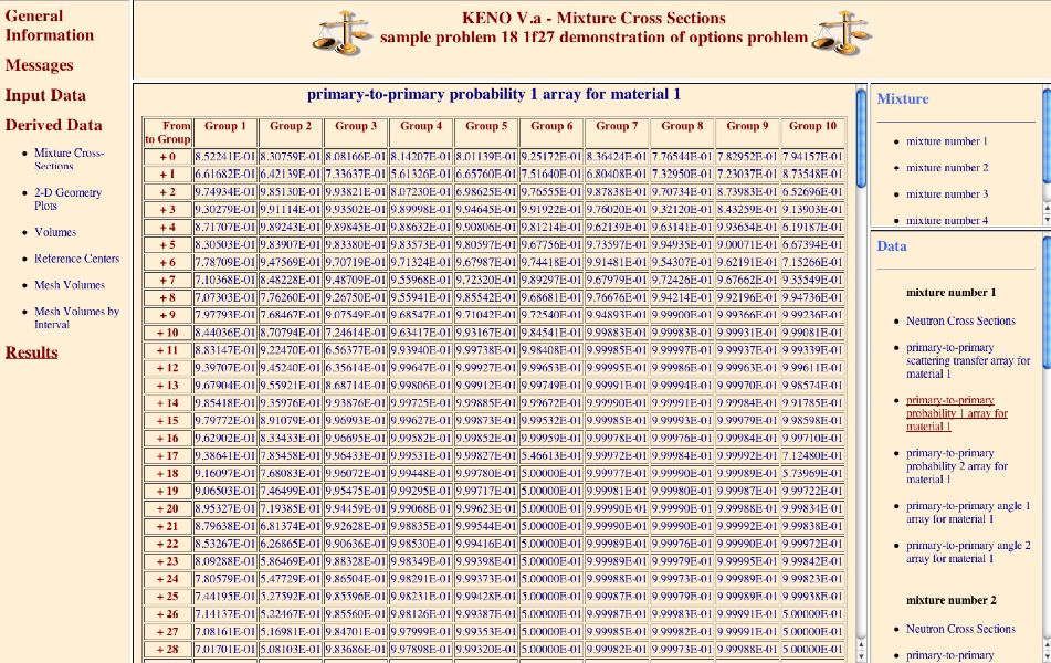
Fig. 8.1.178 Example of macroscopic probabilities in HTML output.

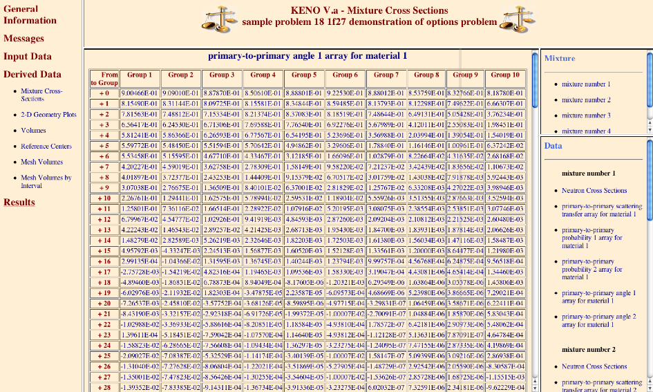
Fig. 8.1.179 Example of macroscopic angles in HTML output.

8.1.5.56.9. HTML output: Geometry data

The KENO V.a HTML version of the geometry region printout is shown in Fig. 8.1.180. The HTML edits of geometry are accessed with the Geometry link in the Input Data section.

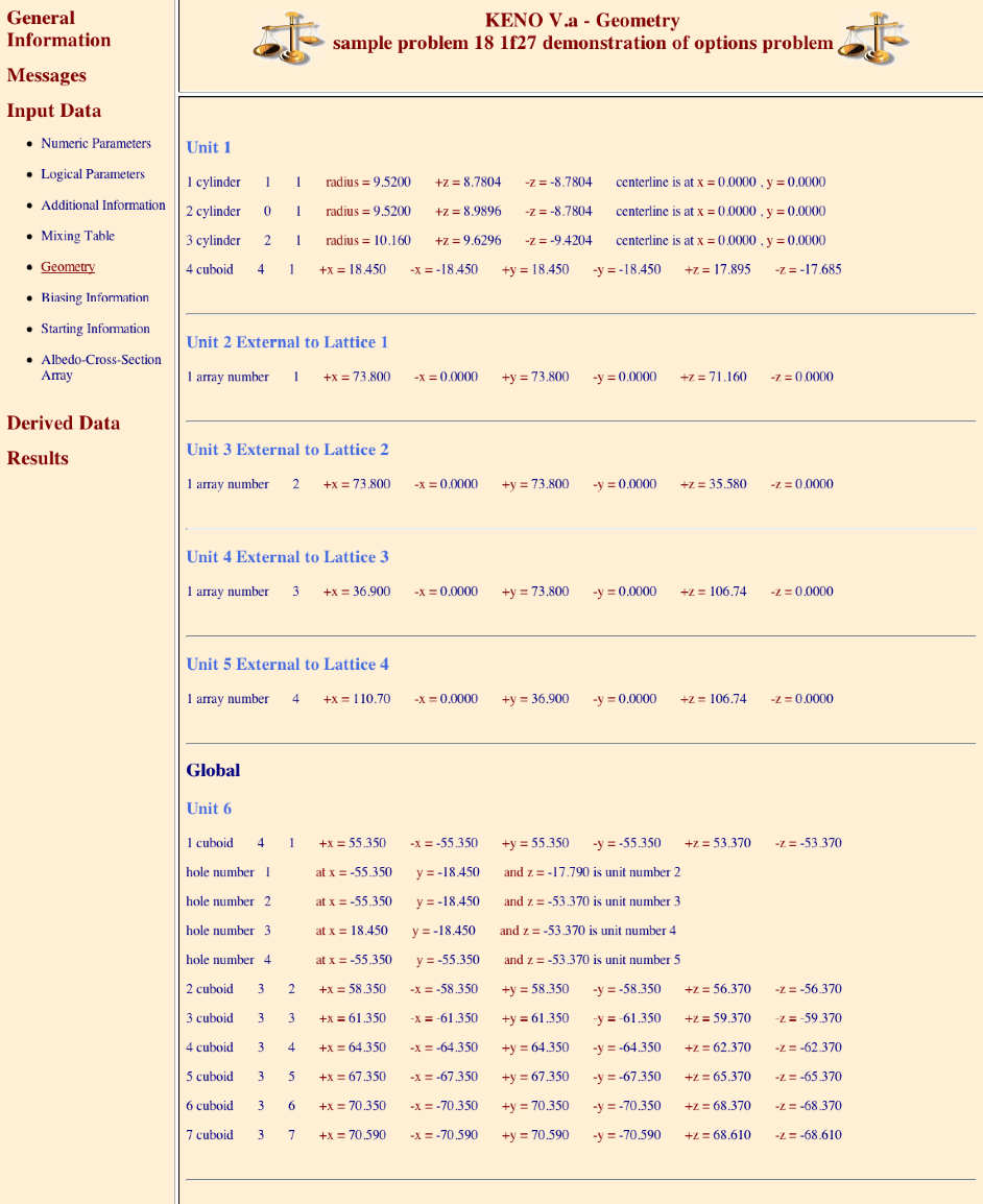
Fig. 8.1.180 Example of geometry region data in HTML output.

8.1.5.56.10. HTML output: Volume information

8.1.5.56.10.1. KENO V.a

Three tables of volumes are always printed. An example of the volume printout is given in Fig. 8.1.181. The HTML edit is accessed with the Volumes link in the Derived Data section.

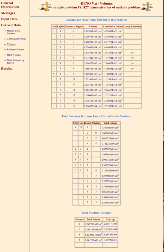
Fig. 8.1.181 Sample volume information in HTML output.

8.1.5.56.10.2. KENO-VI

Two tables of volumes are always printed. The first table will list the number of times each unit is used in the problem and the total volume of each region throughout the entire problem description. The second table will list the total volume and mass of each mixture used in the problem.

8.1.5.56.10.3. Mesh volumes

With the mesh flux accumulator, fluxes are tabulated for each region of each unit in a cubic mesh. For models in which the mesh flux accumulator is activated by setting MFX=YES and the mesh size set to a positive value with MSH=, the cumulative volume of all mesh intervals for a given region and the number of meshes used in each region are printed as shown in Fig. 8.1.182. The HTML edit is accessed with the Mesh Volumes link in the Derived Data section.

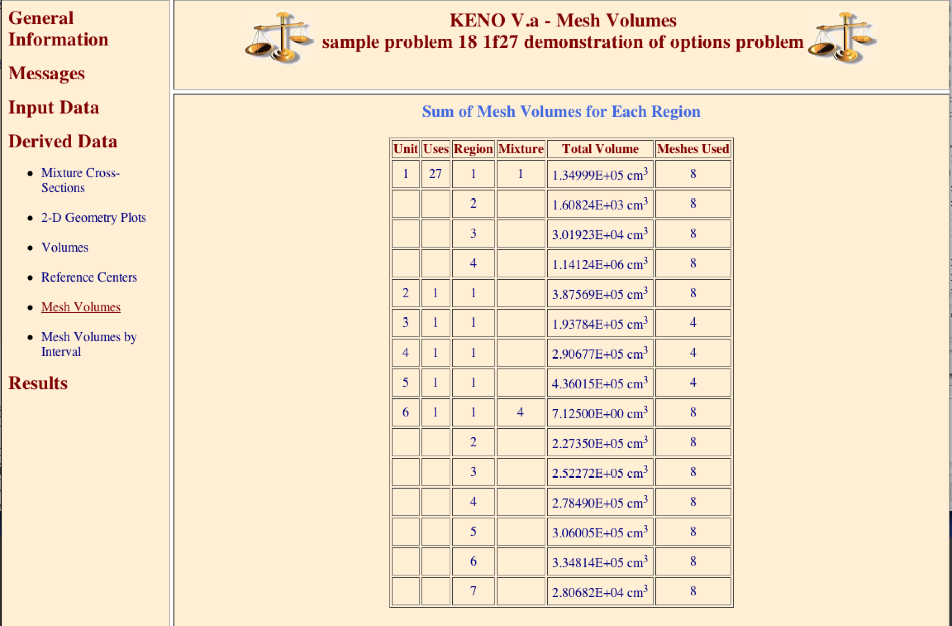
Fig. 8.1.182 Sample sum of mesh volumes in HTML output.

An optional edit of volumes for each mesh interval for each region can be activated by entering PMV=YES in the parameter input. This edit can be very large, especially if a small mesh size is used with a large model. A sample of the volume by mesh for each region is shown in Fig. 8.1.183. This edit is found under Derived Data with the Mesh Volumes by Interval link. For the HTML output, the links on the right side of the screen control what data are displayed in the center pane. Clicking on the unit number in the pane labeled UNIT places the pane labeled Region at that unit. Clicking on a region number in the region pane places the volume by mesh for the selected unit in the center pane.

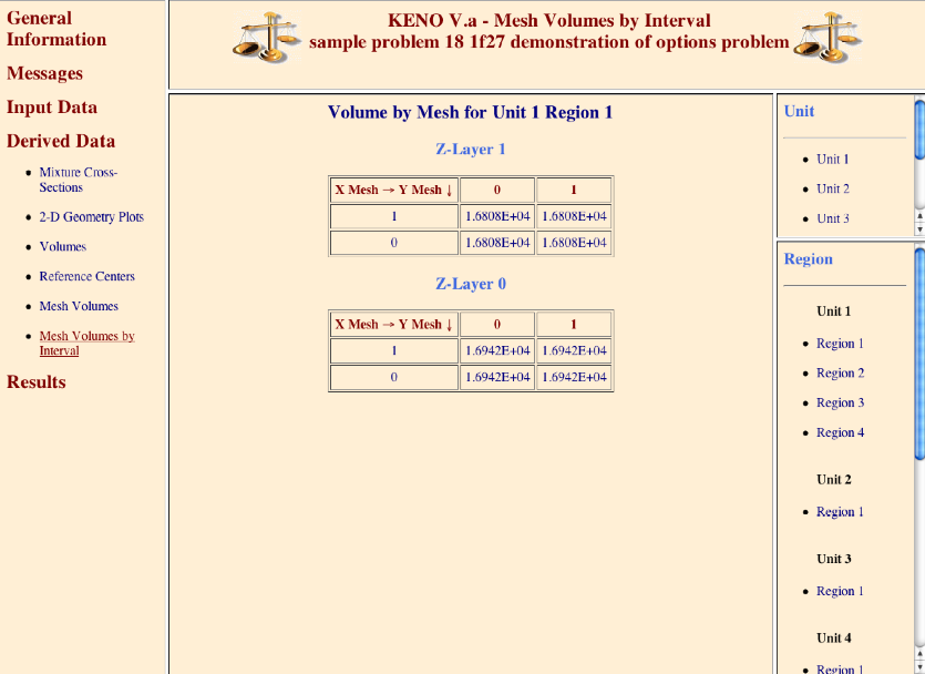
Fig. 8.1.183 Sample of volume by mesh for each region in HTML output.

8.1.5.56.11. HTML output: Biasing information

This table specifies the weighting or biasing data to be used in the problem. An example of biasing information is given in Fig. 8.1.184.

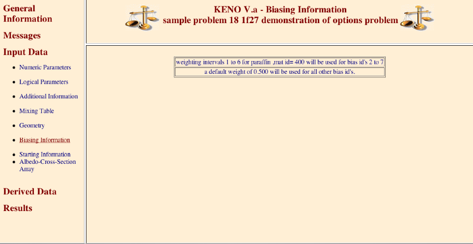
Fig. 8.1.184 Biasing information in HTML output.

8.1.5.56.12. HTML output: Group-dependent weights

Printing the group-dependent weights is optional. They are printed if PWT=YES is entered in the parameter data. This edit is available in the HTML output under Results in the Average Weight link, as shown in Fig. 8.1.185.

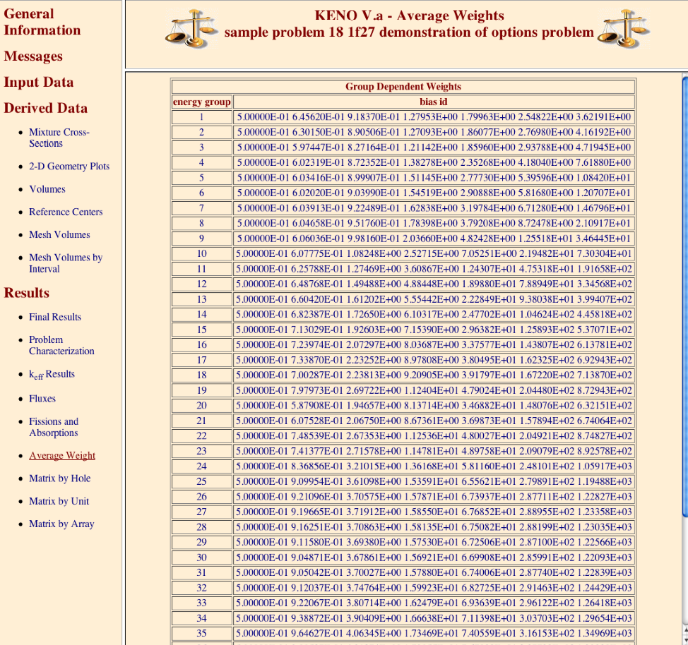
Fig. 8.1.185 Example of biasing data in HTML output.

8.1.5.56.13. HTML output: Plot representation

Plots representing 2-D slices through the geometrical description of the problem are optional. They are created if plot data are entered unless PLT=NO is specified either in the plot data or the parameter data. Character plots are not available in the HTML output, but the color plots are easily viewed as shown in Fig. 8.1.186. The user-requested plots can be viewed under Derived Data in the 2-D Geometry Plots link.

Fig. 8.1.186 shows two color plots in a single HTML page. The color plots do not appear in the KENO text printout, but they are an integral part of the HTML output. They are generated from PNG files created when a color plot has been specified in the KENO input data. Any number of plots can be made in one problem. The color plots can be valuable tools to assist the user in verifying that a problem is described correctly.

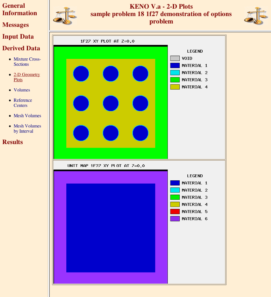
Fig. 8.1.186 Sample color plots in HTML output.

8.1.5.56.14. HTML output: Initial source and final pretracking edits

Prior to calculating the k-effs for each generation, KENO prints the final input data edit. The starting information is available in the HTML output under Input Data with the Starting Information link. An example of the HTML edit is shown in Fig. 8.1.187.

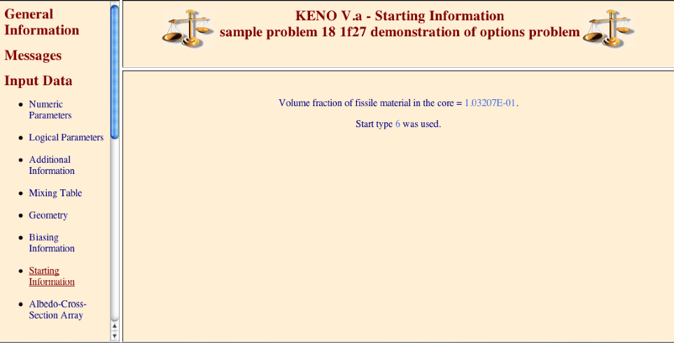
Fig. 8.1.187 Example of initial source information for start type 6 in HTML output.

8.1.5.56.15. HTML output: Reference center for flux moment/angular flux tranform

When TFM=YES is entered, the flux moments and angular fluxes are computed in a transformed coordinate system relative to a reference center point. Edits of the fuel center and the position of the reference center for each region are shown in Fig. 8.1.188. The HTML output edit is available under Derived Data in the Reference Centers link.

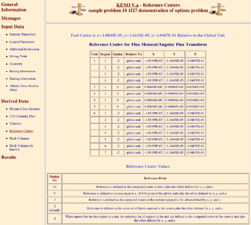
Fig. 8.1.188 Example of fuel center and reference center edits in HTML output.

8.1.5.56.16. HTML output: K-effectives by generation

At the completion of each generation, KENO prints the k-effective for that generation and associated information. An example of this printout is given in Fig. 8.1.188 for HTML output. This HTML output edit is available under Results in the section of keff Results in the keff by Generations Run link.

Example fuel center and reference center edits in HTML output.

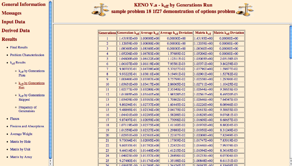
Fig. 8.1.189 Example of k-effective by generation in HTML output.

The problem title is printed at the top of the page. A descriptive heading is printed at the top of each column of data. The data printed include (1) the generation number, (2) the k-effective calculated for the generation, (3) the average value of k-effective through the current generation (excluding the first two generations), (4) the deviation associated with the average k-effective, and (5) the matrix k-effective for the generation and the deviation associated with the matrix k-effective. The last two columns are filled with zeros if the user did not specify matrix k-effective calculations. The matrix k-effective is the largest eigenvalue of the fission production matrix. Matrix information can be calculated based on (1) position index, (2) unit number, (3) hole number, and (4) array number. The matrix k-effective printed in the sixth column is based on this order. If the matrix k-effective is calculated by position index, it is the one printed in the sixth column. The matrix k-effective by unit number is given second preference, followed by hole number and then array number. After the last generation, a message is printed to indicate why execution was terminated. If matrix k-effectives were calculated, this is followed by a message stating the method used to determine the matrix k-effective.

The user should examine this portion of the results to ensure that the two methods of calculating k-effective are in acceptable agreement and to verify that the average value of k-effective has become relatively stable. If the k-effectives appear to be oscillating or drifting significantly, the user should consider rerunning the problem with a larger number of histories per generation.

If a problem is restarted, the generation numbers and k-effectives are printed and the words FROM RESTART UNIT are printed in the elapsed time column. All other columns are blank. When the generation at which the problem is to be restarted is reached, the print reverts to the normal format as shown in Fig. 8.1.137.

8.1.5.56.17. HTML output: Problem characterization edit

The problem characterization edit is shown in Fig. 8.1.190 for HTML output.

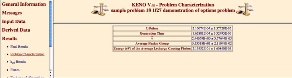
Fig. 8.1.190 Example problem characterization edit in HTML output.

8.1.5.56.18. HTML output: Final k-effective edit

The final k-effective edit prints the average k-effective and its associated deviation and the limits of k-effective for the 67, 95, and 99% confidence intervals. The final k-effective edit is printed as shown in Fig. 8.1.191. This HTML output edit is available under Results in the section of keff Results in the keff by Generations Skipped link.

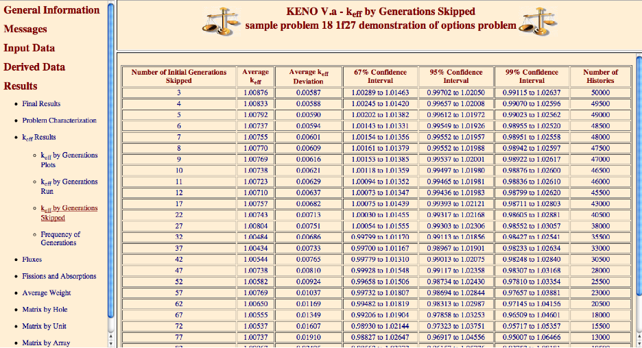
Fig. 8.1.191 Example of the final k-effective edit in HTML output.

8.1.5.56.19. HTML output: Final edit of fissions, absorptions, and leakage

The final edit of fissions, absorptions, and leakage follows the final k-effective edit and includes the fission fraction for each group and the fission production, absorptions, and leakage, each with its associated percent deviation.

Tables corresponding to those available in the text output are also available in the HTML output. These data are accessed with the Fissions and Absorptions Data link under Fissions and Absorptions in the Results section, as illustrated in Fig. 8.1.192, where the region and group data (FAR=YES and GAS=YES) are present. To allow quicker loading of the large amounts of data in the HTML output, the data have been subdivided into several separate tables, which are accessed with the menu on the right side of the window.

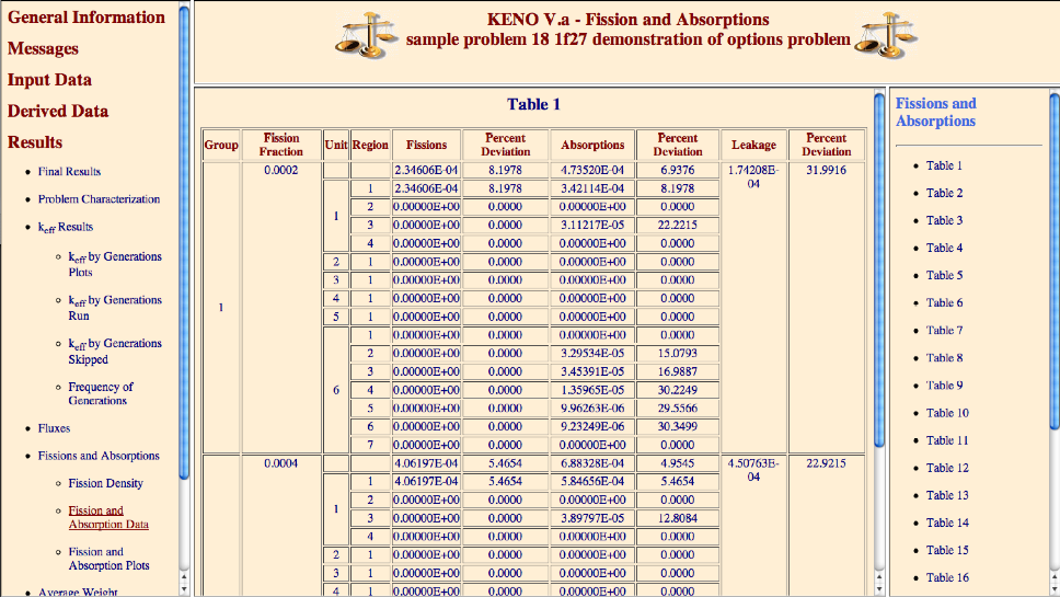
Fig. 8.1.192 Sample fissions, absorptions and leakage data in HTML output.

8.1.5.56.20. HTML output: Matrix k-effective by position index

The matrix k-effective by unit location (also referred to as array position or position index) is calculated if MKP=YES is specified in the parameter data and a global array is present in the model. An example of the matrix k-effective by position is given in Fig. 8.1.193. In the HTML output, the k-effective by position data is available in the Matrix by Position link in the Results section.

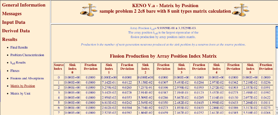
Fig. 8.1.193 Example of matrix k-effective by position index edit in HMTL output.

8.1.5.56.21. HTML output: Fission production by position index matrix

To obtain fission production by position information, the user must specify MKP=YES and FMP=YES in the parameter data. An example of the fission production matrix by position index for a 2 \(\times\) 2 \(\times\) 2 array is shown in Fig. 8.1.194.

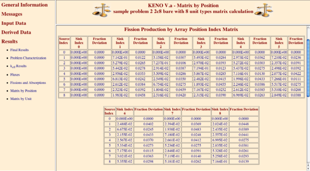
Fig. 8.1.194 Sample fission production matrix by position index edit in HMTL output.

For each position index in the array, the number of next-generation neutrons produced at position index J per neutron born at position index I is determined. The fission production matrix by position index is used to determine the matrix k-effective, cofactor k-effective and source vector by position index.

8.1.5.56.22. HTML output: Source vector by position index

Source vector by position index information is printed if MKP=YES is specified in the parameter data. An example of the source vector by position index is shown in Fig. 8.1.195. The average self-multiplication by array position is the overall average of the self-multiplication of all units used in the problem.

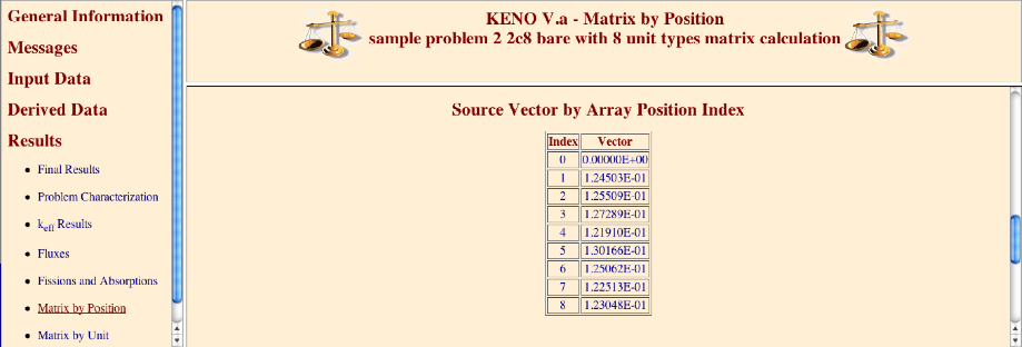
Fig. 8.1.195 Example of source vector by position index edit in HTML output.

8.1.5.56.23. HTML output: Cofactor k-effective by position index

The cofactor k-effective by position index edit is printed if MKP=YES is specified in the parameter data. An example of the cofactor k-effective by position index is shown in Fig. 8.1.196 and an example of the source vector by position index is shown in Fig. 8.1.197.

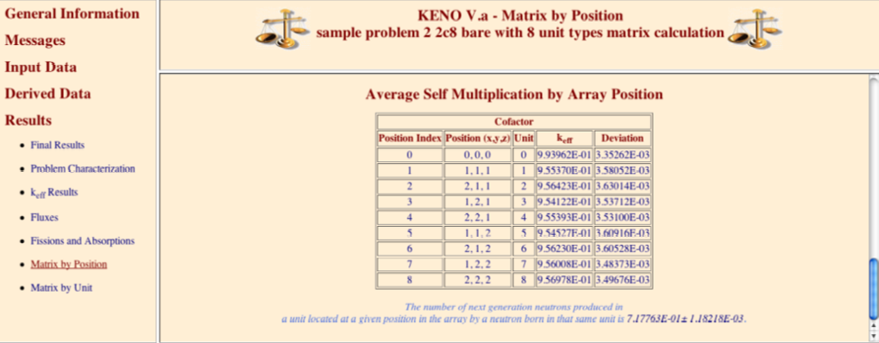
Fig. 8.1.196 Example cofactor k-effective by position index edit in HTML output.

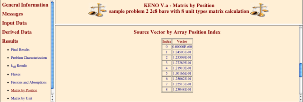
Fig. 8.1.197 Example of source vector by position index edit in HTML output.

8.1.5.56.24. HTML output: Matrix k-effective, fission production, source vector and cofactor k-effective by unit number

The matrix k-effective by UNIT number (unit k-effective) is the largest eigenvalue of the fission production by unit matrix. It is calculated only if MKU=YES is specified in the parameter data. An example of the matrix k-effective by UNIT is given in Fig. 8.1.198. Fission production, source vector and average self-multiplication by UNIT are all printed on the same page as the matrix k-effective by UNIT. The matrix k-effective HTML data by unit is available in the Matrix by Unit link in the Results section.

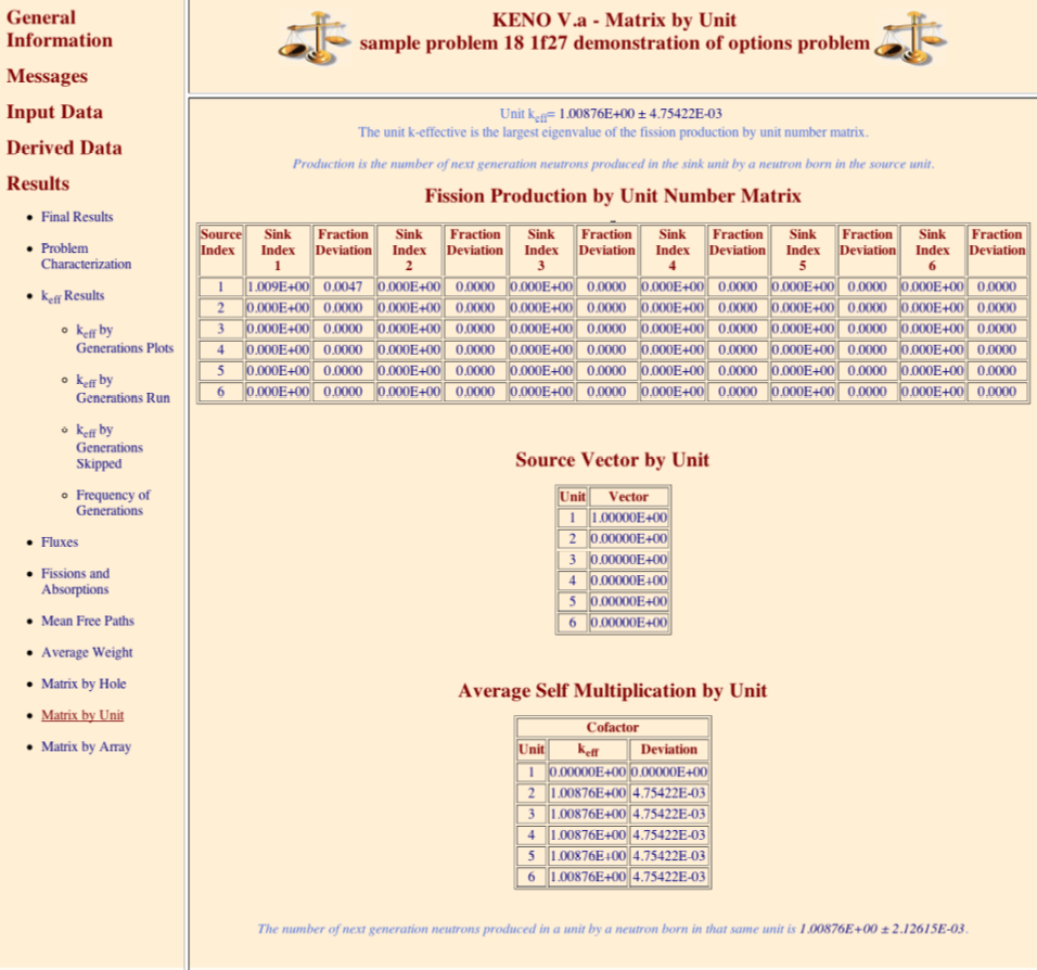
Fig. 8.1.198 Example matrix by unit edit in HTML output.

8.1.5.56.25. HTML output: Matrix k-effective, fission production, source vector and cofactor k-effective by hole number

The matrix k-effective by HOLE number is the largest eigenvalue of the fission production matrix collected by HOLE number and is calculated if MKH=YES was specified in the parameter data. An example of the matrix k-effective by HOLE number is given in Fig. 8.1.199. Fission production, source vector and average self-multiplication by HOLE are all printed on the same page as the matrix k-effective by HOLE. The matrix k-effective HTML data by HOLE is available in the Matrix by Hole link in the Results section.

Fig. 8.1.199 Example matrix k-effective by hole edit in HTML output.

8.1.5.56.26. HTML output: Matrix k-effective, fission production, source vector and cofactor k-effective by array number

The matrix k-effective by array number is the largest eigenvalue of the fission production matrix collected by array number and is calculated if MKA=YES is entered in the parameter data. The number of next generation neutrons produced in array number J by a neutron born in array number I is given in this fission production matrix.

The matrix k-effective HTML data by array is available in the Matrix by Array link in the Results section, with an example shown in Fig. 8.1.200. Fission production, source vector and average self-multiplication by ARRAY number are all printed on the same page as the matrix k-effective by ARRAY number.

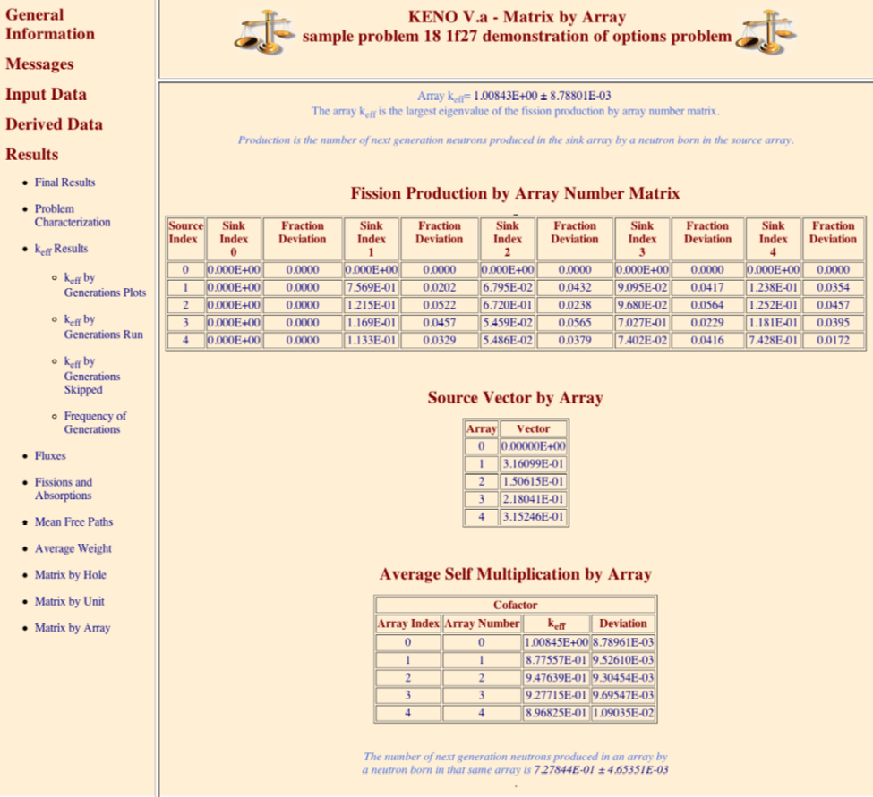
Fig. 8.1.200 Example matrix by array edit in HTML output.

8.1.5.56.27. HTML output: Fission density edit

The fission density edit is optional. In the HTML output, the fission density edit is available in the Fission Density link of Fissions and Absorptions under the Results section, as shown in Fig. 8.1.201.

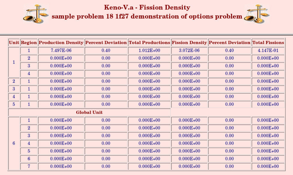
Fig. 8.1.201 Example fission density edit in HTML output.

8.1.5.56.28. HTML output: Flux edit

Printing the fluxes is optional; they are only printed if FLX=YES is specified in the parameter data. The fluxes are printed for each unit and each geometry region in the unit for every energy group.

In the HTML output, a table of flux data can be accessed with the Scalar Fluxes under Fluxes in the Results section, as shown in Fig. 8.1.202. The fluxes for each unit in the problem are accessed from links on the right side of the page. Separate links are presented for Angular Fluxes and Flux Moments if they are requested in the problem.

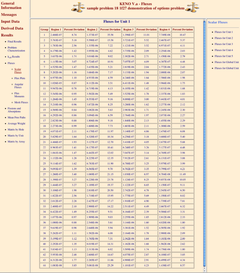
Fig. 8.1.202 Example scalar flux edit in HTML output.

8.1.5.56.29. HTML output: Final results table

The final results table contains a summary of the most important physics parameters of the system and the number of error and warning messages generated during execution.

In the HTML output, the final results table is accessed with the Final Results link in the Results section, as shown in Fig. 8.1.203.

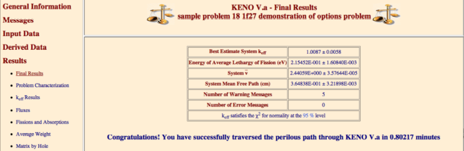
Fig. 8.1.203 An example of the final results table in HTML output.

8.1.6. Warning messages and error messages

KENO prints warning and error messages that are identified by K5- or K6- for KENO V.a and KENO-VI, respectively, followed by a unique number (i.e., K5-001 is the identifier of the first message for KENO V.a). The generic symbol for messages originating in KENO V.a and KENO-VI is K?, where the question mark stands for 5 or 6. For additional information concerning the message, refer to the identifier number in this section.

Warning messages appear when a possible error is encountered. If the code alters data, that fact is stated in the message. It is the responsibility of the user to verify correct usage when a warning message is printed.

When an error is encountered, a global error flag (MFLAG) is set true and an error message is printed. The code immediately stops or execution is terminated with an error code if the error is too severe to continue. The warning and error messages in this section may show an underscore ____ or a numbered underscore (1) where data will be printed by the code. The explanation of the message will show an underscore or a numbered underscore to indicate the corresponding data.

8.1.6.1. Messages

KMSG001

*** WARNING *** K?-001 FOLLOWS:
READ FLAG NOT FOUND. ASSUME PARAMETER DATA FOLLOWS.

This message occurs in subroutine INITAL. It indicates that the word READ was not the first word of data encountered after the title card. If a parameter data block is to be entered, the code expects the words READ PARAMETERS to precede the parameter input data. If the word READ is not the first word, the code expects parameter input data immediately.

KMSG002

** ERROR ** K?-002 FOLLOWS:
THE NUMBER OF ENERGY GROUPS IS OUT OF RANGE FOR THE CROSS SECTION LIBRARY ON UNIT ___ THE INPUT MAY NOT SPECIFY A VALID DATA SET ON THIS UNIT OR THE MODULE THAT WAS TO CREATE THE CROSS SECTION LIBRARY ON THIS UNIT MAY HAVE FAILED

This message occurs in subroutine INITAL after subroutine PARAM has been executed. Unit number ____ should be checked to ensure that it was properly specified in the job control language. The data set name associated with this unit number should also be verified. This information is given in the printout in the third table. The module that generated the cross sections should be verified as having executed properly and that the data were saved or passed correctly. When this message is printed for an AMPX working format library, a STOP 108 is executed. When this message is printed for a mixed cross section format library, a STOP 109 is executed.

KMSG003

*** WARNING *** K?-003 FOLLOWS:
MAT ID=___ WAS NOT FOUND IN THE WEIGHTS LIBRARY FOR THE SPECIFIED ENERGY GROUP STRUCTURE.

This message is printed in subroutine LODWTS when loading biasing factors from the direct access scratch file. It indicates that weights library did not contain biasing factors for this ID for the group structure that corresponds to the cross sections (multigroup), or to the binning structure (continuous energy). Default biasing factors will be substituted. The location of this set of biasing parameters should be checked to verify that the substitution does not cause a problem.

KMSG004

*** ERROR *** K?-004 FOLLOWS:
INVALID INPUT PARAMETER NAME ___

This message comes from subroutine PARAM and indicates that the keyword for entering parameter data was misspelled or in error in some other way. A list of allowed keywords is given in Table 8.1.1 in the KENO input outline.

KMSG005

*** ERROR *** K?-005 FOLLOWS:
AN ERROR WAS ENCOUNTERED IN THE ALPHANUMERIC PARAMETER DATA. THE DATA WAS ___

This message comes from subroutine PARAM and indicates that the keyword for the alphanumeric parameter data was entered correctly, but the data associated with it were not YES or NO as is required. The____ ____ in the error message could be something like FLX=YEX instead of FLX=YES.

KMSG006

** WARNING ** K?-006 FOLLOWS:
READ FLAG FOUND WHEN LOOKING FOR END FLAG. PARAMETER INPUT ASSUMED COMPLETE

This message occurs in subroutine PARAM. It indicates that the keywords END PARAMETERS were not found. The keywords READ____ were found instead. The code assumes the parameter data are complete and proceeds normally.

KMSG007

** ERROR ** K?-007 FOLLOWS:
ATTEMPT TO FIND END PARAMETER FLAG WAS UNSUCCESSFUL.

This message from subroutine PARAM occurs during the reading of the parameter data if the word END is found and it is not followed by the word PARAMETERS. A STOP 118 may be executed when this message is printed.

KMSG008

** ERROR ** K?-008 FOLLOWS:
AN END OF FILE WAS ENCOUNTERED WHILE ATTEMPTING TO READ PARAMETER DATA

This message is from subroutine PARAM. A STOP 118 may be executed when this message is printed.

KMSG009

** WARNING ** K?-009 FOLLOWS:
DUE TO INCONSISTENCIES BETWEEN INPUT AND RESTART DATA, FISSIONS AND ABSORPTIONS BY REGION WILL BE CALCULATED BUT NOT PRINTED. INPUT DATA SET FAR=NO, BUT DATA FROM THE RESTART UNIT SPECIFIED YES.

This message occurs in subroutine PARTBL and is mostly self-explanatory. The original problem (parent case) that wrote the restart data specified data inconsistent with the parameter data input to the restarted problem. The title of the parent case is given at the end of the parameter tables. The specification of the restart unit RST is given in the third table of the KENO output.

KMSG010

*** WARNING *** K?-010 FOLLOWS:
DUE TO INCONSISTENCIES BETWEEN INPUT AND RESTART DATA, FLUXES WILL BE CALCULATED BUT NOT PRINTED. INPUT DATA SET FLX=NO, BUT DATA FROM THE RESTART UNIT SPECIFIED YES.

This message occurs in subroutine PARAM. The original problem (parent case) that wrote the restart data specified data did not agree with the parameter data input to the restarted problem. The title of the parent case is given at the end of the parameter tables. The specification of the restart unit RST is given in the third table of the KENO output.

KMSG011

** ERROR ** K6-011 FOLLOWS:
A BOUNDARY GEOMETRY WORD WAS NOT SPECIFIED FOR UNIT ___

This KENO-VI message is from subroutine SGGM_KENOG. A BOUNDARY card must be associated with each unit identifying the outermost region of the unit.

KMSG012

** WARNING ** K?-012 FOLLOWS:
INPUT PARAMETER NBK WAS ENTERED AS ___. IT WAS CHANGED TO ___. AT LEAST ___ POSITIONS ARE NECESSARY TO ACCOMMODATE THE NEUTRON BANK DATA.

This self-explanatory message is from subroutine PARTBL. NBK should not be entered as input data unless it is known that the default value is inadequate.

KMSG013

** ERROR ** K6-013 FOLLOWS:
MEDIA DATA MUST BE ENTERED FOR UNIT ___

This KENO-VI message is from subroutine SGGM_KENOG. Either another UNIT card or an END GEOM card was encountered prior to inputting MEDIA data for the current unit.

KMSG014

** ERROR ** K?-014 FOLLOWS:
ERROR - KEYWORD ___ ___ IS NOT A VALID MIXING TABLE KEYWORD.

This message is from subroutine MIXING_TABLE. It can only be encountered if a mixing table is expected (i.e., READ MIX or READ MIXT has been entered as data). At this point the only valid keywords are MIX=, EPS=, SCT= or NCM=. The keyword that was entered is printed in the message. See Sect. 8.1.3.10 for assistance in setting up the mixing table data.

KMSG015

** ERROR ** K5-015 FOLLOWS:
AN ERROR WAS FOUND IN THE HEMISPHERE DESIGNATION

This KENO V.a message was printed by subroutine K5GM_KENOG. It signifies that the geometry keyword has been destroyed after it was read. This indicates a code bug.

KMSG016

*** ERROR *** K?-016 FOLLOWS:
** ERROR ** A VALUE MUST BE ENTERED FOR LIB IN THE PARAMETER INPUT SO CROSS SECTIONS CAN BE MIXED.

This message is from subroutine DATAIN. It occurs when a mixing table has been read but the unit number for the AMPXS working library is undefined. This is corrected by entering LIB=____ in the parameter input data and making sure the desired AMPXS working library is properly defined as being on that unit in the job control language.

KMSG017

*** ERROR *** K?-017 FOLLOWS:
UNRECOGNIZABLE GEOMETRY WORD ___

This message is from subroutines K5GM_KENOG, SGGM_KENOG, K5GM_CENTER or SGGM_CENTER. In the process of reading the geometry data, the word ____ was encountered when a geometry word was expected. Several of these messages may be generated. A message is generated for each word of data that is read, until a valid geometry word is found. The data are out of phase or the geometry word is misspelled. The previous geometry word should be checked to ensure that it has the correct entries. See Sect. 8.1.8.1 and Sect. 8.1.8.2 for lists of accepted geometry words.

KMSG018

***** ERROR ***** K6-018 FOLLOWS:
INVALID INDEX INTO KEYWRD ARRAY. INP=___ CHECK SUBROUTINE KENOG FOR A CODE ERROR.

This KENO-VI message is from subroutine SGGM_KENOG. This message usually means that a code error was introduced when changes were made to the program. Subroutine KENOG, function LCOMPR, and KEYWRD data block should be checked.

KMSG019

***** ERROR ******** ERROR ******** ERROR ******** ERROR ******** ERROR ******** ERROR ******** ERROR ******** ERROR ******** ERROR ******** ERROR ****
K6-019 FOLLOWS: A GLOBAL UNIT HAS NOT BEEN SPECIFIED.
**** ERROR ******** ERROR ******** ERROR ******** ERROR ******** ERROR ******** ERROR ******** ERROR ******** ERROR ******** ERROR ******** ERROR ****

This KENO-VI message from subroutine SGGM_KENOG indicates that a GLOBAL UNIT has not been specified. The outermost unit in the problem must be specified as the GLOBAL UNIT. See Sect. 8.1.3.4 to determine the correct specification.

KMSG020

*** ERROR *** K6-020 FOLLOWS:
GEOMETRY WORD INDEX OUT OF RANGE ON SCRATCH UNIT ___ FOR GEOMETRY WORD NUMBER ___ INP=___ GWRD=___

This KENO-VI message from subroutine SGGM_READGM means that INP is negative or larger than NP when the geometry data are read from the scratch unit, SKRT. This usually means that a code error was introduced when changes were made to the program. True geometry errors should be detected when the scratch unit, SKRT, is written. A STOP 125 is executed when this message is printed.

KMSG021

*** ERROR *** K?-021 FOLLOWS:
___ IS AN INVALID PARAMETER NAME FOR BIASING DATA. ID= OR WT= OR WTS= SHOULD HAVE BEEN ENTERED.

This message is from subroutine RDBIAS. See Sect. 8.1.3.7 for assistance in determining the proper procedure for entering biasing data.

KMSG022

*** ERROR *** K?-022 FOLLOWS:
PROBLEM IN READGM, IGEO=___ IS AN INVALID GEOMETRY TYPE

If this message has not been preceded by other geometry error messages, it indicates a code bug.

KMSG023

*** ERROR *** K5-023 FOLLOWS:
REFLECTION OR PERIODIC BOUNDARY CONDITIONS ARE ILLEGAL ON A CURVED BOUNDARY.

This self-explanatory KENO V.a message from K5GM_JOMCHK indicates that only a vacuum or a white boundary condition is allowed on a curvilinear surface.

KMSG024

K?-024 FOLLOWS:
INCORRECT FLAG RETURNED FROM AREAD. IRET=___

This message from subroutine RDBIAS indicates that an error was encountered while reading the biasing data. The biasing data were not entered properly. See Sect. 8.1.3.7 for assistance.

KMSG025

*** ERROR *** K5-025 FOLLOWS:
WHITE BOUNDARY CONDITION IS ALLOWED ONLY ON CUBOIDS, CYLINDERS, OR SPHERES

This self-explanatory KENO V.a message from K5GM_JOMCHK indicates that WHITE albedo boundary conditions cannot be applied to the outermost geometry if it is a hemisphere or a hemicylinder.

KMSG026

K?-026 - ARRAY DESCRIPTION ERROR MESSAGES
K?-026 FOLLOWS:
SET NUMBER ___ OF THE UNIT ORIENTATION DATA CONTAINS ___ ERROR(S).

This message from subroutine RDBOX is triggered when input errors are recognized in the unit orientation data. A set of unit orientation data consists of 10 numbers as shown in the companion message KMSG027. The number of errors printed in this message is a lower bound. More errors may actually exist. This message often means that a number was omitted or a blank was omitted when entering the unit orientation data.

KMSG027

K?-027 FOLLOWS:
LTYPE=___ IX1=___ IX2=___ INCX=___ IY1=___ IY2=___ INCY=___ IZ1=___ IZ2=___ INCZ=___

This message is a companion to KMSG026. It indicates how the unit orientation data description for the set named in KMSG026 was entered. See Sect. 8.1.3.5.2 for information pertaining to unit orientation data.

KMSG028

K?-028 FOLLOWS:
THE ABOVE UNIT ORIENTATION CARD(S) CONTAIN(S) AT LEAST ONE OF THE FOLLOWING ERRORS.
1. IX1, IY1, IZ1, INCX, INCY, OR INCZ IS LESS THAN OR EQUAL TO ZERO
2. IX2 IS LESS THAN IX1, IY2 IS LESS THAN IY1, OR IZ2 IS LESS THAN IZ1
3. IX2 IS GREATER THAN NBXMAX, IY2 IS LARGER THAN NBYMAX, OR IZ2 IS LARGER THAN NBZMAX
4. LTYPE IS LESS THAN 1 OR GREATER THAN NBOX

This self-explanatory message is from subroutine RDBOX. It pertains to the input orientation data for LOOP. See Sect. 8.1.3.5 for input instructions.

KMSG029

*** ERROR *** K?-029 FOLLOWS:
THE ARRAY SIZE HAS BEEN SPECIFIED INCORRECTLY. NBXMAX=___ NBYMAX=___ NBZMAX=___ UNIT ORIENTATION DATA CANNOT BE READ UNLESS NBXMAX, NBYMAX AND NBZMAX ARE GREATER THAN ZERO.

This message from subroutine ARAYIN indicates that the array definition data were incorrectly specified. It occurs only if one or more of NBXMAX, NBYMAX, or NBZMAX is less than 1. In the array information data these are entered in the form NUX=____ NUY=____ NUZ=____. See Sect. 8.1.3.5. If a unit orientation data description is to be entered, NBXMAX, NBYMAX, and NBZMAX must all be greater than zero.

KMSG030

*** ERROR *** K?-030 FOLLOWS:
END ___ FLAG WAS NOT FOUND. ___ ___ WAS READ INSTEAD.

This message from subroutine ARAYIN occurs if the unit orientation data description is terminated with the incorrect END flag.

KMSG031

*** ERROR *** K?-031 FOLLOWS:
___ IS AN INVALID PARAMETER NAME IN THE ARRAY DATA.

This message is written from subroutine ARAYIN if the array data block contains an incorrect keyword. The allowed keywords include NUX=, NUY=, NUZ=, FILL, LOOP, ARA``* =, ``TYP =. See Sect. 8.1.3.5 for additional assistance. A STOP 101 is executed when this message is printed.

KMSG032

`` ERROR `` K?-032 FOLLOWS:
AN ERROR EXISTS IN UNIT ORIENTATION ARRAY NUMBER ___

This message from subroutines K5_SORTA or K6_SORTA is printed when an error is recognized in the array description. The type of error that will trigger the message is for a position in the unit orientation array to be undefined, zero, negative or greater than NBOX, the largest unit number. KMSG033 is a companion message.

KMSG033

*** ERROR *** K?-033 FOLLOWS:
UNIT ___ IS INVALID AT X INDEX =___ Y INDEX =___ Z INDEX =___

This message comes from subroutines K5_SORTA or K6_SORTA. It is printed for each position in the unit orientation array that is in error. The message is printed a maximum of 10 times. Refer to Sect. 8.1.3.5 for assistance in correcting the error(s).

KMSG034

*** ERROR *** K?-034 FOLLOWS:
THE NUMBER OF MIXTURES REQUESTED IN THE GEOMETRY IS ___ THE NUMBER OF MIXTURE CROSS SECTIONS IS ___

This message from subroutines K5_FLDATA, K6_FLDATA or MFLDATA occurs if the number of mixture cross sections from the restart unit, RSTRT, does not equal the number of mixtures requested in the geometry for a restarted problem.

KMSG035

*** ERROR *** K?-035 FOLLOWS:
IN THE ALBEDO INPUT DATA ___ IS AN INVALID FACE CODE NAME.

This message is from subroutine RDREF. It occurs if an invalid face code name was entered in the albedo data. See Table 8.1.20 in Sect. 8.1.3.6 for a list of acceptable face code names.

KMSG036

*** ERROR *** K6-036 FOLLOWS:
A BOUNDARY BODY ___ WAS SPECIFIED THAT IS NOT ONE OF THE BODIES IN THE GLOBAL UNIT BOUNDARY.

This message is from subroutines K6_RDBNDS or LOADGEOM1. It indicates that a boundary body was specified to assign boundary conditions that do not exist in the global unit. The bodies specified for boundary conditions should be carefully matched with those specified in the boundary definition vector of the global unit.

KMSG037

**** ERROR ***** K?-037 FOLLOWS:
AVERAGE NU-BAR AND AVG. FISSION GROUP WAS SPECIFIED, BUT THE FISSION XSEC ID (18) WAS NOT FOUND IN THE EXTRA 1-D ARRAY (MT).

This message is from subroutine IDX1D. It indicates that the parameter data contained NUB= YES, but the corresponding necessary type of data was absent from the extra 1-D array. This can be due to a code error or an error concerning the extra 1-D data (X1D= in the parameter data).

KMSG038

**** ERROR *** K?-038 FOLLOWS:
INPUT DATA INDICATED NO EXTRA 1-D XSEC IDS TO BE READ, BUT A READ FLAG WAS ENCOUNTERED.

This message from subroutine DATAIN is printed when the parameter data did not specify X1D= and the words READ X1DS were encountered later in the data. If extra 1-D data are to be used, X1D= must be entered in the parameter data and appropriate code modifications must be made to properly use the extra 1-D data.

KMSG039

*** ERROR *** K?-039 FOLLOWS:
INVALID START PARAMETER NAME ___

This message is from subroutine RDSTRT. It indicates that an invalid start parameter name was encountered when the start data block was being read. A list of allowed start parameter names is contained in Sect. 8.1.3.8.

KMSG040

*** WARNING *** K?-040 FOLLOWS:
LNU FOR START TYPE 6 WAS ENTERED AS ___. THE LARGEST VALUE NEEDED FOR LNU IS NPG; ENTRIES BEYOND NPG WILL BE IGNORED.

This self-explanatory message is from subroutine RDSTRT. See Sect. 8.1.3.8 and Sect. 8.1.4.8 for assistance in determining a valid value for LNU. NPG, the number of histories per generation, starting neutrons are needed to fill the initial neutron bank. KENO discards the starting points beyond NPG and notifies user with this message about this action.

KMSG041

*** ERROR *** K?-041 FOLLOWS:
ALPHANUMERIC START DATA MUST BE ENTERED AS YES OR NO. THE DATA READ WAS ___ ___

This self-explanatory message is from subroutine RDSTRT. See Sect. 8.1.3.8 for assistance concerning start data.

KMSG042

*** WARNING *** K?-042 FOLLOWS:
END ___ FLAG WAS NOT FOUND.___ ___ WAS READ INSTEAD

This message occurs when the READ ____ and END ____ do not match. When entering data blocks, each block must start with READ ____ and end with END ____.

KMSG043

*** ERROR *** K?-043 FOLLOWS:
AN END OF FILE WAS ENCOUNTERED BEFORE AN END DATA WAS FOUND. THE PROBLEM WILL NOT RUN.

This message is from subroutine DATAIN. It occurs when an end of file is encountered while reading data.

KMSG044

*** ERROR *** K?-044 FOLLOWS:
A PLOT OF ZERO HEIGHT AND/OR WIDTH HAS BEEN SPECIFIED.
THE HEIGHT IS ___ AND THE WIDTH IS ___
THE DELTA X IS ___, THE DELTA Y IS ___, AND THE DELTA Z IS ___
THE DIRECTION COSINES DOWN THE PAGE ARE ___ ___ ___
THE DIRECTION COSINES ACROSS THE PAGE ARE ___ ___ ___

This message is from subroutine RDPLOT. At least one of the X, Y, or Z components that make up the upper left corner and lower right corner is inconsistent or one of the direction cosines UAX, VAX, WAX, UDN, VDN, or WDN have the wrong sign. Check the plot data for consistency.

KMSG045

*** ERROR *** K?-045 FOLLOWS:
ILLEGAL DATA BLOCK IDENTIFIER, ___ ___

This message from subroutine DATAIN is printed whenever an invalid data block identifier is encountered. This can be caused by having the data out of order, by omitting data or by misspelling data. A block identifier consists of the words READ XXXX where XXXX is a keyword identifying the type of data to be read. Acceptable keywords when running KENO stand-alone are listed in Sect. 8.1.3.1.

KMSG046

*** ERROR *** K?-046 FOLLOWS:
IPT=___ IS OUTSIDE THE ALLOWABLE LIMIT OF ___

This message is from subroutine DATAIN. It is indicative of a code error. IPT is the index into the LPOINT array, which contains the direct access pointers for the various types of data.
LPOINT(1) is the pointer for the geometry region data.
LPOINT(2) is the pointer for the array description (unit orientation) data.
LPOINT(3) is the pointer for the mixing table data.
LPOINT(4) is the pointer for volume data.
LPOINT(5) is the pointer for the biasing or weighting data.
LPOINT(6) is the pointer for the start data.
LPOINT(7) is the pointer for the albedo data.
LPOINT(8) is the pointer for the mixed cross section data.
LPOINT(9) is the pointer for the energy and inverse velocity data.
LPOINT(10) is the pointer for the plot data.
LPOINT(11) is the pointer for the biasing input data.
LPOINT(12) is the pointer for the grid data for fluxes.
LPOINT(13) is the pointer for importance mapping data.
LPOINT(14) is the pointer for reactions data.
LPOINT(15) is the pointer for definitions data.
LPOINT(16) is the pointer for system responses data.
LPOINT(17) is the pointer for tallies data.
LPOINT(18) is the pointer for the albedo-xsec energy correspondence data.

A STOP 152 is executed when this message is printed.

KMSG047

***** ERROR ***** K6-047 FOLLOWS:
SECTOR DATA WAS NOT FOUND FOR ARRAY ___

This KENO-VI message is from subroutine SGGM_ARRAY. This message usually means that sector data was left off the ARRAY contents record. See Sect. 8.1.3.4 for assistance in specifying an ARRAY.

KMSG048

*** ERROR *** K?-048 FOLLOWS:
UNABLE TO ALLOCATE ___ DUE TO ERROR STATUS CODE ___ IN SUBROUTINE ___

This message is associated with allocating memory used to store problem dependent data. The message states the type of data memory was allocated for the error type returned when memory could not be allocated and the current subroutine. This message could be caused by insufficient system memory or a code problem.

KMSG050

*** ERROR *** K6-050 FOLLOWS:
THE ___ POSITION OF ARRAY ___ IN UNIT ___ WAS SPECIFIED AS ___ WHICH IS LESS THAN 1 OR GREATER THAN ___, THE NUMBER OF UNITS IN THAT DIRECTION.

This self-explanatory KENO-VI message from subroutine SGGM_CORSIZ indicates that an array was not properly placed in a unit. This is usually due to the incorrect definition of one of the array indices in one dimension (X, Y, or Z) such that it was specified outside the array bounds in that dimension.

KMSG051

*** ERROR *** K?-051 FOLLOWS:
SURFACE ___ OF BOUNDARY LABEL ___ REQUESTED A DIFFERENTIAL ALBEDO THAT IS NOT ON THE ALBEDO DATA SET. THE REQUESTED ALBEDO NAME IS ___

This message is from subroutine ALBRD. A list of the albedos that are on the standard albedo data set is given in Table 8.1.23 (Sect. 8.1.3.6).

KMSG052

*** ERROR *** K?-052 FOLLOWS:
INTERPOLATION CODE SHOULD BE IN THE RANGE 1 TO 5
INT: ___

This message is from subroutine XSEC_INTERP. This indicates an error in the continuous energy point data. INT is the interpolation code from the data. A STOP 104 is executed in conjunction with this message, and a traceback may be printed from subroutine STOP.

KMSG053

*** ERROR *** K?-053 FOLLOWS:
LOG INTERPOLATION SHOULD NOT BE USED WITH NEG OR ZERO ARGUMENT
XP: ___

This message is from subroutine XSEC_INTERP and indicates that a LIN-LOG interpolation was requested with a non-positive value. A STOP 104 is executed in conjunction with this message, and a traceback may be printed from subroutine STOP.

KMSG054

*** ERROR *** K?-054 FOLLOWS:
A SURFACE NUMBER ___ WAS SPECIFIED THAT IS LARGER THAN NUMBER OF SURFACES IN THE INDICATED GLOBAL BODY. THE PROBLEM WILL NOT BE RUN.

This message is from subroutines K5_RDBNDS or K6_RDBNDS. It indicates that an incorrect surface was specified to which a boundary condition was to be assigned. The surfaces of the bodies specified for boundary conditions should be carefully matched with those specified in the bounds of the global unit. Corresponding albedo surface numbers for all geometric shapes supported by KENO V.a and KENO-VI are listed in Table 8.1.21 and Table 8.1.22, respectively.

KMSG056

*** ERROR *** K?-056 FOLLOWS:
MIXTURE ___ LACKS EITHER NU*FISSION OR CHI DATA

This message from subroutines NORM1D or XSEC1D indicates that a mixture that contains fissile material is missing the nu-fission cross section or the fission spectrum. A STOP 115 is executed when this message is printed.

KMSG057

*** ERROR *** K5-057 FOLLOWS:
INVALID BIAS ID ___ IN REGION ___ ABOVE.

This KENO V.a message is from subroutines K5GM_PRTJOM or K5GM_READGM. It is printed if a negative or zero bias ID is entered for the specified geometry region. Review Sect. 8.1.3.4 for correct geometry data specification information.

KMSG058

*** ERROR *** K6-058 FOLLOWS:
INVALID BIAS ID IN REGION ABOVE.

This KENO-VI message is from subroutine SGGM_PRTJOM. It is printed if a negative or zero bias ID is entered for the specified geometry region. Review Sect. 8.1.3.4 for correct geometry data specification information.

KMSG059

*** ERROR *** K?-059 FOLLOWS:
THE CALCULATION WAS TERMINATED BECAUSE OF EXCESSIVE SPLITTING.

This message from subroutines K5_GUIDE or K6_GUIDE is printed only if message K?-128 is printed 50 or more times for a given generation. This indicates that the problem and/or the code is incapable of achieving a reasonable solution. If changes have been made in the code, they should be carefully scrutinized. If a biasing data block has been entered (Sect. 8.1.3.7), it should be checked carefully.

KMSG060

*** WARNING *** K?-060 FOLLOWS:
THE ANGULAR SCATTERING DISTRIBUTION FOR MIXTURE ___ HAS BAD MOMENTS FOR THE TRANSFER FROM GROUP ___ TO GROUP ___
___ MOMENTS WERE ACCEPTED

This message from subroutine BADMOM indicates that the moments from the cross section data are incorrect for the group transfer shown. The code replaces the incorrect moments with acceptable moments and proceeds normally. The moments printed in the last line of the message should match those printed in the eighth line. The user can suppress these messages by entering an appropriate value for the cross section message cutoff parameter, EPS= in the mixing table data, Sect. 8.1.3.10. See Sect. 8.1.4.4.4 for assistance in determining an appropriate value.

KMSG061

*** ERROR *** K6-061 FOLLOWS:
___ IS NOT A VALID UNIT NUMBER, A UNIT NUMBER MUST BE A POSITIVE INTEGER.

This KENO-VI message is from subroutine SGGM_KENOG. A unit number must be an integer greater than 0.

KMSG062

*** ERROR *** K6-062 FOLLOWS:
INSUFFICIENT DATA FOLLOWED THE KEYWORD ARRAY.

This KENO-VI message is from subroutine SGGM_ARRAY. The data following the keyword ARRAY are misspelled or incomplete. See Sect. 8.1.3.5 for assistance in determining the correct method for inputting array data.

KMSG063

*** WARNING *** K?-063 FOLLOWS:
NUCLIDE ___ ___
HAS NO GAMMA PRODUCTION DATA.
*** WARNING ***

This message from subroutine MIXMIX indicates that somehow KENO has been told to run a coupled neutron-gamma problem, and the indicated nuclide has no neutron to gamma transfer data. This means this nuclide cannot produce any gammas. This message should never occur in KENO, as it should have ignored all gamma data from a coupled library.

KMSG064

*** WARNING *** K?-064 FOLLOWS:
THE ANGULAR SCATTERING DISTRIBUTION FOR MIXTURE ___ HAS BAD MOMENTS FOR THE TRANSFER FROM GROUP ___ TO GROUP ___
___ MOMENTS WERE ACCEPTED. THE P0 COEFFICIENT IS ___

This message from subroutine BADMOM is printed to inform the user that the cross sections were altered by the code because the moments from the cross section data were incorrect for the group transfer shown. The P₀ coefficient was larger than the cross section message cutoff parameter EPS, but the relative change in the moments was smaller than EPS.

KMSG065

*** WARNING *** K?-065 FOLLOWS:
AN AMPX WORKING LIBRARY WAS SPECIFIED ON UNIT ___ BUT NO MIXING DATA WAS READ.
MIXED CROSS SECTIONS FROM UNIT ___ WILL BE USED.

This message from subroutine ICEMIX occurs if the parameter data specified LIB=____ but no cross section mixing data block was entered. The cross section mixing data block begins with READ MIXT. See Sect. 8.1.3.3 for parameter data and Sect. 8.1.3.10 for mixing table information.

KMSG066

*** WARNING *** K?-066 FOLLOWS:
___ MIXTURES WERE REQUESTED IN THE GEOMETRY, BUT ONLY ___ MIXTURES ARE ON THE MIXED CROSS SECTION LIBRARY.

This message from subroutine ICEMIX indicates that more mixtures were requested in the geometry region data than were available on the mixed cross section library. See Sect. 8.1.3.3 for the specification of the unit number of the mixed cross section library (XSC=), Sect. 8.1.3.10 for the specification of the mixing table, and Sect. 8.1.3.4 to determine the mixtures used in the geometry region data.

KMSG067

*** ERROR *** K?-067 FOLLOWS:
THE ADJOINT INPUT PARAMETER WAS _ BUT THE ADJOINT INDICATOR FROM THE MIXTURE CROSS SECTION LIBRARY WAS _. KENO WILL NOT EXECUTE.

This message from subroutine ICEMIX occurs if the adjoint input parameter ADJ= specified a forward calculation and the cross sections were adjointed, or the adjoint input parameter specified an adjoint calculation and the cross sections were not adjointed. T indicates true, F indicates false.

KMSG069

___ IS AN INVALID GEOMETRY TYPE INDEX

This KENO V.a message from K5GM_HOLEXT is a companion message to KMSG091, and will follow it.

KMSG070

*** ERROR *** K?-070 FOLLOWS:
ERROR IN SUBROUTINE WRTRST. NDX=___

This message from subroutines K5_WRTRST or K6_WRTRST occurs only if the type of data to be written on the restart (WSTRT) unit is undefined (i.e., NDX is greater than 15). NDX is the index in the LPOINT array as described in messages KMSG046 and KMSG058. This error is usually caused by code errors that were introduced when changes were made to the code. A STOP 133 is executed when this message is printed.

KMSG071

THIS INTERSECTION MAY BE DUE TO ROUNDOFF IN CALCULATING THE ARRAY BOUNDARY DIMENSIONS.
FOR ROUNDOFF ERRORS, INCREASE THE DIMENSIONS OF ALL SUBSEQUENT REGIONS SHARING THAT BOUNDARY.
+X -X +Y -Y +Z -Z
ARRAY ___ ___ ___ ___ ___ ___

This KENO V.a message from K5GM_JOMCHK is a companion message to KMSG092 and will follow it.

KMSG072

CUBOID ___ ___ ___ ___ ___ ___

This KENO V.a message from K5GM_JOMCHK is a companion message to KMSG092 and will follow it.

KMSG073

*** ERROR *** K?-073 FOLLOWS:
___ MIXTURES WERE REQUESTED IN THE GEOMETRY DATA, BUT ONLY ___ OF THESE WERE FOUND IN THE MIXED CROSS SECTIONS.

This message from subroutines K5_MASTER or K6_MASTER indicates a mixture number used in the KENO model was not included in the cross sections defined in the READ MIXT block.

KMSG074

*** ERROR *** K6-074 FOLLOWS:
INVALID GEOMETRY TYPE IN VOLCUB. IGEO =___

This KENO-VI message from subroutine SGGM_VOLCUB is probably the result of a code error.

KMSG075

*** ERROR *** THE PROBLEM WILL NOT RUN

This KENO V.a message from subroutines K5GM_HOLE or K5GM_HOLCHK is a companion message to KMSG188.

KMSG076

*** ERROR *** K5-076 FOLLOWS:
POSIT ERROR — ILLEGAL GEOMETRY TYPE
X =___ Y =___ Z =___ K1 =___ K2 =___ K =___ IGEO =___

This KENO V.a message from subroutine K5GM_POSIT indicates that the history at X,Y,Z in region K in the unit with regions K1 to K2 has a geometry type IGEO which is not valid geometry type. This is caused by a code error.

KMSG077

*** INFORMATION WARNING *** K5-077 FOLLOWS:
POSIT WARNING — POINT NOT IN GEOMETRY
X =___ Y =___ Z =___ K1 =___ K2 =___

This KENO V.a message from subroutine K5GM_POSIT indicates that point X,Y,Z is not within any region between K1 and K2. This is usually caused from specifying start data that tries to start histories outside the geometry.

KMSG078

*** ERROR *** K5-078 FOLLOWS:
INVALID GEOMETRY ENCOUNTERED FOR THE LAST GEOMETRY REGION. IGEO=___

This KENO V.a message from subroutine K5GM_CORSIZ says the geometry type of the last geometry region of the global unit is invalid. This indicates a code bug.

KMSG079

*** ERROR *** K6-079 FOLLOWS:
UNABLE TO DETERMINE IF QUADRATIC IS CONVEX OR CONCAVE. CHECK FUNCTION VEXCAV CALLED FROM QUAD.

This self-explanatory KENO-VI message is from function SGGM_VEXCAV. It indicates a problem with an arbitrary quadratic. KENO-VI is missing the data indicating whether a surface is convex or concave and so was unable to determine this for the current arbitrary quadratic.

KMSG080

*** ERROR *** K5-080 FOLLOWS:
UNRECOGNIZED GEOMETRY TYPE. IGEOM =___ IN SUBROUTINE PRTJOM

This KENO V.a message from subroutine K5GM_PRTJOM indicates a code bug. This error should be reported to scalehelp@ornl.gov.

KMSG081

*** ERROR *** K5-081 FOLLOWS:
ERROR IN HEMISPHERE DESIGNATION. ISET =___ IN SUBROUTINE PRTJOM

This KENO V.a message from subroutine K5GM_PRTJOM indicates a code bug. This error should be reported to scalehelp@ornl.gov.

KMSG082

*** ERROR *** K5-082 FOLLOWS:
ERROR IN PRTJOM WITH HEMICYLINDER DESIGNATION. NHCYL =___

This KENO V.a message from subroutine K5GM_PRTJOM indicates a code bug. This error should be reported to scalehelp@ornl.gov.

KMSG083

*** ERROR *** K5-083 FOLLOWS:
FOR ARRAY ___, THE _ DIMENSIONS OF UNIT ___ AT (___ ___ ___) DO NOT MATCH THOSE OF UNIT ___ AT (___ ___ ___)
FOR UNIT ___ +_ =___ AND -_ =___ WHILE FOR UNIT ___ +_ =___ AND -_ =___

This KENO V.a message is from subroutine K5GM_ARASIZ. The common faces of adjacent units must be the same size and shape. This message occurs whenever this requirement is not met. One or more of the dimensions of the units specified in the message may be incorrect, or the array definition data may be incorrect. Carefully check the input data relating to the geometry region data and the array definition data as described in Sect. 8.1.3.4 and Sect. 8.1.3.5.

KMSG084

*** ERROR *** K?-084 FOLLOWS:
UNIT ___, IN UNIT ORIENTATION ARRAY NUMBER ___ IS UNDEFINED IN THE INPUT DATA.

This message from subroutines K5GM_ARASIZ or SGGM_ARASIZ occurs when the array description data block specifies a unit that was not defined in the geometry region data. Verify the array definition data and the geometry region data as described in Sect. 8.1.3.4 and Sect. 8.1.3.5.

KMSG085

*** ERROR *** K?-085 FOLLOWS:
UNIT ___ AT POSITION X=___ Y=___ Z=___ IN UNIT ORIENTATION ARRAY NUMBER ___
IS INVALID BECAUSE IT IS LESS THAN ZERO OR LARGER THAN THE LARGEST UNIT NUMBER IN THE INPUT DATA.

This message from subroutines K5GM_ARASIZ or SGGM_ARASIZ occurs if the unit number named in the message is less than or equal to zero or greater than NBOX (the number of different units). The position of the offending unit is also given. This error usually results from leaving some positions undefined in the unit orientation array or from erroneous data in the unit orientation data. (This includes extra data, mistyped data and omitted data.) See Sect. 8.1.3.5 for additional information.

KMSG086

*** ERROR *** K6-086 FOLLOWS:
GEOMETRY WORD INDEX OUT OF RANGE. IGEOM =___ IN SUBROUTINE PRTJOM

This KENO-VI message from subroutine K6_PRTJOM is self-explanatory. The printed value of IGEOM must be greater than zero and less than 24 in KENO V.a or less than 27 in KENO-VI to be valid. If the geometry words (see Sect. 8.1.3.4) are correct, this message is due to a code error that has been introduced when changes were made to the code.

KMSG087

*** ERROR *** K6-087 FOLLOWS:
INSUFFICIENT DATA FOLLOWED THE KEYWORD MEDIA.

This KENO-VI message from subroutine K6_MEDIA. Either the material, bias ID, or sector data were not included on the media card, or non-integer data were inadvertently entered. See Sect. 8.1.3.4 for additional information on the type of data required on a MEDIA card.

KMSG088

*** ERROR *** K6-088 FOLLOWS:
SECTOR DATA WAS NOT FOUND FOR MEDIA ___

This KENO-VI message from subroutine K6_MEDIA. Either the material, bias ID, or sector data were not included on media card _____ or non-integer data were inadvertently entered. See Sect. 8.1.3.4 for additional information on the type of data required on a MEDIA card.

KMSG089

*** ERROR *** K6-089 FOLLOWS:
VOLUME HAS BEEN MULTIPLY DEFINED.
GENERATION = ___ NEUTRON = ___ UNIT =___
PARTICLE AT POSITION X=___ Y=___ Z=___
IS LOCATED INSIDE THE FOLLOWING REGIONS IN THE UNIT:

This KENO-VI message from subroutine K6_PRTPOS out of either subroutine SGGM_TRACE or K6_TRACK. It is caused by incorrectly specifying the region definition vector in the media cards of a unit. It may be caused by a volume defined as part of more than one media record or incorrectly specifying regions that share a common boundary so the boundary between regions is contained in more than one region. See Sect. 8.1.3.4 for more information concerning vector definition arrays on MEDIA records.

KMSG090

*** ERROR *** K?-090 FOLLOWS:
THE PROBLEM HAS TERMINATED BECAUSE THE PARTICLE HAS ENTERED AN INFINITE LOOP.
THIS IS POSSIBLY DUE TO A PROBLEM WITH THE CODE.
UNIT ___ ARRAY ___ HOLE ___

This self-explanatory message indicates that a history has become totally lost, and this message prevents the code from wasting time in an infinite loop. This message should never occur. This error should be reported to scalehelp@ornl.gov.

KMSG091

*** ERROR *** K5-091 FOLLOWS:
UNIT ___ CONTAINS THE FOLLOWING GEOMETRY INCONSISTENCIES:

This message from subroutines K5GM_JOMCHK, K5GM_HOLEXT or K5GM_HOLHOL indicates that one or more intersecting geometry regions were encountered in unit____. KMSG092 is the companion message from subroutine JOMCHK and specifies the regions that intersect. KMSG069 is the companion message from subroutine HOLEXT. KMSG163 and KMSG179 are the companion messages from subroutine HOLHOL. The geometry region data should be corrected and the problem resubmitted. Sect. 8.1.3.4 may provide assistance in correctly specifying the data.

KMSG092

*** ERROR *** K5-092 FOLLOWS:
REGION NUMBER ___ INTERSECTS REGION NUMBER ___.

This KENO V.a message from subroutine K5GM_JOMCHK is a companion message to K5-91 and K5-94. It specifies the intersecting regions. The user must determine which region is incorrectly specified or if the data are out of order. KENO V.a REQUIRES THAT EACH SUCCESSIVE GEOMETRY REGION MUST COMPLETELY ENCLOSE THE PREVIOUS REGION. THIS DOES ALLOW COMMON FACES AND TANGENCY.

KMSG093

*** ERROR *** K5-093 FOLLOWS:
INVALID GEOMETRY TYPE. IGEO=___

This KENO V.a message is from subroutine K5GM_JOMCHK. IGEO must be greater than zero and less than 20. If it does not fall in this range, a code error is the probable cause. K5GM_KENOG or K5GM_READGM are the subroutines likely to have the code error. Verify that all the geometry words (fgeom, Sect. 8.1.3.4) are correct.

KMSG094

*** ERROR *** K5-094 FOLLOWS:
THE REFLECTOR DIMENSIONS ARE INCONSISTENT.

This KENO V.a message is from subroutine K5GM_JOMCHK. It is a companion to message K?-095 and is printed whenever one or more intersecting geometry regions are encountered in the external reflector.

KMSG095

*** ERROR *** K5-095 FOLLOWS:
REGION NUMBER ___ IN UNIT NUMBER ___ CONTAINS AN ERROR IN THE DIMENSIONS.

This KENO V.a message from subroutine K5GM_VOLUME indicates an error in the geometry input data such that the negative dimension specification for a cube or cuboid is larger than the positive dimension specification (i.e., the -X dimension is greater than the +X dimension, or the -Y dimension is greater than the +Y dimension or the -Z dimension is greater than the +Z dimension). This message is also printed if the magnitude of the chord for a hemicylinder or hemisphere is larger than the radius. See Sect. 8.1.3.4 for assistance in specifying the geometry correctly.

KMSG096

*** ERROR *** K5-096 FOLLOWS:
THE VOLUME DEFINED BY REGION ___ IN UNIT ___ IS NEGATIVE.

This KENO V.a message from subroutine K5GM_VOLUME is printed whenever a negative volume is calculated. This can be caused by the positive dimension being smaller than the negative dimension on a face of a geometry region. It can also be caused by having intersecting regions, or it may be the result of round-off when the volumes are calculated. Either the geometry regions are incorrectly specified, the data are out of order, or the dimensions are so tight fitting that round-off causes the net volume of the region to be negative. If the error is caused by round-off, adjust the appropriate dimensions slightly. See Sect. 8.1.3.4.

KMSG097

*** ERROR *** K5-097 FOLLOWS:
THE VOLUME FOR UNIT ___ IS NEGATIVE.

This KENO V.a message is from subroutine K5GM_VOLUME. A negative volume for a unit can be caused by having intersecting regions within the unit, or by having a unit consisting of one region and having a positive dimension smaller than the negative dimension on one or more faces. Message K5-95 or K5-96 may accompany this message. See Sect. 8.1.3.4 for assistance in specifying the geometry data correctly.

KMSG098

*** ERROR *** K6-098 FOLLOWS:
PROBLEM IN UNIT ___
THE ARRAY TYPE SPECIFIED IN THIS UNIT IS UNDEFINED. SPECIFY IF THE ARRAY TYPE IS CUBOID, HEXPRISM, OR DODECAHEDRON.

This KENO-VI message is from subroutine K6_ARASIZ. The array type specified in this unit in an unknown type. See Sect. 8.1.3.5 for how to enter array definitions.

KMSG099

*** ERROR *** K?-099 FOLLOWS:
PROBLEM WITH UNIT ___
THE OUTERMOST GEOMETRY REGION OF A UNIT UTILIZED IN THE UNIT ORIENTATION DESCRIPTION OF THE ARRAY DATA MUST BE A ___

This message is from subroutines K5_ARASIZ or K6_ARASIZ. It can occur when the boundary region of a unit in an array is not consistent with the array type. The unit specified should be corrected so that the outer boundary is of the type required, or it should be replaced in the unit orientation data with a unit that has the correct outer boundary.

KMSG100

*** ERROR *** K?-100 FOLLOWS:
THIS PROBLEM WILL NOT BE RUN BECAUSE ERRORS WERE ENCOUNTERED IN THE INPUT DATA.

This message is from subroutines K5_MASTER or K6_MASTER, and indicates that other error messages were printed in the problem output. These messages should be located and the data corrected accordingly. Execution is terminated with error code 129.

KMSG101

*** ERROR *** K?-101 FOLLOWS:
NO FISSILE MATERIAL WAS FOUND IN SUBROUTINE START

This message is from subroutine START. It indicates that none of the mixtures used in this problem has an associated fission spectrum. Either the geometry data did not specify a fissionable mixture number, the mixing table is incorrect, the wrong mixed cross section data set was mounted, or the mixed cross section data set was incorrectly or incompletely made.

KMSG102

*** ERROR *** K?-102 FOLLOWS:
THE START DATA SPECIFIES THAT NEUTRONS CAN BE STARTED IN THE REFLECTOR. HOWEVER, NEUTRONS WILL NOT BE STARTED BECAUSE THE OUTER REGION OF THE REFLECTOR IS NOT A CUBE OR CUBOID. NEUTRONS CAN BE STARTED FOR THE EXISTING GEOMETRY IF XSM,XSP,YSM,YSP,ZSM AND ZSP ARE ENTERED AS START DATA.
XSM,XSP,YSM,YSP,ZSM AND ZSP MUST FIT WITHIN THE OUTER REGION OF THE REFLECTOR.

This message is from subroutine START. Start type 0 allows starting points throughout noncuboidal regions. If a start type other than 0 or 6 is desired and the outermost region of the reflector is not a cube or cuboid, then data must be entered to specify an imaginary cube or cuboid within this outer region. See Sect. 8.1.3.8 for assistance in specifying this data.

KMSG103

*** ERROR *** K?-103 FOLLOWS:
START TYPE ___ IS OUT OF RANGE.

This message from subroutines K5_START or K6_START indicates that the start type was less than zero or greater than 9. The start type is defined by entering the keyword NST= followed by the desired start type in the start data. The available starting options are given in Table 8.1.26, Sect. 8.1.3.8.

KMSG104

*** ERROR *** K?-104 FOLLOWS:
A POSIT ERROR INDICATES THAT THE POINT X=___ Y=___ Z=___ DOES NOT OCCUR WITHIN UNIT ___
IF XSM, XSP, YSM, YSP, ZSM, ZSP WERE ENTERED IN THE START DATA, VERIFY THAT THEY FIT WITHIN THE OVERALL COORDINATES OF THE SYSTEM.
THE OVERALL COORDINATES MAY NOT BE PRINTED FOR A BARE ARRAY.

If XSM, XSP, YSM, YSP, ZSM, ZSP were entered in the start data, they should fit within the overall coordinates of the system. The overall coordinates may not be printed for a bare array. This message from subroutines K5_START or K6_START may result from precision difficulties. It is allowed to occur a maximum of five times before being considered fatal. A code error may be the cause of this message if it becomes fatal.

KMSG105

K?-105
*** WARNING, ONLY ___ INDEPENDENT STARTING POSITIONS WERE GENERATED. ***

This message is from subroutines K5_START or K6_START. KENO must have npb (NPG=, see parameter data, Sect. 8.1.3.3) starting positions. This message is to inform the user that fewer than npb starting positions were generated. The remaining starting positions are randomly selected from those that were generated, thus giving duplicate starting positions. If the number of independent starting positions is nearly npb, the starting distribution is probably acceptable. If it is much smaller than npb, a different start type should be used to give a better starting distribution (see Sect. 8.1.3.8). The amount of time allowed to generate the starting positions is controlled by parameter TBA= (see Sect. 8.1.3.3). If the start data are appropriate, it may be necessary to increase the value of TBA to ensure generating npb starting positions.

KMSG106

*** ERROR *** K6-106 FOLLOWS:
POSIT ERROR — UNIT ___ HAS MULTIPLY DEFINED SPACE AT
X = ___ Y = ___ Z = ___
SECTOR INSIDE

This KENO-VI message from subroutine SGGM_POSIT is usually the result of an incorrectly specified starting point for the initial source distribution when NST=3, 4 or 6 is specified in the start data. The starting point may not be consistent with the unit’s position in the global array. The message can also be caused by improperly specifying media records. MEDIA records in the specified units should be checked for multiply defined volumes. X, Y, Z is the location of the neutron, and SECTOR INSIDE is the sectors which contain that point. See Sect. 8.1.3.4 for correct geometry words.

KMSG107

*** ERROR *** K7-107 FOLLOWS:
POSIT ERROR — UNIT ___ HAS AN UNDEFINED SPACE AT
X = ___ Y = ___ Z = ___
SECTOR INSIDE

This KENO-VI message from subroutine SGGM_POSIT may result from not specifying all volumes in the unit using media records. It could also occur from start data if a particle is attempting to start outside the global unit or in an undefined space. Geometry should be checked for the specified unit.

KMSG108

*** ERROR *** K?-108 FOLLOWS:
POSITION (___,___,___) IS NOT VALID FOR THE POSITION OF THE SPIKE FOR START TYPE 2.

This message from subroutine START2 indicates that NXS, NYS or NZS was entered as zero. See Sect. 8.1.3.8 for the correct start data specification.

KMSG109

*** ERROR *** K?-109 FOLLOWS:
INVALID GEOMETRY TYPE IN START. IGEO =___

This message from subroutines K5_STRTSU or K6_STRTSU is likely the result of a code error. This error should be reported to scalehelp@ornl.gov.

KMSG110

*** ERROR *** K?-110 FOLLOWS:
THE PROBLEM WILL NOT BE EXECUTED BECAUSE NO FISSILE MATERIAL WAS FOUND.

This message from subroutines K5_VOLFIS or K6_VOLFIS occurs when the volume of fissile material is found to be zero. It should be verified that the fissile material was correctly specified in the geometry data, and the volume of the fissile material in the printout should be nonzero. The mixing table should be verified as being correct or that the correct Monte Carlo mixed cross section data set has been used if a mixing table is not used. If the fissile region is small compared to the rest of the problem and the region volumes are calculated using TRACE or RANDOM types with default number of traces or particles, the fissile region volumes may be incorrect (even zero). If the volumes calculate to be zero, this message may be issued. In this case, the volume calculation (see Sect. 8.1.3.13) should be corrected. A STOP 131 is executed when this message is printed.

KMSG111

******* WARNING ******* K?-111 FOLLOWS:
RESTART DATA IS NOT AVAILABLE FOR RESTARTING WITH GENERATION ___ AS SPECIFIED IN THE INPUT DATA. ****
**** HOWEVER, AVAILABLE RESTART DATA HAS ALLOWED RESTARTING WITH GENERATION ___

This message from subroutine RDCALC indicates that nbas (BEG= in Sect. 8.1.3.3) was not consistent with the set of restart data that was to be used. A set of restart data is written every nrstrt (RES= in Sect. 8.1.3.3). The value of nbas should be 1 greater than one of these generations.

KMSG112

******* ERROR ******* K?-112 FOLLOWS:
ERROR IN RESTART. PARAMETER DATA AND RESTART DATA DO NOT AGREE
NUMBER PER GENERATION FROM RESTART, NPBT=___NUMBER PER GENERATION FROM INPUT DATA, NPB=___
NUMBER OF ENERGY GROUPS FROM RESTART, NGPT=___ NUMBER OF ENERGY GROUPS FROM INPUT DATA, NGP=___

This message is from subroutine RDCALC. A restarted problem MUST use the same number per generation and the same number of energy groups as the parent problem that wrote the restart data. It should be verified that the correct data set is mounted on unit rstrt. (RST= in Sect. 8.1.3.3). This message can also be caused by a code error.

KMSG113

*** ERROR *** K?-113 FOLLOWS:
ERROR IN RESTART. PARAMETER DATA AND RESTART DATA DO NOT AGREE.
FISSION DENSITIES, FLUXES, OR REGION DEPENDENT FISSIONS AND ABSORPTIONS WERE REQUESTED, BUT THE GEOMETRY DATA IS INCONSISTENT.
NUMBER OF GEOMETRY REGIONS FROM RESTART, KMAXT=___ NUMBER OF GEOMETRY REGIONS FROM INPUT DATA, KMAX=___

This message is from subroutine RDCALC. It should be verified that the correct data set is mounted on unit rstrt (RST= in Sect. 8.1.3.3). A code error can also cause this message.

KMSG114

*** ERROR *** K?-114 FOLLOWS:
PARAMETER DATA SPECIFIED FLUXES BUT THE RESTART DATA DID NOT INCLUDE FLUXES.

This message is from subroutine RDCALC. The restarted problem can turn off fluxes if the parent case that wrote the restart data set calculated fluxes. However, if the parent case did not calculate fluxes, the restarted problem cannot calculate fluxes either. If the correct restart data set was mounted on rstrt (RST= in Sect. 8.1.3.3), the parameter data FLX=YES must be removed from the input data or FLX=NO must be entered later in the parameter data of the restarted problem.

KMSG115

*** ERROR *** K?-115 FOLLOWS:
PARAMETER DATA SPECIFIED REGION DEPENDENT FISSIONS AND ABSORPTIONS, BUT THEY WERE NOT INCLUDED ON RESTART

This message is from subroutine RDCALC. The restarted problem specified FAR=YES in the parameter data block but the parent case that wrote the restart data set did not calculate region-dependent fissions and absorptions. The restarted problem can turn off region-dependent data if the parent case calculated them, but cannot turn them on if they were not calculated by the parent case. It should be verified that the correct restart data set is mounted on rstrt (RST= in Sect. 8.1.3.3). FAR=YES should be removed from the parameter data of the restarted problem, or FAR=NO should be added later in the parameter data. Sect. 8.1.3.3 illustrates methods of changing the parameter input data.

KMSG116

*** ERROR *** K?-116 FOLLOWS:
EXECUTION IS TERMINATED.

This message from subroutine RDCALC is a companion to messages K?-112 through K?-115. A STOP 121 is executed when this message is printed.

KMSG117

*** ERROR *** K?-117 FOLLOWS:
THE CALCULATION WAS TERMINATED BECAUSE ERRORS WERE ENCOUNTERED IN THE START DATA.

This message is from subroutines K5_GUIDE or K6_GUIDE. It will be accompanied by one or more of messages K?-101 through K?-104 or K?-106 through K?-110. A STOP 130 is executed when this message is printed.

KMSG118

*** ERROR *** K?-118 FOLLOWS:
EXECUTION TERMINATED. RAKBAR HAS BECOME ZERO OR NEGATIVE.

This message is from subroutines K5_GUIDE or K6_GUIDE. If this message appears without other error messages, a code error is the probable cause. For such a case, this error should be reported to scalehelp@ornl.gov.

KMSG119

k?-119 JOB PULLED GENERATION= ___ NEUTRON = ___

This message from subroutine REPORTIT indicates that the problem is looping, or the time allotted for each generation, tbtch (TBA= in Sect. 8.1.3.3) is too small. If tbtch (TBA=) is increased significantly and the message occurs again for the same generation and the same neutron, it is due to a code error. Without a functional system-dependent routine (PULL) to interrupt execution, the problem will loop indefinitely, and this message will not be printed.

KMSG121

*** ERROR *** K?-121 FOLLOWS:
EXECUTION TERMINATED DUE TO INSUFFICIENT TIME IN THE JOB STEP.
___ SECONDS ARE NEEDED PER GENERATION, BUT ONLY ___ REMAIN IN THE JOB STEP.

This message is from subroutines K5_GUIDE or K6_GUIDE. If more histories are desired, the job control language should be changed to allow adequate time and resubmit the problem. This message is inaccessible on computers lacking job control language to specify the maximum execution time.

KMSG122

*** ERROR *** K?-122 FOLLOWS:
EXECUTION TERMINATED DUE TO EXCEEDING THE TIME SPECIFIED FOR THE PROBLEM.

This message is from subroutines K5_GUIDE or K6_GUIDE. If more histories are desired, tmax (TME= in Sect. 8.1.3.3) should be increased to allow computation of the desired number of histories.

KMSG123

K?-123 EXECUTION TERMINATED DUE TO COMPLETION OF THE SPECIFIED NUMBER OF GENERATIONS.

This message from subroutines K5_GUIDE or K6_GUIDE states that the requested number of histories has been completed. If more histories are desired, the number of generations (GEN= in Sect. 8.1.3.3) should be increased.

KMSG124

*** ERROR *** K?-124 FOLLOWS:
THE OPTION TO USE EXTRA 1-DS WAS SPECIFIED, BUT ID NO.___ WAS NOT FOUND IN THE EXTRA 1-D ARRAY.

This self-explanatory message is from function INDX. If extra 1-Ds are specified in the parameter data (X1D=, Sect. 8.1.3.3), extra 1-D IDs must be entered as data. See Sect. 8.1.3.9. A STOP 107 is executed when this message is printed.

KMSG126

*** ERROR *** K5-126 FOLLOWS:
CROSS ERROR ___ ___ ___ ___ ___ ___ ___ ___

This KENO V.a message from subroutine K5GM_CROS indicates a code error. The printed data, left to right, are as follows: IGEO,K,X,Y,Z,X1,Y1,Z1. IGEO is the geometry type, K is the region number, X,Y,Z is the current position, and X1,Y1,Z1 is the end point of the path. A STOP 103 is executed when this message is printed.

KMSG127

*** ERROR *** K5-127 FOLLOWS:
NHCYL=___

This KENO V.a message from subroutines K5GM_CROS or K5GM_KENOG indicates invalid hemicylinder information as the result of a code error. A STOP 104 is executed when this message is printed.

KMSG128

*** ERROR *** K?-128 FOLLOWS:
NEUTRON BANK IS FULL. SPLITTING NOT ALLOWED

This message from subroutine TALLYONGRID indicates that the neutron bank is too small to allow additional splitting. This can occur if the bank size, nbank (NBK= in Sect. 8.1.3.3 is too small, if the biasing or weighting data are incorrect (Sect. 8.1.3.7), or if the biasing data are incorrectly utilized in the geometry description (Sect. 8.1.3.4).

KMSG129

*** ERROR *** K?-129 FOLLOWS:
** ERROR IN SUBROUTINE ALBEDO ** FACE NUMBER ___ USES ___ ALBEDO NUMBER=___
INCIDENT XSEC ENERGY GROUP=___ INCIDENT ALBEDO ENERGY GROUP=___ INCIDENT ANGLE INDEX=___
RANDOM NUMBER=___

This message from subroutines K5GM_ALBEDO or SGGM_ALBEDO indicates that a code error was encountered when determining the output energy group during the albedo treatment.

KMSG130

*** ERROR *** K?-130 FOLLOWS:
PROBLEM IN SUBROUTINE ALBEDO: FACE NUMBER ___ USES ___ ALBEDO NUMBER=___
RETURNING XSEC ENERGY GROUP=___ INCIDENT ALBEDO ENERGY GROUP=___ INCIDENT ANGLE INDEX=___
RETURNING ALBEDO ENERGY GROUP=___ RANDOM NUMBER=___

This message from subroutines K5GM_ALBEDO or SGGM_ALBEDO indicates that a code error was encountered while computing the returning angle in the albedo treatment.

KMSG131

*** ERROR *** K?-131 FOLLOWS:
NO FISSIONS WERE GENERATED

This message from subroutine NSTART indicates that none of the histories in the generation encountered a fissile material, so no fission points were generated.

KMSG132

K?-132 FOLLOWS:
ONLY ___ INDEPENDENT FISSION POINTS WERE GENERATED FOR GENERATION ___

This message from subroutine NSTART indicates that fewer than npb (NPG= in Sect. 8.1.3.3) fission points were generated during the previous generation. Because npb fission points are required by the code, the remaining fission points are randomly selected from those that were generated, thus using duplicate fission points. If the k-effective of the system is significantly less than 1.0, several of these messages should be expected in the first few generations. The code attempts to set RAKBAR so the message can be expected to occur about once every 100 generations. The message may occur more frequently in a correctly modeled problem. However, if the number of fission points is considerably less than npb for most of the generations, the answer can be affected.

KMSG133

*** WARNING *** K?-133 FOLLOWS:
THE CALCULATION CONCLUDED WITHOUT PRODUCING RESULTS BECAUSE NO ACTIVE GENERATIONS WERE RUN.
THE NUMBER OF GENERATIONS RUN WAS NOT GREATER THAN THE NUMBER OF GENERATIONS SKIPPED.

This message from subroutine KEDIT occurs if the number of generations completed is less than nskip+1 (NSK=, Sect. 8.1.3.3). In this instance, the summaries for the problem cannot be printed.

KMSG136

*** ERROR *** K5-136 FOLLOWS:
GEOMETRY TYPE - IGEO = ___ - OUT OF RANGE IN ___

This message from subroutines K5GM_SRMAX, K5GM_CRMIN or K5GM_CRMAX occurs if the geometry indicator is invalid as the result of a code error. A STOP 127 is executed in conjunction with this message and a traceback may be printed from subroutine STOP.

KMSG137

*** ERROR *** K?-137 FOLLOWS:
THERE ARE MISSING CROSS SECTIONS. CHECK THE OUTPUT FOR OTHER ERROR MESSAGES.

This message from subroutine FILLSG says that not all the cross sections requested have been found. There should be other previous messages giving more detail on what cross sections are missing.

KMSG138

*** WARNING *** K?-138 FOLLOWS:
A WEIGHT OF 0.0 INDICATES THAT WEIGHTS WERE NOT READ OR GENERATED FOR THE BIAS ID.
WEIGHTS OF 0.0 WILL BE DEFAULTED TO 0.5 PRIOR TO EXECUTION.

This message is from subroutine PRTWTS. It is printed to alert the user that weights were not entered, defaulted, or generated. This message may appear as the result of a code error.

KMSG139

*** ERROR *** K?-139 FOLLOWS:
NO VALID MIXTURES WERE FOUND IN THE GEOMETRY DESCRIPTION.

This message from subroutine ICEMIX indicates that the geometry data did not specify any valid mixtures. The geometry data (Sect. 8.1.3.4) should be checked and any errors that are found should be corrected. This message can also be triggered if the unit orientation data description is not properly entered for geometry having more than one unit.

KMSG140

*** WARNING *** THE UNIT THE HOLE IS IN IS NOT USED IN THE MODEL, SO THE PROBLEM WILL NOT BE TERMINATED BECAUSE OF THIS ERROR.

This KENO V.a message from subroutine K5GM_HOLCHK is companion message to KMSG188.

KMSG141

*** ERROR *** K?-141 FOLLOWS:
DATA CANNOT BE CHANGED WHEN A PROBLEM IS RESTARTED AT A GENERATION GREATER THAN ONE.

This message from subroutine DATAIN is printed if data other than parameter data are entered for a problem being restarted at a generation greater than 1. If data other than certain parameter data are to be changed, the problem must be restarted with the first generation. The error flag is set so the problem will not execute.

KMSG142

*** ERROR *** K?-142 FOLLOWS:
NO GEOMETRY DATA HAS BEEN SPECIFIED IN THE INPUT DATA.

This message from subroutine DATAIN indicates that a geometry data block was not entered for the problem either as input data or from the restart unit. The data needs to be corrected and the problem resubmitted.

KMSG143

*** ERROR *** K?-143 FOLLOWS:
UNIT ORIENTATION DATA IS REQUIRED IF MORE THAN ONE UNIT TYPE IS SPECIFIED IN THE GEOMETRY DATA.

This self-explanatory message is from subroutine DATAIN. Enter an array i or unit orientation data block as described in Sect. 8.1.3.5 and Sect. 8.1.4.6.

KMSG144

*** WARNING *** K?-144 FOLLOWS:
DUE TO INCONSISTENCIES BETWEEN INPUT AND RESTART DATA,
MATRIX INFORMATION BY UNIT TYPE WILL BE CALCULATED BUT NOT PRINTED.
INPUT DATA SET MKU=NO, BUT DATA FROM THE RESTART UNIT SPECIFIED YES.

This self-explanatory warning message is from subroutine PARTBL. The matrix information by unit type cannot be eliminated if it was calculated by the original problem (parent case) that wrote the restart data. However, printing it can be avoided. It should be verified that the correct problem is being used for restarting the problem (the title is printed at the bottom of the parameter tables). The specification of the restart unit, RST, in the third table of the output should also be verified.

KMSG145

*** WARNING *** K?-145 FOLLOWS:
DUE TO INCONSISTENCIES BETWEEN INPUT AND RESTART DATA,
MATRIX INFORMATION BY UNIT LOCATION WILL BE CALCULATED BUT NOT PRINTED.
INPUT DATA SET MKP=NO, BUT DATA FROM THE RESTART UNIT SPECIFIED YES.

This self-explanatory warning message is from subroutine PARTBL. The matrix information by unit location (also called array position or position index) cannot be eliminated if it was calculated by the original problem (parent case) that wrote the restart data. However, printing it can be avoided. It should be verified that the correct problem is being used for restarting the problem (the title is printed at the bottom of the parameter tables). The specification of the restart unit, RST, in the third table of the output should also be verified.

KMSG146

*** ERROR *** K?-146 FOLLOWS:
PARAMETER DATA SPECIFIED MATRIX INFORMATION BY UNIT TYPE BUT IT WAS NOT FOUND ON THE RESTART UNIT.

This message from subroutine RDCALC is printed if a restarted problem requests matrix information by unit type when it was not requested and calculated by the original problem (parent case) that wrote the restart data. It should be verified that the correct restart data are being used and that the restart unit (RST) is correctly specified. The request for matrix information by unit type (MKU=, in the parameter data) should be eliminated if it is not necessary. The problem must be restarted with the first generation (BEG=1, in the parameter data) if matrix information by unit type is required and was not calculated by the parent case. A STOP 121 is executed in conjunction with this message.

KMSG147

*** ERROR *** K?-147 FOLLOWS:
PARAMETER DATA SPECIFIED MATRIX INFORMATION BY UNIT LOCATION BUT IT WAS NOT FOUND ON THE RESTART UNIT.

This message from subroutine RDCALC is printed if a restarted problem requests matrix information by unit location (also called array position or position index) when it was not requested and calculated by the original problem (parent case) that wrote the restart data. It should be verified that the correct restart data are being used and that the restart unit (RST) is correctly specified in the first table following the parameter table. The request for matrix information by unit location (MKP=, in the parameter data) should be eliminated if it is not necessary. If matrix information by unit location is required and it was not calculated by the parent case, the problem must be restarted with the first generation (BEG=1, in the parameter data). A STOP 121 is executed in conjunction with this message.

KMSG148

*** ERROR *** K?-148 FOLLOWS:
AN ERROR WAS ENCOUNTERED WHILE ATTEMPTING TO READ RESTART DATA FROM UNIT ___ NDX =___ NREC =___

This message from subroutines RDRST or RDRST_ERROR is printed if a problem is encountered while reading restart data from the restart file. This may be caused by the specified section of the restart file not being present or the file section being the wrong length. The restart file is corrupted. It should be verified that the problem ran to completion and a restart file was generated. Problems in the input should be corrected, and the problem should be run again. If the problem persists, contact the SCALE helpline.

KMSG149

*** ERROR *** K?-149 FOLLOWS:
A CROSS SECTION LIBRARY WAS SPECIFIED FOR A RESTARTED PROBLEM, BUT
MIXING TABLE DATA WAS NOT AVAILABLE. THE PROBLEM WILL NOT EXECUTE.

This message from subroutine READ_MIXED_XSECS means that LIB= was entered in the parameter data block and a mixing table data block was not available. A flag is set to terminate execution when the data reading has been completed. If cross sections are to be used from the restart unit (RST=), the LIB= or XSC= should be eliminated from the parameter data. If new cross sections are to be mixed, LIB= must be specified in the parameter data. The IDs in the mixing table must be available on the cross section library specified by LIB= . A problem can be restarted using a new mixed cross section library by specifying XSC= in the parameter data.

KMSG150

*** ERROR *** K5-150 FOLLOWS:
TOO FEW ENTRIES WERE SUPPLIED IN THE REFLECTOR GEOMETRY DESCRIPTION.

This KENO V.a message from subroutine K5GM_KENOG indicates that too few data entries were supplied for the geometry word REFLECTOR. The mixture ID, bias ID, one of the thickness/region specifications or the number of regions to be generated was omitted or incorrectly specified. Each REFLECTOR entry requires (1) a mixture ID, (2) a bias ID, (3) N entries for the thickness/region specifications, and (4) the number of regions to be generated. The thickness/region can be obtained from the Increment Thickness column of Table 8.1.25 for the material to be used in the regions generated by the REFLECTOR specification. N is the number of thickness/region specifications required by the geometry shape: N=1 for spheres or hemispheres, N=3 for cylinders and hemicylinders, and N=6 for cubes, cuboids, and cores. A flag is set to terminate the problem when the input data reading is completed.

KMSG151

*** ERROR *** K?-151 FOLLOWS:
___ IS AN INVALID ARRAY TYPE IN THE ARRAY DEFINITION DATA.

This message from subroutine ARAYIN indicates that a parameter name was misspelled or the data were out of order. See Sect. 8.1.3.5 for a list of the array parameter names. A stop 137 is executed in conjunction with this message.

KMSG152

*** ERROR *** K?-152 FOLLOWS:
IRET=___ A PREMATURE TERMINATION WAS ENCOUNTERED WHILE READING ARRAY DATA. IRET=1 INDICATES AN END WAS FOUND. IRET=2 INDICATES AN END OF FILE.

This message from subroutine ARAYIN indicates that an array number was specified without entering the corresponding UNIT ORIENTATION DESCRIPTION. See Sect. 8.1.3.5 and Sect. 8.1.4.6 for assistance.

KMSG153

*** ERROR *** IF THE UNIT THIS HOLE IS IN IS USED IN THE MODEL, THE PROBLEM WILL NOT BE RUN.

This KENO V.a message from subroutine K5GM_READGM is a companion message to KMSG188.

KMSG154

*** ERROR *** K?-154 FOLLOWS:
ARRAY LEVEL ___ IS LARGER THAN ___, THE NUMBER OF ARRAYS.
CHECK THE ARRAY AND GEOMETRY INPUT FOR AN ARRAY OR UNIT THAT IS RECURSIVELY NESTED.

This message from subroutines K5GM_SORTA or SGGM_SORTA indicates that the array data specified in the problem are recursively nested. An example of this follows:

array 1 contains array 3
array 2 contains array 1
array 3 contains array 2

Thus, the definition of array 1 and array 3 are intertwined in a never-ending loop. The array data (Sect. 8.1.3.5) should be corrected and the problem resubmitted. If the input data did not specify recursive nesting, a code error has occurred. A STOP 139 is executed in conjunction with this message.

KMSG155

*** ERROR *** K?-155 FOLLOWS:
THE NESTING FLAG OR NUMBER OF ARRAY LEVELS HAS BEEN DESTROYED BY A CODE ERROR.
THE ORIGINAL NESTING FLAG WAS SET _ IT IS NOW SET _. THE ORIGINAL NESTING LEVEL WAS ___, IT IS NOW ___

This self-explanatory message is from subroutines K5GM_LODARA or SGGM_LOADARA. A STOP 140 is executed in conjunction with this message.

KMSG156

*** ERROR *** K?-156 FOLLOWS:
MIXTURE ___ CONTAINS AT LEAST ONE ZERO VALUE FOR THE TOTAL CROSS SECTION.

This message is from subroutine XSEC1D. All the total cross sections must be positive. Zero total cross sections can occur if all the components of a mixture are mixed with a zero-number density. Correct the mixing table for the specified mixture and resubmit the problem.

KMSG157

*** ERROR *** K5-157 FOLLOWS:
THE FIRST HOLE IN A UNIT MUST FOLLOW A VALID GEOMETRY REGION.

A STOP 141 accompanies this KENO V.a message from subroutine K5GM_READGM. If holes are to be used in the geometry region data (Sect. 8.1.3.4), they must follow the region in which they are to be placed. This message indicates that HOLE was the first geometry description in a unit or was placed inside an ARRAY description. Correct the geometry region data and resubmit the problem.

KMSG158

*** ERROR *** K5-158 FOLLOWS:
THE NUMBER OF HOLES IS INCORRECT. IHOL=___ NUMHOL=___

This KENO V.a message is from subroutine K5GM_READGM. A code error is the probable cause of this error.

KMSG159

*** ERROR *** K?-159 FOLLOWS:
ARRAY NUMBER ___ SPECIFIED IN THE GEOMETRY REGION DATA WAS NOT ENTERED IN THE ARRAY DATA.

This message from subroutines K5GM_SORTA or K5GM_HOLE or subroutine SGGM_SORTA occurs if the array number specified for an ARRAY region description of the EXTENDED GEOMETRY data (Sect. 8.1.3.4) did not have the corresponding UNIT ORIENTATION DATA entered in the ARRAY DATA (Sect. 8.1.3.5). A STOP 142 is executed in conjunction with this message when it is printed from subroutine SORTA. The data should be corrected and the problem resubmitted.

KMSG160

*** ERROR *** K?-160 FOLLOWS:
THE HOLES ARE RECURSIVELY NESTED.

This message from subroutines K5GM_HOLE or SGHM_HOLE indicates that the geometry region data description (Sect. 8.1.3.4) specifies holes that are recursively nested. This can occur if a unit contains a hole whose definition traces back to the same unit or are defined in terms of each other. A simple example of recursive nesting is

KENO V.a:

  UNIT 1      CUBE  0  1  2P10.0    HOLE  2  3*0.0
  UNIT 2      CUBE  0  1  2P10.0    HOLE  1  3*0.0

KENO-VI:

  UNIT 1 CUBOID  10 6P10.0 BOUNDARY 10 HOLE 2 1  3*0.0
  UNIT 2 CUBOID  10 6P10.0 BOUNDARY 10 HOLE 1 1  3*0.0

Thus ``UNIT`` 1 contains ``UNIT`` 2 and ``UNIT`` 2 contains ``UNIT`` 1.
The geometry region data should be checked for recursive nesting. In the
absence of recursive nesting, a code error is the probable cause of this
message. A STOP 143 is executed when this message occurs and a traceback
is printed.

KMSG161

*** ERROR *** K5-161 FOLLOWS:
THE GLOBAL ARRAY SPECIFIED IN THE GEOMETRY REGION DATA IS ___
BUT THE GLOBAL ARRAY SPECIFIED IN THE ARRAY DATA IS ___. EXECUTION IS TERMINATED.

This KENO V.a message is from subroutine K5_FLDATA. A STOP 144 is executed in conjunction with it. The global array specified in the array data (Sect. 8.1.3.5) was entered using the keyword GBL=. It was not consistent with the implied global array from the geometry region data (Sect. 8.1.3.4). The global array number in the geometry region data is defined to be the array number in the global unit or of the last ARRAY description that does not immediately follow a UNIT definition (i.e., other geometry definitions occur between UNIT and ARRAY). The data should be corrected, and the problem resubmitted.

KMSG162

*** ERROR *** K5-162 FOLLOWS:
THE GLOBAL ARRAY WAS NOT CONSISTENTLY SPECIFIED.
THE ARRAY DATA SPECIFIED ARRAY NUMBER ___ AND THE GEOMETRY DATA SPECIFIED ARRAY NUMBER ___.

This KENO V.a message from subroutine K5GM_SORTA occurs if GBL= in the array data (Sect. 8.1.3.5) does not agree with the global array number implicitly set in the geometry region data (Sect. 8.1.3.4). The geometry region data define the global array number in the global unit or to be the array number of the last ARRAY description that does not immediately follow a UNIT definition (i.e., other geometry definitions occur between UNIT and ARRAY). A flag is set to terminate execution when the data reading is completed.

KMSG163

*** ERROR *** K5-163 FOLLOWS:
HOLE NUMBER ___ (UNIT NUMBER ___) INTERSECTS REGION NUMBER ___

This self-explanatory KENO V.a message is from subroutine K5GM_HOLHOL.

KMSG164

*** ERROR *** K5-164 FOLLOWS:
HOLE NUMBER ___ (UNIT NUMBER ___) INTERSECTS REGION NUMBER ___.

This self-explanatory KENO V.a message is from subroutine K5GM_HOLEXT.

KMSG165

*** ERROR *** K5-165 FOLLOWS:
** ERROR ** GEOMETRY TYPE OUT OF RANGE IN SUBROUTINE ADJUST. IGEOH = ___

This KENO V.a message from subroutine K5GM_ADJUST indicates that the geometry type, IGEO, falls outside the allowable range of 1 through 19. This can occur if a HOLE references an undefined unit number. If all the unit numbers referenced by the holes are valid, a code error is the probable cause.

KMSG166

*** ERROR *** K5-166 FOLLOWS:
THE PLUS CUBE FACE IS NOT GREATER THAN THE MINUS CUBE FACE
PLUS FACE = ___ MINUS FACE = ___

This self-explanatory KENO V.a message is from subroutine K5GM_KENOG.

KMSG167

*** ERROR *** K5-167 FOLLOWS:
ONE OR MORE PLUS FACES OF A CUBOID ARE NOT GREATER THAN THE CORRESPONDING MINUS FACES
+X = ___ -X = ___ +Y = ___ -Y = ___ +Z = ___ -Z = ___

This self-explanatory KENO V.a message is from subroutine K5GM_KENOG.

KMSG168

*** ERROR *** K5-168 FOLLOWS:
THE CYLINDER RADIUS IS NOT GREATER THAN ZERO, OR THE + HEIGHT IS NOT GREATER THAN THE - HEIGHT
RADIUS = ___ +H = ___ -H = ___

This self-explanatory KENO V.a message is from subroutine K5GM_KENOG.

KMSG169

*** ERROR *** K5-169 FOLLOWS:
THE SPHERE RADIUS IS NOT GREATER THAN ZERO - RADIUS = ___

This self-explanatory KENO V.a message is from subroutine K5GM_KENOG.

KMSG170

*** ERROR *** K5-170 FOLLOWS:
A REPLICATE THICKNESS IS LESS THAN ZERO SURFACE NUMBER = ___ THICKNESS = ___

This KENO V.a message from subroutine K5GM_KENOG specifies that a thickness on a replicate was specified as a negative number. This is not allowed, as it would lead to an intersection.

KMSG171

*** ERROR *** K?-171 FOLLOWS:
DIRECTION COSINES DOWN THE PAGE WERE ALL INPUT AS ZERO.

This message from subroutine RDPLOT indicates that the values for UDN=, VDN- and WDN= were all zero. A zero value vector does not define a direction, so an error has occurred. See Sect. 8.1.3.11 for information concerning direction cosines down the page.

KMSG172

*** ERROR *** K?-172 FOLLOWS:
DIRECTION COSINES ACROSS THE PAGE WERE ALL INPUT AS ZERO.

This message from subroutine RDPLOT indicates that the values for UAX=, VAX= and WAX= were all zero. This is an error because a zero-value vector does not define a direction. See Sect. 8.1.3.11 for assistance in defining direction cosines across the page.

KMSG173

*** ERROR *** K?-173 FOLLOWS:
ERRORS WERE DETECTED IN THE INPUT DATA FOR PLOT ___. IT WILL NOT BE DRAWN

This message from subroutine RDPLOT is a companion to messages K?-171, K?-172, K?-174, and K?-180. The error that triggered the companion message should be corrected, and the problem resubmitted.

KMSG174

*** ERROR *** K?-174 FOLLOWS:
ERROR IN KENO PLOT DATA- ___ ___ SHOULD BE ENTERED AS ___YES, OR ___NO

This self-explanatory message is from subroutine RDPLOT. The error should be corrected, and the problem resubmitted. See Sect. 8.1.3.11 for assistance.

KMSG175

*** WARNING *** K?-175 FOLLOWS:
DUE TO INCONSISTENCIES BETWEEN INPUT AND RESTART DATA,
MATRIX INFORMATION BY HOLE WILL BE CALCULATED BUT NOT PRINTED.
INPUT DATA SET MKH=NO, BUT DATA FROM THE RESTART UNIT SPECIFIED YES.

This self-explanatory warning message is from subroutine PARTBL. The matrix information by hole cannot be eliminated if it was calculated by the original problem (parent case) that wrote the restart data. However, printing it can be avoided. It should be verified that the correct problem is being used for restarting the problem (the title is printed at the bottom of the parameter tables). The specification of the restart unit, RST, in the third table of the computer output should be verified.

KMSG176

*** WARNING *** K?-176 FOLLOWS:
DUE TO INCONSISTENCIES BETWEEN INPUT AND RESTART DATA,
MATRIX INFORMATION BY ARRAY WILL BE CALCULATED BUT NOT PRINTED.
INPUT DATA SET MKA=NO BUT DATA FROM THE RESTART UNIT SPECIFIED YES.

This self-explanatory warning message is from subroutine PARTBL. The matrix information by array cannot be eliminated if it was calculated by the original problem (parent case) that wrote the restart data. However, printing it can be avoided. It should be verified that the correct problem is being used for restarting the problem (the title is printed at the bottom of the parameter tables). Specification of the restart unit, RST, in the third table in the computer output should also be verified.

KMSG177

*** ERROR *** K?-177 FOLLOWS:
PARAMETER DATA SPECIFIED MATRIX INFORMATION BY HOLE BUT IT WAS NOT FOUND ON THE RESTART UNIT.

This message from subroutine RDCALC is printed if a restarted problem requests matrix information by hole when it was not requested and calculated by the original problem (parent case) that wrote the restart data. It should be verified that the correct restart data file is being used and that the restart unit (RST) is correctly specified. The request for matrix information by hole (MKH=, in the parameter data) should be eliminated if it is not necessary. The problem must be restarted with the first generation (BEG=1, in the parameter data) if matrix information by hole is required and was not calculated by the parent case. A STOP 121 is executed in conjunction with this message.

KMSG178

*** ERROR *** K?-178 FOLLOWS:
PARAMETER DATA SPECIFIED MATRIX INFORMATION BY ARRAY BUT IT WAS NOT FOUND ON THE RESTART UNIT.

This message from subroutine RDCALC is printed if a restarted problem requests matrix information by array (also called array position or position index) when it was not requested and calculated by the original problem (parent case) that wrote the restart data. It should be verified that the correct restart data are being used and that the restart unit (RST) is correctly specified in the first table following the parameter tables. The request for matrix information by array (MKA=, in the parameter data) should be eliminated if it is not necessary. If matrix information by array is required and it was not calculated by the parent case, the problem must be restarted with the first generation (BEG=1, in the parameter data). A STOP 121 is executed in conjunction with this message.

KMSG179

*** ERROR *** K5-179 FOLLOWS:
HOLE NUMBER ___ (UNIT NUMBER ___) INTERSECTS HOLE NUMBER ___ (UNIT NUMBER ___) IN REGION NUMBER ___.

This KENO V.a message from subroutine K5GM_HOLHOL indicates that the specified holes intersect. Check the dimensions and origins of the units being placed in the region.

KMSG180

*** ERROR *** K?-180 FOLLOWS:
PROBLEM IN KENO PLOT DATA - KEYWORD ___ IS NOT VALID

This message from subroutine RDPLOT indicates that the plot data are out of order or a keyword is incorrectly spelled. See Sect. 8.1.3.11 for a list of correct keywords.

KMSG181

*** ERROR *** K?-181 FOLLOWS:
LPIC IS OUT OF RANGE. LPIC=___

This message from subroutines K5GM_PRTPLT or K6GM_PRTPLT indicates that a code error has occurred or the type of plot (PIC=) was not properly specified. lpic=l for a mixture map, lpic=2 for a unit map, and lpic=3 for a bias ID map. Any other values of lpic are invalid.

KMSG182

*** ERROR *** K5-182 FOLLOWS:
AN ARRAY WAS SPECIFIED IN THE GLOBAL UNIT, BUT ARRAY DATA WAS NOT ENTERED.

This KENO V.a message from subroutine K5GM_SORTA indicates that the global unit contains an array specification, but the array was not entered in the array data block. A typo may need to be corrected in the GLOBAL UNIT or in the ARRAY data block.

KMSG183

*** WARNING *** K5-183 FOLLOWS:
UNIT ___ WAS NOT CHECKED FOR GEOMETRIC CONSISTENCY.
IT CONTAINS ARRAY ___ BUT WAS NOT USED IN THE PROBLEM.

This KENO V.a warning message is from subroutine K5GM_JOMCHK. It indicates that a unit whose first region is an array was described in the extended geometry data, but that unit was not referenced in the unit orientation data (see Sect. 8.1.3.4 and Sect. 8.1.3.5). KENO usually checks all the geometry region data to be sure it is correct, even when the unit is not used in the problem. The code is unable to make these checks when a unit containing an array is not used in the problem. It is not necessarily an error, but the user should double check to be sure that unit was intentionally omitted from all the arrays.

KMSG184

*** ERROR *** K5-184 FOLLOWS:
ALBEDOS WERE SPECIFIED FOR A PROBLEM WHOSE OUTER BOUNDARY IS NOT A CUBE OR CUBOID.
THE PROBLEM WILL NOT EXECUTE.

This KENO V.a message from subroutine K5GM_JOMCHK indicates that a non-vacuum albedo boundary condition was entered for a curvilinear outer surface. This is not allowed, and the problem will not be run.

KMSG185

*** ERROR *** K?-185 FOLLOWS:
** ERROR ** THE NUMBER OF SETS OF BIASING CORRELATION DATA EXCEEDS THE NUMBER THAT WAS WRITTEN WHEN THE BIASING DATA WAS
READ. ___ WERE WRITTEN, BUT AN ATTEMPT WAS MADE TO READ ___.

This message from subroutine WAITIN is accompanied by a STOP 148. It indicates a code error unless it is accompanied by error messages related to the biasing input data.

KMSG186

*** ERROR *** K?-186 FOLLOWS:
THE NUMBER OF SETS OF BIASING AUXILIARY DATA EXCEEDS THE NUMBER THAT WAS WRITTEN WHEN THE BIASING DATA WAS
READ. ___ WERE WRITTEN, BUT AN ATTEMPT WAS MADE TO READ ___.

This message from subroutine WAITIN is accompanied by a STOP 149. It indicates a code error unless it is accompanied by error messages related to the biasing input data.

KMSG187

*** WARNING *** K?-187 FOLLOWS:
INTERVALS IN THE ABOVE RANGE WERE NOT USED.
THIS COULD LEAD TO IMPROPER BIASING.

This message from subroutine LODWTS is printed to remind the user that at least one of the specified intervals was not used in the problem. This can result in improper biasing. Biasing should not be used between fissile units. When biasing is used, it should be flat or increasing as distance from the fissile material increases and flat or decreasing as a history moves toward fissile material. See Sect. 8.1.3.7 for additional assistance.

KMSG188

*** ERROR *** K?-188 FOLLOWS:
HOLE NUMBER ___ REFERENCES UNDEFINED UNIT NUMBER ___

This message is printed by subroutines K5GM_HOLCHK, K5GM_HOLE, K5GM_READGM, or SGGM_HOLE if the unit number referenced by the hole is less than 1 or greater than the largest unit number in the geometry data. The message is printed by subroutine HOLE if the unit number referenced by the hole is larger than zero and not greater than the largest unit number in the geometry data but is a unit number for which all data are missing. The message is printed by subroutine HOLCHK if the unit number referenced by the hole is undefined. Message K?-165 may accompany this message. Specify a valid unit number (lhole — see EXTENDED GEOMETRY DESCRIPTION, Sect. 8.1.3.4) and resubmit the problem.

KMSG189

*** ERROR *** K6-189 FOLLOWS:
HOLE NUMBER ___ REFERENCES UNDEFINED UNIT NUMBER ___

This self-explanatory KENO-VI message is from subroutine SSGM_READGM.

KMSG190

*** ERROR *** K?-190 ERROR IN PLOT DATA - OPTION ___ IS NOT VALID FOR KEYWORD PIC=.

This message from subroutine RDPLOT indicates an incorrect option associated with the keyword PIC=. See Sect. 8.1.3.11. Acceptable options include MAT, MIX, MIXT, MEDI, UNT, UNIT, IMP, BIAS, WTS, WGT, WGTS, or WEIGH.

KMSG191

*** ERROR *** K?-191 FOLLOWS:
START TYPE ___ IS INVALID FOR A PROBLEM THAT DOES NOT HAVE A GLOBAL ARRAY.

This message from subroutine DATAIN occurs if the start type (NST= in the start data, Sect. 8.1.3.8) is 2, 3, 4, or 5. A global array is required to use the specified start type.

KMSG192

*** WARNING *** K?-192 FOLLOWS:
MATRIX INFORMATION BY ARRAY WAS SPECIFIED AS YES IN THE PARAMETER DATA (MKA=),
BUT IS NOT OF USE UNLESS ARRAYS ARE SPECIFIED.

This warning message from subroutine DATAIN is self-explanatory. The code redefines the problem so matrix information will not be collected by array number.

KMSG193

*** WARNING *** K?-193 FOLLOWS:
MATRIX INFORMATION BY HOLE WAS SPECIFIED AS YES IN THE PARAMETER, DATA (MKH=),
BUT IS NOT OF USE UNLESS HOLES ARE SPECIFIED.

This warning message from subroutine DATAIN is self-explanatory. The code redefines the problem so matrix information will not be collected by hole number.

KMSG194

*** WARNING *** K?-194 FOLLOWS:
MATRIX INFORMATION BY UNIT LOCATION WAS SPECIFIED AS YES IN THE PARAMETER DATA (MKP=),
BUT IS NOT ALLOWED BECAUSE A GLOBAL ARRAY WAS NOT SPECIFIED.

This warning message from subroutine DATAIN is self-explanatory. The code redefines the problem so matrix information will not be collected by unit location.

KMSG195

*** ERROR *** K?-195 FOLLOWS:
CHARACTER STRING EXCEEDS THE SPECIFIED LENGTH. CHECK FOR ENDING DELIMITER.

This error message is from subroutine RCHRS. It indicates that either the character string exceeds 132 characters or the ending delimiter was omitted for TTL= (plot title, Sect. 8.1.3.11) or for COM= (unit comment, Sect. 8.1.3.4, or array comment, Sect. 8.1.3.5). A STOP 153 is executed when this message is printed.

KMSG196

*** ERROR *** K?-196 FOLLOWS:
A PROBLEM CANNOT BE RESTARTED WHEN RESTART DATA DO NOT EXIST FOR THE SPECIFIED GENERATION AND THE
NEXT GENERATION FOR WHICH RESTART DATA ARE AVAILABLE IS LARGER THAN THE REQUESTED NUMBER OF GENERATIONS. **
** EXECUTION IS TERMINATED.

This message from subroutine RDCALC indicates that a problem was to be restarted but the requested number of generations (GEN= in Sect. 8.1.3.3) was smaller than the beginning generation number (BEG= in Sect. 8.1.3.3). The beginning generation number for a restarted problem is the generation at which the calculation of k-effectives and associated information is resumed. Therefore, the number of generations to be run must be larger than the beginning generation number. The data should be corrected and the problem resubmitted. A STOP 154 is executed when this message is printed.

KMSG197

*** ERROR *** K5-197 FOLLOWS:
A VALID GEOMETRY REGION MUST PRECEDE A REPLICATE REGION.

This KENO V.a message from subroutine K5GM_KENOG indicates that a replicate specification follows an invalid geometry specification (for example, REPLICATE immediately follows a UNIT specification).

KMSG198

*** ERROR *** K?-198 FOLLOWS:
ARRAY ___ CONTAINS AN ERROR IN THE INPUT DATA.

This message from subroutine ARAYIN is printed as the result of an error in the FILL input data for the specified array. One or more messages from the library routine YREAD should immediately precede this message and indicate the nature of the error. The data should be corrected and the problem resubmitted. Messages K?-32, K?-33, and/or K?-85 may also print as a result of this error.

KMSG199

*** ERROR *** K?-199 FOLLOWS:
THERE IS NO MIXING TABLE

This self-explanatory message comes from subroutine PREMIX-SETUP. A continuous energy problem requires a mixing table, but none was entered.

KMSG200

*** ERROR *** K?-200 FOLLOWS:
START TYPE 6 WAS SPECIFIED IN THE START DATA, BUT THE STARTING
POINTS WERE NOT SPECIFIED.

This message from subroutine RDSTRT indicates that start type 6 was specified but the corresponding starting points were not included in the START data block. The corresponding starting points must be entered or the start type must be changed. See Sect. 8.1.3.8.

KMSG201

*** WARNING *** K?-201 FOLLOWS:
NEUTRON ___ SPECIFIED A POSITION IN THE GLOBAL ARRAY.
THE GLOBAL UNIT DID NOT CONTAIN AN ARRAY SO THE POSITION WAS IGNORED
** WARNING ******** WARNING ***** WARNING ******** WARNING ******** WARNING ******** WARNING ******** WARNING ******** WARNING ******** WARNING ******** WARNING **

This warning message from subroutine K_STDATA indicates that extraneous data were specified in the start type 6 data. It should be verified that the correct global unit is specified.

KMSG202

*** ERROR *** K?-202 FOLLOWS:
ONLY START TYPES 0,1,6 OR 7 ARE VALID FOR A PROBLEM WITHOUT AN ARRAY IN THE GLOBAL UNIT.

This message from subroutines K5_START or K6_START indicates that the specified start type is not valid for the problem. An appropriate start type must be chosen.

KMSG203

*** ERROR *** K?-203 FOLLOWS:
UNIDENTIFIED KEYWORD ___ IN MIXING TABLE

This message from subroutine MIXING_TABLE indicates that when reading the mixing table, an unrecognized keyword was found. See Sect. 8.1.3.10 for the acceptable keywords.

KMSG204

K?-204 EXECUTION TERMINATED DUE TO ACHIEVING THE STANDARD DEVIATION SPECIFIED FOR THE PROBLEM.
NOTE THAT AT LEAST 50 OR NSK*2 ACTIVE GENERATIONS ARE ALWAYS RUN.

This message from subroutines K5_GUIDE or K6_GUIDE indicates that the specified standard deviation has been achieved and the problem will therefore terminate at the current generation. If a lower standard deviation is desired the requested standard deviation (SIG=, Sect. 8.1.3.3) must be decreased.

KMSG205

*** ERROR *** K5-205 FOLLOWS:
A GLOBAL UNIT MUST BE SPECIFIED FOR A SINGLE UNIT PROBLEM.

This message from subroutine K5_FLDATA is printed if a global unit is not specified for a single unit problem. A STOP 164 is executed when the message is printed. If the input data do not specify the global unit, it is defaulted to Unit 1.

KMSG206

*** ERROR *** K?-206 FOLLOWS:
THE UNIT SPECIFIED FOR STARTING IS NOT USED IN THE PROBLEM OR IS UNDEFINED.

This message from subroutines K5_START or K6_START indicates that the unit in which neutrons are to be started is undefined. It should be verified that the global unit or array is correctly specified. The start data should be checked for start types 4 and 5 (Sect. 8.1.3.8) to be sure that NBX= is correctly specified.

KMSG207

*** ERROR *** K?-207 FOLLOWS:
THE STARTING ARRAY POSITION IS INVALID.

This message from subroutines K5_START or K6_START indicates that the array position NXS, NYS, or NZS is not valid for start types 3 or 6. NXS, NYS, and NZS must be larger than zero and no larger than NBXMAX, NBYMAX, and NBZMAX of the global array, respectively. It should be verified that the GLOBAL UNIT or ARRAY is correctly specified. The start data (Sect. 8.1.3.8) should be corrected and the problem resubmitted.

KMSG208

*** WARNING *** K?-208 FOLLOWS:
THE FRACTION OF NEUTRONS STARTED AS A SPIKE WAS LESS THAN ZERO. IT HAS BEEN RESET TO ZERO.

This message from subroutines K5_START or K6_START indicates that FCT= was incorrectly specified in the start data for start type 2. The resultant starting distribution is a cosine distribution throughout the volume of a cuboid defined by XSM, XSP, YSM, YSP, ZSM, and ZSP (see Sect. 8.1.3.8). If a spike was desired, FCT= should be set to a positive number between 0.0 and 1.0. If FCT =0.0 is specified, a cosine distribution without a spike is used as the starting distribution. If FCT=1.0 is specified, all the neutrons are started as a spike (i.e., they are started uniformly in the unit located at position NXS, NYS, NZS in the global array) as noted in Sect. 8.1.3.8

KMSG209

*** WARNING *** K?-209 FOLLOWS:
THE FRACTION OF NEUTRONS STARTED AS A SPIKE WAS GREATER THAN ONE. IT HAS BEEN RESET TO ONE.

This message from subroutines K5_START or K6_START indicates that FCT= was incorrectly specified in the start type 2 data. The code reset FCT=1, so all the neutrons are started as a spike (i.e., they are started uniformly in the unit located at NXS, NYS, NZS in the global array) as noted in Sect. 8.1.3.8

KMSG210

*** ERROR *** K?-210 FOLLOWS:
THE UNIT SPECIFIED FOR STARTING IS NOT IN THE GLOBAL ARRAY.

This message from subroutines K5_START or K6_START indicates that the unit specified by NBX= does not occur in the global array. It should be verified that the global array is correctly specified and that the unit specified by NBX= is correct (see Sect. 8.1.3.8).

KMSG211

*** ERROR *** K?-211 FOLLOWS:
THE NUMBER OF SETS OF BIAS FACTORS FROM CARDS EXCEEDS THE NUMBER THAT WAS WRITTEN WHEN THE BIASING DATA WAS
READ. ___ WERE WRITTEN, BUT AN ATTEMPT WAS MADE TO READ ___.

This message from subroutine WAITIN indicates a code error. A STOP 161 is executed when this message is printed.

KMSG212

*** ERROR *** K?-212 FOLLOWS:
THE BIASING DATA SPECIFIED IBGN=___ AND IEND=___.
IBGN MUST BE LARGER THAN ZERO AND IEND MUST BE AT LEAST AS LARGE AS IBGN.
THE PROBLEM WILL NOT BE RUN.

This message from subroutine RDBIAS indicates an error in the biasing data. The biasing correlation data is order dependent. The order of data entry is ID=nn ibgn iend, where nn is an ID number from Table 8.1.25 and ibgn is the beginning BIAS ID and iend is the ending BIAS ID (see Sect. 8.1.3.7 and Sect. 8.1.3.7). To continue checking the input data, if ibgn is less than or equal to zero, it is set to 1. Similarly, if iend is less than ibgn, it is set to ibgn.

KMSG214

***** ERROR ***** K6-214 FOLLOWS:
THE BASE OF A TRIANGULAR FACE OF A WEDGE CANNOT BE ZERO.

This KENO-VI message is from subroutine SGGM_WEDGE. The input data for the wedge following the keyword WEDGE are incorrect. See Sect. 8.1.8.2.

KMSG215

***** ERROR ***** K6-215 FOLLOWS:
THE Y COORDINATE OF A TRIANGULAR FACE OF A WEDGE CANNOT BE ZERO.

This KENO-VI message is from subroutine SGGM_WEDGE. The input data for the wedge following the keyword WEDGE are incorrect. See Sect. 8.1.8.2.

KMSG216

***** ERROR ***** K5-216 FOLLOWS:
UNIT ___ CONTAINS ARRAY ___ WHICH WAS NOT DEFINED IN THE INPUT DATA.

This message from subroutine K5GM_JOMCHK indicates that the unit specified an array, but the array number was not entered in the array data block. The array number specified in the unit should be checked to verify that it is correct, or the unit orientation data should be entered in the array data block.

KMSG217

***** ERROR ***** K?-217 FOLLOWS:
*** ERROR *** DIFFERENTIAL ALBEDOS CANNOT BE USED IN AN ADJOINT PROBLEM.

This self-explanatory message is from subroutines MFLDATA, K5_FLDATA or K6_FLDATA. Reflector material in the mixing table and the geometry should be described instead of using differential albedos, or the problem should be run in the forward mode.

KMSG218

***** ERROR ***** K?-218 FOLLOWS:
AN INPUT DATA ERROR HAS BEEN ENCOUNTERED IN THE ___ DATA ENTERED FOR THIS PROBLEM.

This message is from subroutines INITAL, DATAIN, or KENOBUILDER. Additional error messages should be found and corrected, and the data in the named data block should be checked.

KMSG219

***** ERROR ***** K?-219 FOLLOWS:
THE START DATA SPECIFIED ___ STARTING POINTS CHOSEN FROM A COSINE DISTRIBUTION BUT NONE WERE FOUND.

This message from subroutines K5_START or K6_START is printed if start type 2 was specified and the code was unable to start any neutrons in the cuboid defined by XSM, XSP, YSM, YSP, ZSM, ZSP. It should be verified that fissile material exists within that cuboid. If it does not, the starting cuboid should be respecified to contain fissile material, or a different start type should be chosen. If message KMSG105 states that only 0 independent starting points were generated, it indicates that the code was unable to start any neutrons in the spike specified by start type 2. It should be verified that the unit specified for the spike contains fissile material. If only a very small fraction of the volume of this unit is fissile, it may be necessary to enter a larger value for the KENO parameter TBA= or a different start type may need to be selected. The problem will not be run if message KMSG219 is printed.

KMSG220

***** ERROR ***** K?-220 FOLLOWS:
ERROR IN PLOT DATA.
IF THE COORDINATE OF THE LOWER RIGHT-HAND CORNER IS ENTERED, ONE OF THE PLOT PARAMETERS DLX, DLD, NAX OR NDN MUST BE ENTERED.
CURRENT VALUES ARE LISTED BELOW. TITLE:
_____
UPPER LEFT LOWER RIGHT
COORDINATES COORDINATES
X _________ _________
Y _________ _________
Z _________ _________
U AXIS V AXIS
(DOWN) (ACROSS)
X ________ ________
Y ________ ________
Z ________ ________
NDN=___ NAX=___ DLD=___ DLX=___

This message from subroutine RDPLOT indicates that the coordinates of the lower right-hand corner of the plot were specified in the input data without specifying one of the following plot parameters: (1) NDN, the number of characters down the page, (2) NAX, the number of characters across the page, (3) DLD, the vertical spacing between points, or (4) DLX, the horizontal spacing between points. The problem will not be run. To correct the error, NDN, NAX, DLD, or DLX should be specified in the plot data and the problem resubmitted. See Sect. 8.1.3.11 and Sect. 8.1.4.10 for assistance.

KMSG221

***** ERROR ***** K6-221 FOLLOWS:
THE LENGTH OF THE EDGE ALONG THE BASE OF THE X AXIS FOR A RHOMBOID
MUST BE GREATER THAN 0.0. CHECK GEOMETRY WORD ___

This KENO-VI message is from subroutine SGGM_RHOMB. The data following the keyword RHOMB should be checked. See Sect. 8.1.8.2.

KMSG222

***** WARNING ***** K?-222 FOLLOWS:
___ TRANSFERS FOR MIXTURE ___ WERE CORRECTED FOR BAD MOMENTS.

This message from subroutine MAKANG indicates moments were corrected to eliminate negative probabilities for calculated angles. If the moment was changed by more than EPS times the moment, a K?-60 or K?-64 message is printed. If EPS is very small, any change without an accompanying message is trivial. The K?-60 or K?-64 messages can be used to determine if the affected transfer and correction are significant. Most messages are caused by the cross sections being in single precision and the moments calculations being done in double precision. Generally, as the number of energy groups increase, so does the number of corrected transfers for a given mixture.

KMSG224

***** ERROR ***** K6-224 FOLLOWS:
THE HEIGHT OF A WEDGE CANNOT BE ZERO.

This KENO-VI message is from subroutine SGGM_WEDGE. The input data for the wedge following the keyword WEDGE are incorrect. See Sect. 8.1.8.2.

KMSG225

***** ERROR ***** K6-225 FOLLOWS:
TO START IN A GLOBAL PLANE GEOMETRY, IGEO =___
VALUES FOR XSM, XSP, YSM, YSP, ZSM, AND ZSP MUST BE ENTERED AS START DATA.

This error message is from subroutine K6_STRTSU. A GLOBAL PLANE GEOMETRY implies an infinite media. The boundary of the starting points must be entered. See Sect. 8.1.3.8.

KMSG226

***** ERROR ***** K6-226 FOLLOWS:
XDIST, YDIST, AND ZDIST SPECIFIED FOR A PPIPED MUST BE GREATER THAN 0.0.
CHECK GEOMETRY WORD ___

This KENO-VI message is from subroutine SGGM_PPIPED. The data must be checked following the keyword PPIPED. See Sect. 8.1.8.2.

KMSG227

***** ERROR ***** K6-227 FOLLOWS:
PSI, THETA, AND PHI SPECIFIED FOR A PARALLELEPIPED MUST BE GREATER THAN OR EQUAL TO 0.0 AND LESS THAN 90.0.
CHECK GEOMETRY WORD ___

This KENO-VI message is from subroutine SGGM_PPIPED. The data following the keyword PPIPED should be checked. See Sect. 8.1.8.2.

KMSG228

***** ERROR ***** K5-228 FOLLOWS:
___ ___ IS INVALID. UNITS MUST BE GREATER THAN 0.
THE PREVIOUS UNIT NUMBER IS ___. PRINTING THE GEOMETRY AS READ WILL BE TURNED ON

This message from subroutine K5GM_KENOG is printed if a unit number, nn, is read which is not greater than 0. This unit followed unit mm in the input (if mm is 1, the unit nn may be the first unit in the geometry). The geometry following this will be printed as read as an aid in locating the error. The error must be corrected, and all unit numbers must be greater than 0.

KMSG229

***** WARNING ***** K?-229 FOLLOWS:
THE NUMBER OF START TYPE 6 STARTING POINTS (LNU=___) SPECIFIED IN START DATA DOES NOT MATCH THE NUMBER
OF NEUTRONS PER GENERATION (NPG=___). SPECIFIED STARTING POINTS WILL BE USED FOR FIRST ___ NEUTRONS, AND
THE STARTING POINTS FOR THE REMAINING NEUTRONS WILL BE RANDOMLY SELECTED FROM THESE (LNU=___) POINTS.

This message from subroutine START6 is printed if the number of starting points specified (LNU) is less than the number of histories per generation (NPG). The remaining unspecified starting points will be randomly selected from the already specified starting points.

KMSG230

***** ERROR ***** K?-230 FOLLOWS:
MATRIX K-EFFECTIVE WAS NOT CONVERGED. K-EFFECTIVE IS ___ CONVERGENCE ERROR IS ___

This message is printed by subroutines K5_GUIDE, K6_GUIDE, or MATK if the matrix eigenvalue equation did not converge to 0.1 % after a maximum number of iterations. This is likely a code error, but it might be caused by too much variance in the matrix terms.

KMSG231

***** ERROR ***** K6-231 FOLLOWS:
THE CALCULATION WAS TERMINATED BECAUSE ARRAY ___ IS NOT PROPERLY POSITIONED IN REGION ___ OF UNIT ___.
THE ARRAY BOUNDARY IS OUTSIDE POSITION ___ ___ ___ ON THE ___ ARRAY FACE.

This KENO-VI message from subroutine SGGM_PNTCHK is printed only if an array is placed in a region so that there is space in the region not occupied by the array. The array needs to be repositioned.

KMSG233

***** ERROR ***** K?-233 FOLLOWS:
MIXTURE ___ HAS A NEGATIVE CROSS SECTION FOR REACTION ___ - GROUP ___ THE VALUE IS ___

This error message from subroutine NORM1D is printed if an MT number for a specified mixture has a negative cross section value in any group. This is a library or cross section processing problem. This error should be reported to scalehelp@ornl.gov.

KMSG234

***** ERROR ***** K?-234 FOLLOWS:
MIXTURE ___ HAS NEGATIVE CROSS SECTIONS FOR REACTION ___
SET XS1=YES AND P1D=YES IN THE PARAMETERS TO SEE THE VALUE(S).

This error message from subroutine FILLSG is printed if an MT number for a specified mixture has a negative cross section value in any group. This is a library or cross section processing problem. This error should be reported to scalehelp@ornl.gov.

KMSG236

***** ERROR ***** K?-236 FOLLOWS:
EITHER NEUTRON OR GAMMA SHOULD HAVE BEEN ENTERED TO SELECT THE TYPE OF 1-D CROSS SECTIONS, BUT ___ WAS ENTERED INSTEAD.

This error message from subroutine IDX1D indicates the user specified extra 1-D cross sections but specified an invalid type. Valid types are either neutron or gamma. The data must be corrected in the READ X1DS data block.

KMSG237

***** ERROR ***** K?-237 FOLLOWS:
NUMBER OF SCATTERING ANGLES ASKED FOR, ___, DO NOT MATCH THE NUMBER ON THE MIXED CROSS SECTION LIBRARY ,___.
UNABLE TO PROCESS FURTHER.

This error message from subroutine ICEMIX indicates the user requested a number of angles to be used in the problem, NSCT, that is inconsistent with the premixed cross section library specified for this problem. Either SCT= should not be specified, or it should be specified by creating a new mixed library.

KMSG238

***** ERROR ***** K?-238 FOLLOWS:
DELTA ___-COORDINATE ___
DIRECTION COSINE ACROSS ___
DIRECTION COSINE DOWN ___
ARE INCONSISTENT. IF DELTA IS ZERO, THEN BOTH DIRECTION COSINES SHOULD BE ZERO.
IF DELTA IS NOT ZERO, THEN AT LEAST ONE DIRECTION COSINE SHOULD BE NONZERO, AND THE NONZERO VALUES SHOULD ALL HAVE THE SAME SIGN.

The error message from subroutine RDPLOT indicates an error in the READ PLOT input data. The direction cosines entered using UAX, VAX, WAX, UDN, VDN, and WDN are inconsistent with one of the following: (1) the lower right-hand corner and upper left-hand corner specified; (2) the delta across (DLX) and delta down (DLD); or (3) the number of points across (NAX) and the number of points down (NDN).

KMSG239

***** WARNING ***** K6-239 FOLLOWS:
THE VOLUMES FOR ALL REGIONS ARE NOT SET.
SOME REGION VOLUMES ARE NOT SET BY INPUT, NOT IN THE SPACE FOR WHICH VOLUMES ARE CALCULATED,
MISSED BY THE VOLUME CALCULATION, OR ACTUALLY 0.0. FOR THESE REGIONS, VOLUMES ARE SET TO -1.0
AND THE FLUXES AND FISSION DENSITIES ARE DIVIDED BY -1.0 INSTEAD OF THE REAL VOLUME.

This error message is from subroutine SGGM_VOLUME. If fluxes or other densities are needed, the real volumes are required. These can be calculated, with some error, or entered with as much precision as needed and the user knows.

KMSG240

****** ERROR *****K6-240 FOLLOWS:
GEOMETRY WORD UNIT IS REQUIRED BUT ___ WAS READ INSTEAD.

This error message is from subroutine SGGM_KENOG. Prior to specifying geometry or media data in the GEOMETRY DATA BLOCK, a unit must be specified.

KMSG241

****** ERROR *****K6-241 FOLLOWS:
NEUTRON ___ OF GENERATION ___ HAS LEAKED WITHOUT BEING ON THE
SURFACE OF THE BOUNDARY REGION OF UNIT ___ AT
X = ___ Y = ___ Z = ___
U = ___ V = ___ W = ___

This message from subroutine K6_TRACK indicates a history exited the system from somewhere internal to the geometry. The geometry of the unit at the specified point should be checked to ensure that it is correctly defined.

KMSG242

****** ERROR *****K6-242 FOLLOWS:
NEUTRON ___ IN GENERATION ___ HAS LEAKED FROM UNIT ___
AT X = ___ Y = ___ Z = ___
BUT IS STILL WITHIN THE VOLUME DEFINED BY THE UNIT BOUNDARY RECORD.

This error message from subroutines K6_TRACK or ADVANCETRACKTONEXTBOUNDARY indicates that the specified particle is inside the volume defined by the unit’s boundary record but is not in any region. The media record descriptions should be checked for the specified unit. Also, specifying a screen plot of the problem may help identify the problem.

KMSG243

***** ERROR ***** K6-243 FOLLOWS:
IN UNIT ___ THE BOUNDARY RECORD CONTAINS LABEL ___ WHICH DOES NOT CORRESPOND TO A GEOMETRY RECORD.

This KENO-VI error message from subroutine SGGM_KLANGA indicates that in the specified unit the boundary record contains a geometry record label that is not linked to a geometry record in the unit.

KMSG244

***** ERROR ***** K?-244 FOLLOWS:
UNRECOGNIZABLE VOLUME CALCULATION TYPE ___ SPECIFIED

This error message from subroutine RDVOL indicates an invalid input. TYPE = parameter was encountered in the READ volume data block.

KMSG245

***** ERROR ***** K?-245 FOLLOWS:
UNIT ___ REGION ___ REFERENCES UNIT ___.
AN INSTANCE OF THIS REGION HAS OCCURRED WITHOUT FINDING THE REFERENCED UNIT AT ANY NESTING LEVEL.

This error message from subroutines K5_GEOMETRY or K6_GEOMETRY indicates that the fuel center for the unit and region printed is specified with respect to the referenced unit, but the referenced unit could not be found in the geometry. A STOP 245 is executed in conjunction with this message.

KMSG246

***** ERROR ***** K?-246 FOLLOWS:
THE RESTART FILE WAS A ___ PROBLEM, BUT THE CURRENT PROBLEM IS ___.
THE CURRENT PROBLEM WILL NOT BE RUN

This error message from subroutine PARAM indicates that a restart file to be read for this problem was either forward or adjoint, which conflicted with what was specified in the input. Only a forward restart file can be used for a forward problem, and only an adjoint restart file can be used for an adjoint problem.

KMSG247

***** ERROR ***** K?-247 FOLLOWS:
INVALID KEYWORD ___ IN THE VOLUME INPUT DATA ***** ERROR *****

This error message from subroutine RDVOL indicates the keyword printed is not valid in the READ VOLUME data block. See Sect. 8.1.3.13 for guidance on VOLUME inputs.

KMSG249

***** ERROR ***** K6-249 FOLLOWS:
UNDEFINED SPACE IN THE REGION CONTAINING HOLE ___.

This error message from subroutine SGGM_TRACE is caused by a unit improperly being placed in a hole, leaving a gap between crossing into a hole and entering the unit in the hole. The hole geometry must be checked.

KMSG250

K?-250 EXECUTION TERMINATED ON USER SIGNAL.

This message from subroutines K5_GUIDE or K6_GUIDE indicates that the user has set the flag to KENO so that it will not run further generations and wrap up execution. The flag is set by creating a file named stop_keno in the working directory.

KMSG251

***** ERROR ***** K6-251 FOLLOWS:
INVALID VOLUME CALCULATION TYPE ___

This error message from subroutine SGGM_VOLUME indicates that the variable VCALC has been overwritten. This indicates a code error.

KMSG253

***** ERROR ***** K6-253 FOLLOWS:
CANNOT SELECT A FACE FOR VOLUME INTEGRATION.

This error message from subroutine SGGM_PATHVOLS indicates an invalid face was selected for the volume integration. This indicates a code error.

KMSG254

***** ERROR ***** K6-254 FOLLOWS:
THE ANGLE BETWEEN THE Y AXIS AND THE Y EDGE OF THE BASE MUST BE BETWEEN 0 AND 90 DEGREES. CHECK GEOMETRY WORD ___

This KENO-VI error message from subroutine SGGM_RHOMB indicates an invalid angle has been entered. The angle must be between 0 and 90 degrees.

KMSG256

***** ERROR ***** K6-256 FOLLOWS:
RAY TRACE NUMBER ___ HAS LEAKED FROM UNIT ___
AT X= ___ Y= ___ Z= ___
BUT IS STILL WITHIN THE VOLUME DEFINED BY THE UNIT BOUNDARY RECORD.

This KENO-VI message from subroutine SGGM_TRACE occurs when volumes are calculated using ray tracing and an undefined region was encountered by a ray.

KMSG257

***** ERROR ***** K6-257 FOLLOWS:
***** ERROR ***** KEYWORD PLACE NOT FOUND FOR ARRAY ___

This KENO-VI error message from subroutine SGGM_ARRAY means an array was improperly placed within a unit. The keyword PLACE, which should immediately follow the array’s vector definition array, is missing from the array data. See Sect. 8.1.3.5 for more information about array placement.

KMSG258

***** ERROR ***** K6-258 FOLLOWS:
THE CALCULATION WAS TERMINATED BECAUSE A GEOMETRY WORD IN REGION ___ OF UNIT ___ PRODUCES AN IMAGINARY BOUNDARY.

This KENO-VI message from subroutine SGGM_PNTCHK should only be produced by the geometry word QUADRATIC when used as part of an array boundary. The boundary produces imaginary results. The coefficients of the geometry word should be checked.

KMSG259

***** ERROR ***** K6-259 FOLLOWS:
NEUTRON ___ FROM GENERATION ___ LOCATED IN UNIT ___
AT POSITION X = ___ Y = ___ Z = ___
IN ARRAY ___ BOUNDARY UNIT ___ GLOBAL REGION ___
AT BOUNDARY POSITION XARY = ___ YARY = ___ ZARY = ___
HAS A NEGATIVE DISTANCE TO CROSS THE ARRAY BOUNDARY
THIS COULD BE DUE TO AN ARRAY BOUNDARY OVERLAPPING A HOLE.

This message from subroutines K6_TRACK, SGGM_TRACE, or NEWUNITINTERSECTIONTABLE occurs when a history computes a negative distance to cross an array boundary when it is inside the array. This can be caused by the array boundary intersecting a hole, of by round off in computing the coordinates of the point in the unit containing the array boundary for large dodecahedral arrays. For the latter case, KENO-VI will silently allow up to 5 such events per generation before giving this message and terminating.

KMSG260

***** ERROR ***** K6-260 FOLLOWS:
NEUTRON ___ FROM GENERATION ___ LOCATED IN UNIT ___
A PARTICLE AT POSITION X = ___ Y = ___ Z = ___
TRAVELING IN DIRECTION U = ___ V = ___ W = ___
TRAVELED___ CM INSIDE HOLE ___ BEFORE CROSSING THE BOUNDARY.
THIS COULD BE DUE TO THE HOLE OVERLAPPING ANOTHER HOLE, UNIT, OR ARRAY BOUNDARY.

This message from subroutines K6_TRACK, SGGM_TRACE, and CROSSINTOAHOLE occurs when a history checks whether it is crossing into a hole and finds it is already inside the hole.

KMSG261

***** ERROR ***** K6-261 FOLLOWS:
NEUTRON ___ FROM GENERATION ___ LOCATED IN UNIT ___
A PARTICLE AT POSITION X = ___ Y = ___ Z = ___
TRAVELING IN DIRECTION U = ___ V = ___ W = ___
TRAVELED___ CM OUTSIDE THE UNIT BEFORE CROSSING THE BOUNDARY.
THIS COULD BE DUE TO A HOLE OVERLAPPING THE UNIT BOUNDARY.

This message from subroutines K6_TRACK, SGGM_TRACE, or ADVANCETRACKTONEXTBOUNDARY occurs when a history goes to check crossing out of a unit and finds that it does not occur at the unit boundary.

KMSG262

***** ERROR ***** K6-262 FOLLOWS:
NEUTRON ___ FROM GENERATION ___ LOCATED IN UNIT ___
A PARTICLE AT POSITION X = ___ Y = ___ Z = ___
TRAVELING IN DIRECTION U = ___ V = ___ W = ___
IS OUTSIDE THE ARRAY BOUNDARY WITHOUT CROSSING OUT OF THE ARRAY
THIS COULD BE DUE TO A HOLE OVERLAPPING THE ARRAY BOUNDARY.

This message from subroutine SGGM_CRSARA occurs when a history computes a negative distance to cross an array boundary when it is inside the array. This can be caused by the array boundary intersecting a hole.

KMSG263

***** ERROR ***** K6-263 FOLLOWS:
MULTIPLY DEFINED POINT - LL = ___ X = ___ Y = ___ Z = ___

This KENO-VI message from subroutine SGGM_TRACE indicates incorrect sector definitions in unit LL at point X, Y, Z.

KMSG264

***** ERROR ***** K6-264 FOLLOWS:
HOLE ___ NOT DEFINED IN REGION ___

This message from subroutine SGGM_TRACE indicates incorrect geometry specification of holes. See Sect. 8.1.4.6.1 for more information on the correction specification of HOLEs.

KMSG265

***** ERROR ***** K6-265 FOLLOWS:
BOUNDARY SECTOR DATA WAS NOT FOUND FOR UNIT ___

This KENO-VI message from subroutine SGGM_BNDRY indicates that the region definition vector for the unit is missing in the input.

KMSG266

***** ERROR ***** K6-266 FOLLOWS:
A VECTOR DEFINITION ARRAY IN UNIT ___ REFERENCES GEOMETRY RECORD ___ WHICH HAS NOT BEEN SPECIFIED.

This KENO-VI message from subroutine SGGM_KLANGA indicates that a region definition vector in the unit references an undefined geometry input record.

KMSG267

***** ERROR ***** K6-267 FOLLOWS:
IN UNIT ___ THE USE OF GEOMETRY LABEL ___ IN THE BOUNDARY DEFINITION VECTOR
CONFLICTS WITH VECTOR DEFINITON GEOMETRY LABEL ___

This KENO-VI message from subroutine SGGM_KLANGA indicates that a geometry word referenced in a region definition vector in the unit defines the region to be on the wrong side of the unit boundary (the same geometry record is referenced with opposite signs).

KMSG268

***** ERROR ***** K6-268 FOLLOWS:
INVALID KEYWORD ___ IN THE VOLUME INPUT FILE

This self-explanatory message is from subroutine SGGM_GTVOLS, and it occurs when reading a separate volume file. See Sect. 8.1.3.13 for more information regarding the volume input file.

KMSG269

***** ERROR ***** K6-269 FOLLOWS:
FOR UNIT NUMBER ___ TOO MANY MEDIA ENTRIES WERE SPECIFIED.

This KENO-VI error message results from subroutine SGGM_GTVOLS, and it indicates that the separate volume file is inconsistent with the geometry input.

KMSG270

***** ERROR ***** K6-270 FOLLOWS:
CYLINDERS/ECYLINDERS/CONES IN THE GLOBAL UNIT BOUNDARY DEFINITION VECTOR
NEED TO BE ORIENTED ALONG A MAJOR AXIS.

This KENO-VI message from subroutine SGGM_VOLCUB indicates that a bounding cuboid for the global unit cannot be calculated because one of the referenced bodies has been rotated off axis. The user can bypass this message by specifying a bounding cuboid in the input in the VOLUME data block.

KMSG271

***** ERROR ***** K6-271 FOLLOWS:
THE FIRST NON-NEGATIVE BODY SPECIFIED IN THE BOUNDARY DEFINITION VECTOR OF THE
GLOBAL UNIT MUST SPECIFY FINITE VOLUME BODY.

This KENO-VI message from subroutine SGGM_VOLCUB indicates that a bounding cuboid for the global unit cannot be calculated because the first body in the boundary definition vector does not define a finite volume body. The user can bypass this message by specifying a bounding cuboid in the input in the VOLUME data block.

KMSG273

***** ERROR ***** K?-273 FOLLOWS:
THE NUMBER OF GROUPS ON THE RESTART LIBRARY DOES NOT MATCH WHAT WAS SET PREVIOUSLY.
THE NUMBER OF GROUPS SET PREVIOUSLY ___
THE NUMBER OF GROUPS FROM THE RESTART UNIT ___

This self-explanatory message from subroutine READ_MIXED_XSECS indicates an inconsistency between the number of groups for cross sections on the restart unit and the number of groups specified elsewhere.

KMSG274

***** ERROR ***** K?-274 FOLLOWS:
___ ERROR(S) OCCURED WHILE READING ___. THE MESSAGES RECEIVED FROM ___ INPUT PROCESSOR ARE AS FOLLOWS:

This error message comes from subroutines READ_DEFINITIONS_INPUT, READ_STARMESH_INPUT, or MGRID type’s CHECKGRIDDATA procedure, and it indicates an error in specifying the mesh grid for the problem. See Sect. 8.1.3.14 for more information about the specification of the mesh grid geometry.

KMSG275

***** ERROR ***** K?-275 FOLLOWS:
ADJOINT SOLUTIONS ARE CURRENTLY NOT AVAILABLE IN CONTINUOUS ENERGY PROBLEMS.
IF ADJOINT SOLUTION IS DESIRED, THE USER SHOULD CHOOSE THE MULTIGROUP ENERGY TREATMENT

This message from subroutine DATAIN indicates the user turned on adjoint calculation (see parameter ADJ in Sect. 8.1.3.3) for a continuous energy problem. The current version of KENO does not have adjoint continuous energy cross sections. If adjoint solution is desired, the user should choose the multigroup energy treatment.

KMSG276

***** ERROR ***** K?-276 FOLLOWS:
DIFFERENTIAL ALBEDOS ARE CURRENTLY NOT AVAILABLE IN CONTINUOUS ENERGY PROBLEMS.

This message from subroutine DATAIN indicates the user entered differential albedos for a continuous energy problem. The current version of KENO does not have differential albedos for continuous energy treatment. The user should replace the albedo data with appropriate materials.

KMSG277

***** ERROR ***** K6-277 FOLLOWS:
THE UNIT ___ BOUNDARY RECORD CONTAINS MORE THAN ONE POSITIVE GEOMETRY RECORD LABEL

This KENO-VI message from subroutine SGGM_JOMCHK indicates that the unit reported has multiple geometry records defining the boundary. This unit is used in an array, so it is only allowed one boundary geometry record.

KMSG278

***** ERROR ***** K6-278 FOLLOWS:
TOO MANY ERRORS TRACING THROUGH THE GEOMETRY WHILE INTEGRATING VOLUMES.

This self-explanatory message is from subroutine SGGM_PATHVOLS, and it indicates that the problem is terminated because of errors. There should be error messages before this indicating what the problems are. Errors should be corrected and the problem resubmitted.

KMSG280

***** ERROR ***** K6-280 FOLLOWS:
ERROR IN PERIODIC BOUNDARY CONDITION - DENOMINATOR 0
A = ___ B = ___ C = ___ D = ___ E = ___
F = ___ G = ___ H = ___ I = ___ J = ___
U = ___ V = ___ W = ___
X = ___ Y = ___ Z = ___

This KENO-VI error message comes from subroutine PERIOD, and it indicates the problem with periodic boundary conditions. A-J are the coefficients of the relevant quadratic equation, U-W are the direction cosines, and X-Z is the point on the boundary. The denominator is AU²+BV²+CW²+DUV+EUW+FVW.

KMSG283

***** ERROR ***** K?-283 FOLLOWS:
USER DID NOT PROVIDE A CROSS SECTION DIRECTORY FILE (CE_XXXX).
A DIRECTORY FILE THAT CONTAINS THE DATA PATH AND THE CROSS SECTION ID RECORDS MUST BE PROVIDED.

This message from subroutines NUCLIDE_SETUP or PREMIX_SETUP indicates that the filename specified in the library name record is not valid (i.e., the file does not exist in the working directory) for calculations in the continuous energy mode. Links to SCALE-provided libraries are automatically created in the working directory. If one of the default files is being used, the file may not be accessible due to network problems, or access permissions. If it is a user-supplied directory file, it should be verified to exist in the SCALE temporary working directory.

KMSG287

***** ERROR ***** K?-287 FOLLOWS:
OUTGOING ANGLE COSINE ___ IS GREATER THAN 1

This message from subroutine ROTASZ indicates a problem with the angle cosine when calculating the particle velocity in the continuous energy mode. This error usually indicates a coding error. Please contact scalehelp@ornl.gov.

KMSG288

***** ERROR ***** K?-288 FOLLOWS:
SAMPLING PROBABILITY TABLE FOR NUCLIDE:___
ENERGY (EV): ___

This message from subroutine CETRANSPORT_TOTAL_XS_FROM_PTABLE is issued if the energy of the particle that is being tracked is higher than the maximum energy of the probabilities available in the probability table that is being sampled. This error may be due to data problems. Please contact scalehelp@ornl.gov.

KMSG290

***** WARNING ***** K?-290 FOLLOWS:
COULD NOT FIND TEMP:___ ON CROSS SECTION FILE. USING CLOSEST TEMPERATURE:___

This warning message from subroutine READ_XSEC is issued to indicate that the temperature selected was not found for the current nuclide and the continuous energy cross sections that are at the closest temperature will be used. This should only be issued with DBX=0, so the user has disabled problem-dependent Doppler broadening. See Sect. 8.1.3.3 or Sect. 8.1.7.2.10 for more information.

KMSG292

***** ERROR ***** K?-292 FOLLOWS:
PROBLEM IN SUBROUTINE SAMPLE_COLLISION AT:
NEUTRON: ___
IZA: ___
MT: ___
EIN: ___
MINIMUM ENERGY:___
MAXIMUM ENERGY:___
LOCATION:___

This message from subroutine SAMPLE_COLLISION indicates the energy of the particle being tracked is outside the energy range of the selected reaction for the selected nuclide. The code will reset the particle’s energy to correspond to one of the boundaries and will continue tracking. If this message is issued, it usually indicates a problem with the continuous energy cross sections. The problem is usually not severe and may be the result of round off. Please contact scalehelp@ornl.gov.

KMSG293

***** ERROR ***** K?-293 FOLLOWS:
PROBLEM IN SUBROUTINE SAMPLE_ENERGY AT:
MT: ___
EIN: ___
EOUT: ___
LOCATION:___

This message from subroutines SAMPLE_COLLISION or SAMPLE_BETA indicates the energy of the particle being tracked is outside the energy range of the selected reaction for the selected nuclide. If this message is issued, it usually indicates a problem with the continuous energy cross sections. Please contact scalehelp@ornl.gov.

KMSG294

***** WARNING ***** K?-294 FOLLOWS:
UNIT ___ REGION ___ CONTAINS FISSIONABLE MATERIAL, BUT NO FISSIONS OCCURRED IN IT.
THIS MAY MEAN THE PROBLEM WAS INADEQUATELY SAMPLED.

This message from subroutine KEDIT indicates some of the fissile regions are not adequately sampled. Depending on the problem, the calculated keff value may be too small. The problem should be run again with enough histories or start data to ensure that all regions are sampled adequately.

KMSG295

***** WARNING ***** K?-295 FOLLOWS:
THERE WERE ___ COLLISIONS THAT PRODUCED A NEUTRON WITH AN ENERGY OUTSIDE THE GROUP STRUCTURE YOU SELECTED.
THESE WERE TALLIED INTO THE APPROPRIATE END GROUP.
IF YOU WISH TO SEPARATE THESE NEUTRONS, ADD A GROUP ON EACH END WITH LIMITS CORRESPONDING TO THE CROSS SECTIONS.

This warning message from subroutine SAMPLE_ENERGY indicates the energy boundaries of the groups specified for tallying in the continuous energy mode does not cover the possible energy ranges of all reactions for all nuclides in the problem. Group energy boundaries must be adjusted.

KMSG296

***** ERROR ***** K?-296 FOLLOWS:
IT IS NOT POSSIBLE TO TURN OFF WRITING ARRAYS TO DIRECT ACCESS IN WRTICE.

This error message from subroutine WRITE_ICE indicates that the arrays must be saved in the direct access file.

KMSG297

***** ERROR ***** K?-297 FOLLOWS:
ENERGY BOUNDARIES MUST BE IN DESCENDING ORDER (EV). EB (___) = ___ IS GREATER THAN EB (___) = ___.

This error message from subroutine RDENER indicates the upper energy boundaries specified in the ENERGY data block are not in descending order. The upper energy boundary of the highest energy group (i.e., group 1) must be specified first and then successive energy groups with descending upper energy group boundaries must be specified until all groups are specified.

KMSG298

***** ERROR ***** K?-298 FOLLOWS:
CROSS SECTION FILE FOR NUCLIDE ___ HAS NO 2-D KINEMATICS DATA FOR THERMAL RANGE. THIS IS OK IF FREEGAS TREATMENT IS NOT TURNED OFF.
FOR THIS PROBLEM, FREEGAS TREATMENT HAS BEEN TURNED OFF (FRE=NO IN PARAMETER DATA BLOCK).
EITHER PROVIDE DATA THAT CONTAINS 2-D KINEMATICS FOR THERMAL RANGE OR TURN ON FREEGAS TREATMENT.

This message from subroutine READ_KINEMATICS indicates that no thermal scattering has been specified for the given nuclide. Data must be provided or free-gas scattering must be allowed.

KMSG299

***** ERROR ***** K?-299 FOLLOWS:
INVALID KEYWORD ___ IN THE ENERGY BOUNDARIES INPUT DATA.

This message from subroutine RDENER says that an invalid keyword was read while reading the energy boundaries for a continuous energy problem. The energy data block must be checked to correct the error. See Sect. 8.1.3.12 for more information.

KMSG300

***** ERROR ***** K?-300 FOLLOWS:
INVALID THERMAL CUTOFF VALUE ___ IN THE PARAMETERS BLOCK. THE CUTOFF VALUE MUST BE GREATER THAN ZERO.

The thermal cutoff value for a continuous energy problem must be greater than zero. The data must be corrected, and the problem rerun.

KMSG304

K?-304 ALTHOUGH THE STANDARD DEVIATION SPECIFIED FOR THE PROBLEM IS ACHIEVED, AT LEAST 50 OR NSK*2=___ ACTIVE GENERATIONS HAVE NOT BEEN RUN. EXECUTION WILL CONTINUE.

This message from GUIDE indicates that although the standard deviation asked for in the input has been achieved, too few generations have been run to get a fair value for the standard deviation, and more generations will be run.

KMSG305

***** ERROR ***** K6-305 FOLLOWS:
MESH FLUXES HAVE BEEN SPECIFIED, BUT THE MESH DOES NOT COMPLETELY COVER THE GEOMETRY.
THE POINT X=___ Y=___ Z=___ LIES OUTSIDE THE MESH.
THE PROBLEM WILL NOT BE RUN. FIX THE MESH AND RESUBMIT THE CASE.

This self-explanatory message comes from subroutines ACCUMULATETEMPVOLUMES and from PNTVOLS.

KMSG306

***** ERROR ***** K?-306 FOLLOWS:
UNIT ___ HAS BEEN DEFINED ___ TIMES.
THIS BEHAVIOR IS NO LONGER ALLOWED AS IT COULD POTENTIALLY MISLEAD THE USERS.
NOTE THAT DEFINING UNITS THAT ARE NOT USED IN THE PROBLEM IS STILL ALLOWED.
IF DUPLICATE UNITS ARE KEPT FOR CONVENIENCE (E.G., SCOPING CALCULATIONS), THEN
SIMPLY USE A UNIT NUMBER THAT IS UNIQUE AND IS NOT UTILIZED IN THE PROBLEM.
THE PROBLEM WILL NOT BE RUN. REMOVE DUPLICATE DEFINITIONS AND RESUBMIT.

This self-explanatory message comes from subroutines K5GM_READGM and SGGM_READGM.

KMSG307

***** ERROR ***** K?-307 FOLLOWS:
INVALID KEYWORD ___ IN THE REACTIONS INPUT DATA.

This message comes from subroutine READ_REACTIONS_INPUT, and indicates that an invalid keyword was entered in the input. See Sect. 8.1.3.15 for valid reaction block input. The data must be corrected, and the problem resubmitted.

KMSG308

***** ERROR ***** K?-308 FOLLOWS:
THE USER ENTERED ___ FOR THE ___ NUMBER.
ONLY LEGAL NUMBERS (>0) AND * (WILDCARD) ARE ALLOWED. THE PROBLEM WILL NOT BE RUN.

This message results from subroutine READENTRY, and it indicates invalid reaction input. See Sect. 8.1.3.15 for valid reaction block input; data must be corrected and resubmitted.

KMSG309

***** ERROR ***** K?-309 FOLLOWS:
REACTION TALLY CALCULATIONS ARE CURRENTLY ALLOWED FOR ONLY CE TRANSPORT.

This self-explanatory message printed by subroutine READ_REACTIONS_INPUT indicates that reaction tally calculations were requested when running KENO with multigroup transport mode. Currently, this capability is only available with continuous-energy transport mode.

KMSG312

***** ERROR ***** K?-312 FOLLOWS:
OBSOLETE PARAMETER (CXM). USE REACTION DATA BLOCK TO SPECIFY PARAMETERS FOR REACTION TALLY CALCULATIONS.

This self-explanatory message printed by subroutine PARAM indicates that CXM is no longer supported as a user parameter.

KMSG313

***** ERROR ***** K?-313 FOLLOWS:
INVALID COMPUTATIONAL MODE (CXM=___) FOR TALLYING REACTION CROSS SECTIONS FOR CE-DEPLETION.
AVAILABLE MODES ARE:
(1) ALL REACITONS, NGP GROUP,
(2) TRANSMUATION REACTIONS, NGP GROUP,
(3) ALL REACTIONS, 1 GROUP,
(4) TRANSMUTATION REACTIONS, 1 GROUP.

This self-explanatory message printed by subroutine TESTREACTIONFLAGS indicates that invalid CXM parameter was provided by the sequence that runs KENO. This rare case might be encountered if the KENO restart file is corrupted. This error should be reported to scalehelp@ornl.gov.

KMSG314

***** ERROR ***** K?-314 FOLLOWS:
NO MESH FOUND FOR ___. A MESH GRID MUST BE DEFINED EITHER WITH THE PARAMETER MSH IN PARAMETER INPUT
OR WITH A GRID SPECIFIED IN GRIDGEOMETRY DATA INPUT.

This self-explanatory message printed by subroutine ASSIGNGRIDTOMESHQUANTITY indicates that no mesh was entered with any input methods. The mesh quantity was activated with either CDS=yes, GFX=yes, FIS=yes, or MFX=yes parameters, but a mesh was not defined either with parameter MSH in the parameter data block or in the gridgeometry data block. The user should define a mesh using either input method for the tally requested and rerun the calculation.

KMSG315

***** ERROR ***** K?-315 FOLLOWS:
MESH < ___ > SPECIFIED FOR ___ IS NOT FOUND IN INPUT.

This self-explanatory message is printed by subroutine ASSIGNGRIDTOMESHQUANTITY. It indicates that the mesh assigned to the mesh quantity activated with either CDS, GFX, FIS, or MFX parameters was not entered in the gridgeometry data block. The user should either correct the mesh assignment or define a mesh for the tally requested, and then rerun the calculation.

KMSG316

***** WARNING ***** K?-316 FOLLOWS:
NO MESH PROVIDED FOR SOURCE CONVERGENCE DIAGNOSTICS (SCD). CONTINUE WITH DEFAULT MESH.

This self-explanatory message is printed by subroutine SETUPMESHPOINTERS if no mesh was assigned to Shannon entropy tally used for fission source convergence diagnostics tests with parameter SCD in the parameter data input block. KENO constructs a DEFAULT mesh and tally fission points on this mesh for Shannon entropy calculations.

KMSG319

***** WARNING ***** K?-319 FOLLOWS:
CFP WAS EITHER NOT SPECIFIED OR A NON-POSITIVE VALUE WAS ENTERED!
THE CE TSUNAMI IFP METHOD REQUIRES A POSITIVE NUMBER OF LATENT GENERATIONS.
CFP=5 WILL BE USED FOR THIS CALCULATION.

KMSG320

***** WARNING ***** K?-320 FOLLOWS:
CFP>10 DETECTED! THIS CE TSUNAMI IFP RUN MAY PRODUCE A LARGE MEMORY FOOTPRINT!

KMSG321

***** WARNING ***** K?-321 FOLLOWS:
CFP<0 DETECTED! AN F*(R) MESH WILL NOT BE USED FOR THIS CALCULATION.
THIS CE TSUNAMI CLUTCH CALCULATION MAY NOT PRODUCE ACCURATE SENSITIVITIES.

KMSG322

***** ERROR ***** K?-322 FOLLOWS:
CFP IS GREATER THAN THE NUMBER OF ACTIVE GENERATIONS! CE TSUNAMI IFP SENSITIVITY
TALLIES WILL NOT BE PERFORMED. CFP SHOULD BE << THE NUMBER OF ACTIVE GENERATIONS.

KMSG323

***** ERROR ***** K?-323 FOLLOWS:
CFP IS GREATER THAN THE NUMBER OF INACTIVE GENERATIONS!
CE TSUNAMI F*(R) TALLIES CANNOT BE PERFORMED. CFP SHOULD BE << THE NUMBER OF INACTIVE GENERATIONS.

KMSG324

***** ERROR ***** K?-324 FOLLOWS:
NO F*(R) MESH GRID WAS SPECIFIED!

KMSG325

***** WARNING ***** K?-325 FOLLOWS:
ONLY ___ PARTICLE HISTORIES ARE BEING USED TO POPULATE F*(R) TALLIES
PER F*(R) MESH INTERVAL. THIS MAY LEAD TO POORLY-CONVERGED F*(R) ESTIMATES
AND INACCURATE SENSITIVITY COEFFICIENTS! AT LEAST 10-100 INACTIVE PARTICLE
HISTORIES SHOULD BE SIMULATED PER MESH INTERVAL TO OBTAIN ACCURATE F*(R) SCORES.

KMSG326

***** ERROR ***** K?-326 FOLLOWS:
THE CE TSUNAMI IFP METHOD CANNOT BE EXECUTED IN PARALLEL.

This self-explanatory message is printed by subroutine INITIALIZE_SENSITIVITIES if CE TSUNAMI calculation with IFP sensitivity method was run in parallel. Execution is immediately terminated since MPI parallelism is not available with IFP sensitivity method.

KMSG327

***** WARNING ***** K?-327 FOLLOWS:
USER SET MAP-TO-UNION (M2U) TO ON.
DOPPLER BROADENING IS ON BY DEFAULT (DBX=2), BUT CANNOT FUNCTION WITH MAP-TO-UNION.
DOPPLER BROADENING HAS BEEN DISABLED.

This self-explanatory message is printed by subroutine PARAM if M2U=yes and DBX=2 were set together. Note that DBX parameter is defaulted to 2; therefore, entering only M2U=yes also satisfies the condition that controls emitting this message. For such a case, KENO disables the Doppler Broadening temperature correction calculations when loading the nuclide cross section data in continuous-energy mode and continues the calculation. If data at the actual problem temperature are required in the calculations for a more realistic modeling, then it is recommended that the map-to-union capability be disabled by entering M2U=no.

KMSG328

***** ERROR ***** K?-328 FOLLOWS:
NO SOURCE ENTROPY CALCULATIONS! ALL FISSION SOURCE POINTS ARE OUTSIDE THE USER-DEFINED MESH.

This self-explanatory message is printed by subroutine MESHSRCTEST if no fission points were tallied on the user-defined mesh for three consecutive generations. This results in 0.0 entropy values for these generations. These results indicate that user-defined mesh covers only a part of geometry; i.e., the fissile regions are not covered properly with the user-defined mesh. Therefore, execution is terminated with this error message. To obtain better diagnostics information for the fission source convergence, it is highly recommended to define a mesh grid for Shannon entropy tally, and to be sure that defined mesh grid covers all fissile regions.

KMSG329

***** ERROR ***** K?-329 FOLLOWS:
NO SOURCE ENTROPY CALCULATIONS! ALL FISSION SOURCE POINTS ARE SCORED IN THE SAME MESH VOXEL.
USER-DEFINED MESH FOR SOURCE CONVERGENCE DIAGNOSTICS DOES NOT ENCLOSE THE FISSILE REGIONS PROPERLY.

This self-explanatory message is printed by subroutine MESHSRCTEST if all fission points were tallied in a single mesh voxel for three consecutive generations. This results in 0.0 entropy values for these generations. These results indicate that the user-defined mesh does not enclose the fissile regions properly. Therefore, execution is terminated with this error message. To obtain better diagnostics information for the fission source convergence, it is highly recommended to define a mesh grid for Shannon entropy tally, and to be sure that defined mesh grid covers all fissile regions.

KMSG330

***** WARNING ***** K?-330 FOLLOWS:
DISABLING SOURCE ENTROPY CALCULATIONS. ALL FISSION SOURCE POINTS ARE SCORED IN THE SAME MESH VOXEL.
THE DEFAULT MESH FOR SOURCE CONVERGENCE DIAGNOSTICS DOES NOT ENCLOSE THE FISSILE REGIONS PROPERLY.

This self-explanatory message from subroutine MESHSRCTEST indicates that for three consecutive generations, all fission points were tallied in a single mesh voxel; therefore, entropy for these three generations was calculated as 0.0. For such a case, KENO disables the Shannon entropy calculations and source convergence diagnostics tests and continues calculation.

The default mesh constructed by KENO ideally covers the geometry completely. This result implies that either all fissile regions are confined in a single mesh voxel (i.e., fissile regions are relatively small compared with the entire problem geometry), or fissile regions are weakly coupled, and source neutrons have been started in one side. To obtain better diagnostics information for the fission source convergence, it is highly recommended to define a mesh grid for Shannon entropy tally, and to be sure that defined mesh grid covers the entire fissile regions.

KMSG331

***** WARNING ***** K?-331 FOLLOWS:
ALL FISSION SOURCE POINTS ARE OUTSIDE OF THE USER-DEFINED MESH.

This self-explanatory message is printed by subroutine MESHSRCTEST if none of the fission points have been tallied on the user-defined mesh for the current generation. This indicates that user-defined mesh does not cover the problem geometry completely (especially all fissile regions), and Shannon entropy for the current generation is calculated as 0.0. Although the same message may not be printed for other generations if there are some fission points scored on this mesh, this does not change the fact that the mesh was not defined properly for Shannon entropy calculations. This will result in incorrect interpretation of the fission source convergence tests.

KMSG332

***** WARNING ***** K?-332 FOLLOWS:
MESH FLUXES HAVE BEEN SPECIFIED, BUT CE TSUNAMI DOES NOT ALLOW MESH FLUX USAGE.
CONTINUE CALCULATIONS WITH DISABLING MESH FLUXES.

KMSG333

***** ERROR ***** K?-333 FOLLOWS:
THE NUMBER OF GENERATIONS SKIPPED MUST BE LESS THAN THE NUMBER OF GENERATIONS TO BE RUN.
NSK=___ - GEN=___.
THE CASE WILL NOT BE RUN.

This self-explanatory message from subroutine PARAM indicates that the number of generations to be run (GEN) is always greater than the number of generations skipped (NSK). If only GEN is entered in the parameter data block, then its value must be greater than the default NSK value, which is 3. If only NSK is entered in the parameter data block, then its value must be less than the default GEN value, which is 203.

KMSG334

***** ERROR ***** K?-334 FOLLOWS:
UNABLE TO CREATE A WEIGHTED LIBRARY. CODE COULD NOT INITIALIZE AMPX WORKING LIBRARY
TO WRITE REACTION CROSS SECTIONS IN CE DEPLETION CALCULATIONS. CE DEPLETION CALCULATIONS WILL BE TERMINATED.

Internal code error when running KENO as part of TRITON sequence. This error should be reported to scalehelp@ornl.gov.

KMSG335

***** ERROR ***** K?-335 FOLLOWS:
UNABLE TO ADD NUCLIDE ___ TO THE WEIGHTED LIBRARY. CE DEPLETION CALCULATIONS WILL BE TERMINATED.

Internal code error when running KENO as part of TRITON sequence. This error should be reported to scalehelp@ornl.gov.

KMSG336

***** ERROR ***** K?-336 FOLLOWS:
UNABLE TO GET NEUTRON 1D CROSS SECTION FOR THE REACTION, MT=___. CE DEPLETION CALCULATIONS WILL BE TERMINATED.

Internal code error when running KENO as part of TRITON sequence. This error should be reported to scalehelp@ornl.gov.

KMSG337

***** ERROR ***** K?-337 FOLLOWS:
UNABLE TO CREATE A NEUTRON 1D CROSS SECTION FOR THE WEIGHTING LIBRARY. CE DEPLETION CALCULATIONS WILL BE TERMINATED.

Internal code error when running KENO as part of TRITON sequence. This error should be reported to scalehelp@ornl.gov.

KMSG338

***** ERROR ***** K?-338 FOLLOWS:
ERROR OCCURED WHILE WRITING WEIGHTED LIBRARY, RETURN CODE=___. CE DEPLETION CALCULATIONS WILL BE TERMINATED.

Internal code error when running KENO as part of TRITON sequence. This error should be reported to scalehelp@ornl.gov.

KMSG339

***** ERROR ***** K?-339 FOLLOWS:
UNABLE TO INITIALIZE OBJECT FOR ENERGY BOUNDS FOR THE WEIGHTING LIBRARY. CE DEPLETION CALCULATIONS WILL BE TERMINATED.

Internal code error when running KENO as part of TRITON sequence. This error should be reported to scalehelp@ornl.gov.

KMSG340

***** ERROR ***** K?-340 FOLLOWS:
UNABLE TO INITIALIZE HEADER OBJECT FOR THE WEIGHTING LIBRARY. CE DEPLETION CALCULATIONS WILL BE TERMINATED.

Internal code error when running KENO as part of TRITON sequence. This error should be reported to scalehelp@ornl.gov.

KMSG341

***** ERROR ***** K?-341 FOLLOWS:
DATA ENTERED TO THE REACTION BLOCK WITHOUT CALCULATION MODE. CALCULATION MODE SHOULD BE ENTERED
IN REACTION BLOCK WITH ONE OF THE FOLLOWING KEYWORDS: (1) XS/XSTALLY=YES, (2) RX/RRTALLY=YES, (3) CEDEPL=YES, AND/OR, (4) MIXFLX=YES.

This continuous-energy–specific self-explanatory message is printed by subroutine READ_REACTIOS_INPUT if the data entered in reaction data block do not include any information for the calculation mode. The valid keywords to set the calculations modes are XS or XSTALLY for micro reaction cross section calculations, RX or RRTALLY for reaction tally calculations, CEDEPL for both mixture flux and reaction cross section calculations, and MIXFLX for mixture flux calculations. At least one of the listed calculation modes above must be entered for a successful calculation.

KMSG342

***** WARNING ***** K?-342 FOLLOWS:
REACTION BLOCK IS CURRENTLY ALLOWED FOR ONLY CE TRANSPORT. SKIP READING DATA FROM REACTION BLOCK.

This self-explanatory message is printed by subroutine READ_REACTIOS_INPUT if a reaction data block was entered in a multigroup problem. The reaction data block will not function when KENO is run in multigroup mode. Use KMART5 or KMART6 to generate reaction rates when running KENO in multigroup mode.

KMSG346

***** ERROR ***** K?-346 FOLLOWS:
ERROR IN MIXTURE ENTRY IN REACTION BLOCK. MIXTURE NUMBER (MIX=___) SPECIFIED IN REACTION BLOCK IS NOT USED IN THE PROBLEM.

This self-explanatory message is printed by CHECKDATA procedure of REACTIONFILTERS type if the user set up a reaction filter for a non-existing MIXTURE in the problem.

KMSG347

***** ERROR ***** K?-347 FOLLOWS:
ERROR IN NUCLIDE ENTRY IN REACTION BLOCK. NUCLIDE ___[MIXTURE = ___] SPECIFIED IN REACTION BLOCK
IS NOT FOUND IN THE MIXING TABLE.

This self-explanatory message is printed by CHECKDATA procedure of REACTIONFILTERS if the user set up a reaction filter with a NUCLIDE and MIXTURE pair where the MIXTURE does not contain this NUCLIDE. Defining a reaction filter with non-existing nuclide results in a code termination.

KMSG348

***** WARNING ***** K?-348 FOLLOWS:
SPECIFIED REACTION IS NOT AVAILABLE IN CE DATA LIBRARY FOR THE GIVEN NUCLIDE.
PERFORM REACTION TALLY CALCULATIONS BY SKIPPING THIS REACTION MT=___ FOR THE GIVEN NUCLIDE, ___.

This message is printed by CHECKDATA procedure of REACTIONFILTERS if the nuclide reaction data requested by the NUCLIDE and MT pairs have not been found in the continuous-energy data library. Note that KENO loads 1D neutron reaction data for all nuclides defined in the problem (MT < 150). This message implies that these reaction data are not a valid reaction for the given nuclide; therefore, it is not provided as part of ENDF data, and it is also not included in the AMPX processed continuous-energy data libraries. If data for this nuclide reaction exist in ENDF and the nuclide cross section file being used is a standard file that is part of an official and current SCALE system, then potentially please contact scalehelp@ornl.gov.

KMSG349

***** WARNING ***** K?-349 FOLLOWS:
A CE TSUNAMI F*(R) MESH PRINT (FST=YES) WAS REQUESTED BUT AN F*(R) MESH IS NOT BEING USED.

KMSG350

***** ERROR ***** K?-350 FOLLOWS:
A FISSION NEUTRON WAS BORN OUTSIDE OF THE F*(R) MESH AT POSITION:
X =___ Y =___ Z =___
THE F*(R) MESH MUST ENCOMPASS ALL FISSILE MATERIAL IN THE SYSTEM.

KMSG351

***** ERROR ***** K?-351 FOLLOWS:
MISSING REACTION MT SPECIFICATION IN REACTION BLOCK (MT).

This message is printed by subroutine READ_REACTIONS_INPUT for only continuous-energy calculations. It indicates that reaction MT was not defined in one of the reactions filter entries. See Sect. 8.1.3.15 for valid reaction block input. The data must be corrected, and the problem resubmitted.

KMSG352

***** ERROR ***** K?-352 FOLLOWS:
MISSING NUCLIDE SPECIFICATION IN REACTION BLOCK (NUC).

This message is printed by subroutine READ_REACTIONS_INPUT for only continuous-energy calculations. It indicates that nuclide(s) were not defined in one of the reactions filter entries. See Sect. 8.1.3.15 for valid reaction block input. The data must be corrected, and the problem resubmitted.

KMSG353

***** ERROR ***** K?-353 FOLLOWS:
MISSING MIXTURE SPECIFICATION IN REACTION BLOCK (MIX).

This message is printed by subroutine READ_REACTIONS_INPUT for only continuous-energy calculations. It indicates that mixture(s) were not defined in one of the reactions filter entries. See Sect. 8.1.3.15 for valid reaction block input. The data must be corrected, and the problem resubmitted.

KMSG354

***** ERROR ***** K?-354 FOLLOWS:
ERROR IN REACTION BLOCK. NUMBER OF ENERGY GROUPS (___) AND ENERGY BOUNDS (___) DO NOT AGREE.
NUMBER OF ENERGY GROUPS ____ = ___, NUMBER OF ENERGY INTERVAL = ___.

This continuous-energy mode–specific message from subroutine READ_REACTIONS_INPUT indicates that either ngp_xs and entries in ener_xs, or ngp_flx and entries in ener_flx are not consistent.

KMSG355

***** ERROR ***** K?-355 FOLLOWS:
CE TSUNAMI GPT SYSTEMRESPONSES MAY ONLY CONTAIN ONE NUMERATOR RESPONSE.

KMSG356

***** ERROR ***** K?-356 FOLLOWS:
CE TSUNAMI GPT SYSTEMRESPONSES MAY ONLY CONTAIN ONE DENOMINATOR RESPONSE.

KMSG357

***** ERROR ***** K?-357 FOLLOWS:
DEFINITION NUMBER ___ IN SYSTEMRESPONSE ___ WAS NOT FOUND.

KMSG358

***** ERROR ***** K?-358 FOLLOWS:
NO GPT DEFINITIONS WERE READ FOR THIS CE TSUNAMI GPT CALCULATION.

KMSG359

***** ERROR ***** K?-359 FOLLOWS:
NO GPT SYSTEMRESPONSES WERE READ FOR THIS CE TSUNAMI GPT CALCULATION.

KMSG360

***** ERROR ***** K?-360 FOLLOWS:
DEFINITION NUMBER ___ CONTAINS AN EHIGH THAT IS NOT LESS THAN ITS ELOW.

KMSG361

***** WARNING ***** K?-361 FOLLOWS:
CFP WAS NOT SPECIFIED! FOR THE BEST RESULTS, THE CE TSUNAMI
CLUTCH F*(R) METHOD REQUIRES A POSITIVE NUMBER OF LATENT GENERATIONS.
CFP=5 WILL BE USED FOR THIS CALCULATION.

KMSG362

***** WARNING ***** K?-362 FOLLOWS:
TEMPERATURE:___ IS WITHIN 4 K OF CLOSEST LIBRARY TEMPERATURE. USING REFERENCE TEMPERATURE: ___.

This message from subroutine READ_XSEC indicates that when Doppler Broadening temperature correction is applied, the nuclide cross section data are loaded at the library reference temperature, which is within 4 K of the given temperature.

KMSG363

***** WARNING ***** K?-363 FOLLOWS:
TEMPERATURE:___ IS ___ REFERENCE LIBRARY TEMPERATURE. USING REFERENCE TEMPERATURE:___.

This message from subroutine READ_XSEC indicates that when Doppler Broadening temperature correction is applied, (1) minimum library temperature is always used if the given temperature is less than this minimum, or (2) maximum library temperature is used if the given temperature is greater than this maximum.

KMSG364

***** WARNING ***** K?-364 FOLLOWS:
AN ENERGY GRID WAS ENTERED THAT DOES NOT COVER ALL POSSIBLE NEUTRON ENERGIES, AS IS REQUIRED BY CE TSUNAMI-3D.
THE MIN AND MAX BOUNDS OF THIS ENERGY GRID WERE AUTOMATICALLY EXTENDED TO ___ EV AND ___ EV.

KMSG365

***** WARNING ***** K?-365 FOLLOWS:
DEFINITION NUMBER ___ REFERENCES A REACTION THAT IS NOT SUPPORTED BY EHIGHTRANSFER OR ELOWTRANSFER.

KMSG366

***** ERROR ***** K?-366 FOLLOWS:
DEFINITION NUMBER ___ CONTAINS AN EHIGHTRANSFER THAT IS NOT LESS THAN ITS ELOWTRANSFER.

KMSG367

***** ERROR ***** K?-367 FOLLOWS:
DBRC PARAMETER (DBR=___) IS NONZERO BUT COULD NOT FIND DBRC DATA IN CE DATA LIBRARY FOR ANY NUCLIDE.

This message is printed by subroutine NUCLIDE_SETUP if no DBRC data are available in the given continuous-energy data library. Access permissions, network problems, and typographical errors in the input file should be verified. If the nuclide cross section file being used is a standard file that is part of an official and current SCALE system, then please contact scalehelp@ornl.gov.

KMSG368

***** ERROR ***** K?-368 FOLLOWS:
PARAMETER, THC, IS NO LONGER SUPPORTED IN THE ENERGY DATA BLOCK. PLEASE MOVE THIS PARAMETER TO THE PARAMETERS BLOCK.

This self-explanatory message is printed by subroutine RDENER if THC parameter was entered in the energy data block. This parameter is no longer supported as part of the energy data block. This issue must be corrected by defining THC parameter in the parameter block rather than in the energy block, and then rerun the problem.

KMSG369

***** WARNING ***** K?-369 FOLLOWS:
PARAMETER THC SPECIFIED BUT WILL BE IGNORED SINCE THIS IS NOT A CE CALCULATION.

This self-explanatory message is from subroutine KENOBUILDER, and it notifies that the defined THC parameter is not a valid multigroup parameter; therefore, it will be ignored in the multigroup calculations.

KMSG370

***** WARNING ***** K?-370 FOLLOWS:
MESH VOLUME CALCULATION TYPE=___ IS NOT YET AVAILABLE. THE TYPE IS CHANGED TO RANDOM. BE SURE TO VERIFY THAT THE VOLUMES HAVE BEEN CALCULATED ADEQUATELY.

This self-explanatory message is from subroutine RDVOL, and it indicates that mesh volume calculation is always performed with RANDOM estimates. Methods other than RANDOM estimates defined in input are always ignored by KENO codes, and the volume calculation method is defaulted to RANDOM estimates.

KMSG371

***** ERROR ***** K6-371 FOLLOWS:
KENO-VI GEOMETRY PROCESSOR ALLOWS MAXIMUM SIX CHORD MODIFIER OF ANY TYPE WHEN TRUNCATING A PRE-DEFINED SHAPE.
THERE ARE MORE THAN SIX CHORD MODIFIERS ON THE SHAPE, ___ ___, IN UNIT ___.

This self-explanatory KENO-VI message is printed by subroutine SGGM_KENOG if more than the supported number of CHORD modifiers were defined on the given shape in the specified unit.

KMSG372

***** WARNING ***** K?-372 FOLLOWS:
___ POSITIONS HAVE F*(R) MESH TALLIES OF 0.0; A VALUE OF 1.0 WILL BE USED IN THE SENSITIVITY CALCULATIONS.

KMSG373

***** ERROR ***** K?-373 FOLLOWS:
INVALID NGP PARAMETER, (NGP=___). NGP MUST BE A POSITIVE INTEGER.

This self-explanatory continuous-energy mode–specific message from subroutine DATAIN is caused by an invalid NGP entry in the parameter data block. The number of energy groups is always a positive integer number.

KMSG374

***** WARNING ***** K?-374 FOLLOWS:
NO ENERGY BOUNDARIES SPECIFIED. DEFAULT ENERGY GROUP BOUNDARIES USED FOR TALLYING WILL BE OBTAINED FROM ___-GROUP SCALE
MULTI GROUP LIBRARY.

This self-explanatory message from subroutine DATAIN indicates no energy boundaries were specified with any input method in the continuous-energy calculations. KENO codes always need a set of energy boundaries for tallying. For such a case, KENO codes acquire the energy group boundaries from the 252-group SCALE multigroup library and continue calculation.

KMSG375

***** WARNING ***** K?-375 FOLLOWS:
NGP PARAMETER WILL BE IGNORED SINCE THE ENERGY GROUP BOUNDARIES HAS ALREADY BEEN READ FROM ENERGY DATA BLOCK. NGP VALUE PRINTED IN
NUMERIC PARAMETERS EDIT IN THE OUTPUT REFLECTS THIS UPDATE.

This self-explanatory message from subroutine DATAIN indicates that data provided by another input method (energy data block) will override the number of energy group value entered by NGP parameter.

KMSG376

***** WARNING ***** K?-376 FOLLOWS:
NGP PARAMETER WILL BE IGNORED SINCE IT IS NOT A VALID PARAMETER FOR MULTI GROUP TRANSPORT.

This self-explanatory message coming from subroutine DATAIN indicates that the multigroup calculation does not process NGP parameter that is dedicated for continuous-energy calculations.

KMSG377

***** WARNING ***** K?-377 FOLLOWS:
ENERGY DATA BLOCK IS CURRENTLY ALLOWED FOR ONLY CONTINUOUS ENERGY TRANSPORT. SKIP READING DATA FROM ENERGY DATA BLOCK.

This self-explanatory message from RDENER indicates that the multigroup calculation does not process data in the energy data input block since it is dedicated for continuous-energy calculations.

KMSG378

***** WARNING ***** K?-378 FOLLOWS:
IN MULTI GROUP MODE, DEFAULT ENERGY BOUNDARIES USED FOR TALLYING ARE ALWAYS OBTAINED FROM THE MULTI GROUP LIBRARY USED BY
TRANSPORT.

This self-explanatory message from subroutine UPDATE_EBOUNDS_MG_MODE reminds that multigroup mode acquires the energy group structure from the multigroup library used by transport process, and it uses these energy boundaries in all tallies if not otherwise requested.

KMSG379

***** WARNING ***** K?-379 FOLLOWS:
NGP PARAMETER WILL BE IGNORED SINCE ENERGY GROUP BOUNDARIES HAS ALREADY BEEN READ FROM ENERGY DATA BLOCK. NGP VALUE PRINTED
IN NUMERIC PARAMETERS EDIT IN THE OUTPUT MAY NOT REFLECT THIS UPDATE. FINAL NGP VALUE IS CORRECTLY PRINTED IN ADDITIONAL
INFORMATION EDIT (SHOWN AS NUMBER OF ENERGY GROUPS).

This self-explanatory message from subroutine DATAIN reminds that energy boundaries were read from the energy data block and NGP value printed in different output edits might not be updated accordingly. Update methods for data used in the output edits, and/or order of output editing might show some minor differences depending on how KENO is run (e.g., running KENO as stand-alone, running KENO through a SCALE sequence, running KENO through a SCALE sequence with parm=check).

KMSG380

***** WARNING ***** K6-380 FOLLOWS:
CALCULATED VOLUME FRACTION OF FISSILE MATERIAL IN THE SYSTEM REPORTED BELOW MAY NOT REFLECT
THE ACTUAL VALUE SINCE SOME REGION VOLUMES WERE NEITHER SPECIFIED NOR CALCULATED. EVEN NEGATIVE
VOLUME FRACTION FOR FISSILE MATERIAL MAY BE REPORTED SINCE ALL UNDEFINED VOLUMES WERE SET TO -1.0.

This self-explanatory KENO-VI message is printed by subroutine K6_VOLFIS. It notifies that the fraction of the fissile material might be calculated as negative numbers if there is a missing region volume data. When volumes are not entered, not calculated, or calculated as zero, KENO resets their values to -1.0. Therefore, missing volumes might result in incorrect volume fraction calculation for the fissile materials.

KMSG381

***** WARNING ***** K?-381 FOLLOWS:
IN MULTI GROUP MODE, DEFAULT ENERGY BOUNDARIES USED FOR TALLYING ARE ALWAYS OBTAINED FROM THE MULTI GROUP LIBRARY USED BY
TRANSPORT. NGP VALUE PRINTED IN NUMERIC PARAMETERS EDIT IN THE OUTPUT MAY NOT REFLECT THIS. FINAL NGP VALUE IS CORRECTLY
PRINTED IN ADDITIONAL INFORMATION EDIT (SHOWN AS NUMBER OF ENERGY GROUPS).

This self-explanatory message is multigroup mode–specific and comes from subroutine DATAIN. It indicates that the default energy group structure used for all tallies are always acquired from the library used by transport process in multigroup calculations. The NGP value printed in different output edits might not be updated accordingly. Update methods for data used in the output edits, and/or order of output editing, might show some minor differences depending on how KENO is run (e.g., running KENO as standalone, running KENO through a SCALE sequence, running KENO through a SCALE sequence with parm=check).

KMSG383

***** WARNING ***** K?-383 FOLLOWS:
ENERGY GROUP BOUNDARIES READ FROM ENERGY DATA BLOCK OVERRIDE THE DEFAULT NGP VALUE (252). NGP VALUE PRINTED IN NUMERIC
PARAMETERS EDIT IN THE OUTPUT MAY NOT REFLECT THIS UPDATE. THE FINAL NGP VALUE IS CORRECTLY PRINTED IN ADDITIONAL
INFORMATION EDIT (SHOWN AS NUMBER OF ENERGY GROUPS).

This self-explanatory message is specific to continuous-energy mode, and it is printed by subroutine DATAIN when running KENO standalone or through a sequence with PARM=CHECK. The NGP value printed in different output edits might not be updated accordingly.

KMSG384

***** ERROR ***** K?-384 FOLLOWS:
SPECIFICATION OF ENERGY BOUNDARIES WITH BOTH ENERGY DATA BLOCK AND DEFINITIONS DATA BLOCK IS NOT ALLOWED.

This self-explanatory message is printed by subroutine READ_DEFINITIONS_INPUT when running KENO as part of a SCALE sequence (CSAS, TRITON). It indicates that energy boundaries were specified with both CSAS definitions data and KENO energy data blocks, and this is illegal.

KMSG385

***** ERROR ***** K?-385 FOLLOWS:
___ IS NOT ALLOWED TO BE USED TOGETHER WITH THE DATA SPECIFIED IN ___ BLOCK.

This message from subroutine READ_DEFINITIONS_INPUT is caused by using both old and new input definition methods when running KENO as part of either CSAS or TRITON sequence to activate some of the KENO capabilities. For example, specifying the fission rate mesh tally with FIS parameter in KENO parameter data block (old method, activate capability with a single parameter) together with specifying fission source accumulation in CSAS tallies data block is not allowed.

KMSG386

***** ERROR ***** K?-386 FOLLOWS:
INCONSISTENT ENERGY BOUNDARIES. THE SIZE OF ENERGY BOUNDARIES SPECIFIED IN DEFINITIONS DATA WITH THE IDENTIFICATION NUMBER, ___,
MUST BE LESS THAN THE SIZE OF THE DEFAULT ENERGY BOUNDARIES ACQUIRED FROM THE MULTI GROUP LIBRARY USED BY TRANSPORT, (___ > ___).

This message is specific to multigroup mode and emitted from subroutine VALIDATE_ENERGY_INTERVALS to explain that energy boundaries specified in CSAS definitions data block are not consistent with the DEFAULT energy group structure (or energy boundaries) obtained from the library used by transport process. Multiple energy group structures for tallying are supported in KENO, even for multigroup mode. However, in multigroup mode, each group structure must be a subset of the DEAFAULT energy boundaries acquired from the multigroup library used in the neutron transport. Therefore, the size of a group structure defined in CSAS definition data block cannot be larger than the DEFAULT energy boundaries.

KMSG387

***** ERROR ***** K?-387 FOLLOWS:
INCONSISTENT ENERGY INTERVALS. ALTHOUGH THEIR SIZE MATCH, ENERGY BOUNDARIES SPECIFIED IN DEFINITIONS DATA WITH IDENTIFICATION
NUMBER, ___, DEFINE DIFFERENT ENERGY INTERVALS COMPARED TO THE DEFAULT ENERGY BOUNDARIES ACQUIRED FROM MULTI GROUP LIBRARY USED BY TRANSPORT.

This message is specific to multigroup mode and emitted from subroutine VALIDATE_ENERGY_INTERVALS to explain that energy boundaries specified in CSAS definitions data block are not consistent with the DEFAULT energy group structure (or energy boundaries) obtained from the library used by transport process. Multiple energy group structures for tallying are supported in KENO, even for multigroup mode. However, in multigroup mode, each group structure must be a subset of the DEFAULT energy boundaries acquired from the multigroup library used in the neutron transport. Therefore, the energy intervals defined in CSAS definition data block must be the same as the DEFAULT energy boundaries if their sizes are equal.

KMSG388

***** ERROR ***** K?-388 FOLLOWS:
INCONSISTENT ENERGY INTERVALS. ENERGY BOUNDARIES SPECIFIED IN DEFINITIONS DATA WITH THE IDENTIFICATION NUMBER ___
MUST BE A SUBSET OF THE DEFAULT ENERGY BOUNDARIES ACQUIRED FROM THE MULTI GROUP LIBRARY USED BY TRANSPORT.

This message is specific to multigroup mode and emitted from subroutine VALIDATE_ENERGY_INTERVALS to indicate that energy boundaries specified in CSAS definitions data block are not consistent with the DEFAULT energy group structure (or energy boundaries) obtained from the library used by transport process. Multiple energy group structures for tallying are supported in KENO. However, in multigroup mode, each group structure must be a subset of the DEFAULT energy boundaries acquired from the multigroup library used in the neutron transport.

KMSG389

***** ERROR ***** K?-389 FOLLOWS:
ENERGY BOUNDARIES SPECIFIED IN DEFINITIONS DATA WITH THE IDENTIFICATION NUMBER ___ MUST BE IN DESCENDING ORDER (EV). EB (___) = ___ IS GREATER THAN OR EQUAL TO EB(___) = ___.

This message is emitted from subroutine VALIDATE_ENERGY_INTERVALS to indicate that energy boundaries defined either with KENO energy data or CSAS definitions data blocks were not in descending order. KENO always expects the energy points entered in descending order.

KMSG390

***** ERROR ***** K?-390 FOLLOWS:
IDENTIFICATION NUMBER ___ WAS USED MORE THAN ONCE WHEN SPECIFYING ENERGY BOUNDARIES IN DEFINITIONS DATA.

This self-explanatory message is printed by eBounds_type’s ADD procedure when running KENO as part of CSAS or TRITON sequences. It indicates that identification numbers must be unique entries, and using the same identification number multiple times for different energy boundaries definitions is an illegal operation.

KMSG391

***** ERROR ***** K?-391 FOLLOWS:
MESH TALLY IDENTIFICATION NUMBER ___ WAS USED MORE THAN ONCE WHEN SPECIFYING MESH TALLY IN TALLIES BLOCK.

This self-explanatory message is printed by subroutine TALLIES_TYPE_ADD_MESH_TALLY when running KENO as part of CSAS or TRITON sequences. It indicates that identification numbers must be unique entries and using the same identification number multiple times for different mesh tallies is an illegal operation.

KMSG392

***** ERROR ***** K?-392 FOLLOWS:
MESH TALLIES ___ AND ___ SPECIFIED IN TALLIES BLOCK HAVE IDENTICAL DEFINITIONS.

This self-explanatory message is printed by subroutine TALLIES_TYPE_ADD_MESH_TALLY when running KENO as part of CSAS or TRITON sequences. It indicates that the same mesh tally was defined two times in the tallies data block. This is considered a potential user error: therefore, calculation is terminated.

KMSG393

***** ERROR ***** K?-393 FOLLOWS:
BAD VALUE FOR KEYWORD MESH TALLY, NEEDS AN IDENTIFICATION NUMBER.

This message from subroutine READ_MESH_TALLY_INPUT when running KENO as part of CSAS or TRITON sequences indicates that the mesh tally identification number either was not entered or was defined as a non-integer number.

KMSG394

***** ERROR ***** K?-394 FOLLOWS:
INVALID MESHTALLY IDENTIFIER, ___, IN TALLIES BLOCK. IDENTIFICATION NUMBER MUST BE A POSITIVE INTEGER.

This message from subroutine READ_MESH_TALLY_INPUT when running KENO as part of CSAS or TRITON sequences indicates that mesh tally identification number is not a positive integer number.

KMSG395

***** ERROR ***** K?-395 FOLLOWS:
___ – ENDED WITH – END ___ –.

This message is printed by subroutine READ_MESH_TALLY_INPUT when running KENO as part of CSAS or TRITON sequences if READ TALLIES is not ended with END TALLIES, or READ MESH is not ended with END MESH.

KMSG396

***** ERROR ***** K?-396 FOLLOWS:
INVALID RESPONSE TYPE, ___. ONLY [FLUX, FISSION_DENSITY, FISSION_SOURCE] ARE THE VALID RESPONSE TYPES.

This message printed by subroutine READ_MESH_TALLY_INPUT when running KENO as part of CSAS or TRITON sequences if the mesh tally calculation was requested with an invalid response type.

KMSG397

***** ERROR ***** K?-397 FOLLOWS:
INVALID ENERGY IDENTIFICATION NUMBER (ENERGY= ___) IN MESH TALLY ___ IN TALLIES BLOCK. IDENTIFICATION NUMBER MUST BE A POSITIVE INTEGER OR DEFAULT.

This message printed by subroutine READ_MESH_TALLY_INPUT when running KENO as part of CSAS or TRITON sequences is caused by an invalid identification number that was entered as the energy identifier in tallies data block.

KMSG398

***** ERROR ***** K?-398 FOLLOWS:
SPECIFICATION OF ENERGY BOUNDARIES WITH BOTH NGP PARAMETER AND DEFINITIONS DATA IS NOT ALLOWED.

This self-explanatory message printed by subroutine READ_DEFINITIONS_INPUT when running KENO as part of CSAS or TRITON sequences indicates that energy boundaries cannot be specified by using the old input specification method (NGP parameter) and new input specification methods (energybounds in CSAS definition data block) together.

KMSG399

***** ERROR ***** K?-399 FOLLOWS:
INVALID ENERGY BOUNDS SPECIFICATIONS WITH IDENTIFICATION NUMBER ___; ALL ENERGY POINTS ARE IDENTICAL.

This self-explanatory message is printed by eBounds_type’s ADD procedure when running KENO as part of CSAS or TRITON sequences. It indicates that defined energy boundaries cannot be used for tallying since all energy points were entered as the same.

KMSG400

***** WARNING ***** K?-400 FOLLOWS:
IGNORE READING ENERGY GROUP BOUNDARIES FROM DEFINITIONS DATA THAT ARE MARKED AS DEFAULT SINCE THIS IS A MULTI GROUP CALCULATION.

This self-explanatory message is printed by eBounds_type’s ADD procedure when running KENO as part of CSAS or TRITON sequences. It notifies that DEFAULT energy group structure acquired from the library used in the neutron transport cannot be overridden by the energy boundaries data in CSAS definitions data block.

KMSG401

***** WARNING ***** K?-401 FOLLOWS:
IDENTICAL ENERGY BOUNDARIES WERE SPECIFIED IN DEFINITIONS DATA WITH IDENTIFICATION NUMBERS ___ AND ___. ONLY ONE OF
THEM WILL BE PROCESSED AND STORED FOR THE CALCULATIONS.

This self-explanatory message is printed by eBounds_type’s ADD procedure when running KENO as part of CSAS or TRITON sequences. It notifies that two sets of energy boundaries defined in CSAS definitions data block have the identical specifications. KENO only processes one of them and stores it in energy data container for tallying. It updates energy bound pointers for the tallies if they are defined to use the energy bounds not stored.

KMSG403

***** ERROR ***** K?-403 FOLLOWS:
ENERGY BOUNDARIES (ENERGY=___) SPECIFIED IN ___ ___ IN TALLIES BLOCK IS NOT FOUND IN THE DEFINITIONS DATA INPUT BLOCK.

This self-explanatory message is printed by VALIDATE_ENERGY_BOUNDS_ID procedure when running KENO as part of CSAS or TRITON sequences. It indicates that the energy boundaries were not entered in CSAS definitions data block even though it was intended to be used with a mesh tally calculation defined in CSAS tallies data block.

KMSG404

***** ERROR ***** K?-404 FOLLOWS:
SPECIFICATION OF MESH GRIDS WITH BOTH GRIDGEOMETRY DATA INPUT AND GRIDGEOMETRY IN DEFINITIONS DATA IS NOT ALLOWED.

This self-explanatory message is emitted by subroutine READ_DEFINITIONS_INPUT when running KENO as part of a SCALE sequence (CSAS, TRITON). It indicates that mesh grids were specified with both CSAS definitions data and KENO gridgeometry data blocks, and this is not allowed.

KMSG405

***** WARNING ***** K?-405 FOLLOWS:
WARNING MESSAGES EMITTED BY ___ INPUT PROCESSOR ARE AS FOLLOWS:

KENO and MONACO use the same legacy input parser to process the data entered in definitions data block. This common utility has its own messaging method, which accumulates all user error and warning messages encountered while processing data, then forwards them to the caller who runs this utility. Warning messages from this utility are filtered and printed with this message by READ_DEFINITIONS_INPUT to notify user about the possible issues in the input. Note that this message is only emitted when running KENO as part of a SCALE sequence (CSAS, TRITON).

KMSG406

***** ERROR ***** K?-406 FOLLOWS:
GRID IDENTIFICATION NUMBER ___ WAS USED MORE THAN ONCE WHEN SPECIFYING GRIDGEOMETRY.

This self-explanatory message is printed by CHECKGRIDDATA procedure of MGRID type procedure, and it indicates that identification numbers must be unique entries and using the same identification number multiple times for different mesh grid definitions is an illegal operation.

KMSG407

***** WARNING ***** K?-407 FOLLOWS:
IDENTICAL GRIDGEOMETRIES WERE SPECIFIED WITH IDENTIFICATION NUMBERS ___ AND ___. ONLY ONE OF THEM WILL BE PROCESSED AND
STORED FOR THE CALCULATIONS.

This self-explanatory message is printed by REMOVEDUPLICATES procedure of MGRID type, and it notifies that two sets of grid geometry either defined in CSAS definitions data or in KENO gridgeometry data blocks have the identical specifications. KENO only processes one of them and stores it in grid data container for tallying. It updates the grid data pointers for the tallies if they are defined to use the mesh grids not stored.

KMSG408

***** ERROR ***** K?-408 FOLLOWS:
GRIDGEOMETRY (GRID=___) SPECIFIED IN ___, ___ IN TALLIES BLOCK IS NOT FOUND IN THE DEFINITIONS DATA INPUT BLOCK.

This self-explanatory message is printed by VALIDATE_GRID_ID procedure when running KENO as part of CSAS or TRITON sequences. It indicates that the mesh grid was not entered in CSAS definitions data block even though it was intended to be used with a mesh tally calculation defined in CSAS tallies data block.

KMSG409

***** ERROR ***** K?-409 FOLLOWS:
INVALID GRID IDENTIFICATION NUMBER (GRID= ___) IN MESH TALLY ___ IN TALLIES BLOCK. IDENTIFICATION NUMBER MUST BE A POSITIVE INTEGER.

This message comes from subroutine READ_MESH_TALLY_INPUT when running KENO as part of CSAS or TRITON sequences. It indicates that the mesh grid identification number defined in CSAS tallies data block is not a positive integer number.

KMSG410

***** WARNING ***** K?-410 FOLLOWS:
ENERGY BOUNDARIES MARKED AS DEFAULT WILL BE USED IN ALL TALLY CALCULATIONS IF OTHERWISE NOT REQUESTED.

This message is printed immediately after the energy boundaries output edit to indicate that the DEFAULT energy boundaries listed in this edit will be used in all tally calculations, unless otherwise requested. Note that the default energy boundaries can be defined with different input data or can be read by the code from the relevant SCALE library depending on the computation mode.

KMSG411

***** WARNING ***** K?-411 FOLLOWS:
ENERGY GROUP BOUNDARIES READ FROM ENERGY BLOCK OVERRIDE THE DEFAULT NGP VALUE.

This self-explanatory message printed by subroutine DATAIN indicates that data read from energy data block will override the default NGP value.

KMSG412

***** WARNING ***** K?-412 FOLLOWS:
NO ENERGY BOUNDARIES SPECIFIED AS DEFAULT IN DEFINITIONS DATA. THE DEFAULT ENERGY GROUP BOUNDARIES USED FOR TALLYING ARE OBTAINED FROM ___-GROUP SCALE MULTI GROUP LIBRARY.

This self-explanatory message printed by subroutine DATAIN when running KENO as part of CSAS or TRITON sequences indicates that CSAS definition data block does not have a definition for the DEFAULT energy boundaries. For this continuous-energy–specific case, KENO obtains the DEFAULT energy boundaries from the SCALE 252-group multigroup library and utilizes it for tallying.

KMSG413

***** WARNING ***** K?-413 FOLLOWS:
DEFAULT ENERGY GROUP BOUNDARIES READ FROM DEFINITIONS DATA OVERRIDE THE DEFAULT NGP VALUE. NGP VALUE PRINTED IN NUMERIC
PARAMETERS EDIT IN THE OUTPUT MAY NOT REFLECT THIS UPDATE. THE FINAL NGP VALUE IS CORRECTLY PRINTED IN ADDITIONAL INFORMATION
EDIT (SHOWN AS NUMBER OF ENERGY GROUPS).

This self-explanatory message is specific to continuous-energy mode, and it is printed by subroutine DATAIN when running KENO through a sequence with PARM=CHECK. This message reminds that the DEFAULT NGP value will be overridden by this data read from the definitions data block, and the updated NGP value can be shown in Additional information output edit.

KMSG414

***** WARNING ***** K?-414 FOLLOWS:
DEFAULT ENERGY GROUP BOUNDARIES READ FROM DEFINITIONS DATA OVERRIDE THE DEFAULT NGP VALUE. NGP VALUE PRINTED IN
NUMERIC PARAMETERS EDIT IN THIS OUTPUT REFLECTS THIS UPDATE.

This self-explanatory message is specific to continuous-energy mode, and it is printed by subroutine DATAIN when running KENO through a sequence. This message indicates that the DEFAULT NGP value printed in numeric parameters output edit was also updated accordingly.

KMSG415

***** WARNING ***** K?-415 FOLLOWS:
SPECIFIED NGP VALUE (NGP=___) DOES NOT CORRESPOND TO ONE OF THE STANDARD ENERGY GROUP STRUCTURES AVAILABLE.
CONSTRUCT ___ EQUAL LETHARGY BINS AND SET THEM AS DEFAULT ENERGY GROUP BOUNDARIES WHICH WILL BE USED FOR TALLYING.

This self-explanatory message is specific to continuous-energy mode, and it is printed by subroutine SETUP_DEFAULT_EBOUNDS_CE_MODE. It indicates that specified NGP parameter does not match any SCALE group structure; therefore, KENO constructs the DEFAULT energy boundaries with NGP equal lethargy bins and stores this in the ebounds data container. The DEFAULT energy boundaries will be used for all tallies.

KMSG416

***** ERROR ***** K6-416 FOLLOWS:
BOUNDARY CONDITIONS OTHER THAN VACUUM IS NOT ALLOWED ON THE BOUNDARIES WHEN THE BOUNDARY DEFINITION VECTOR OF THE GLOBAL UNIT HAS NEGATIVE BODY LABEL(S).

This self-explanatory KENO-VI message from subroutine K6_RDBNDS indicates that a non-vacuum albedo boundary condition was defined illegally. KENO-VI allows constructing global unit with combinations of multiple bodies whose labels listed in the boundary definition vector of the global unit. However, only VACUUM albedo boundary condition is to be applied to the global boundaries if the boundary definition vector of the global unit has negative body label(s). Therefore, execution is terminated with this error message. See Sect. 8.1.3.6 for specific examples for albedo boundary condition specifications for KENO-VI geometry.

KMSG417

***** ERROR ***** K6-417 FOLLOWS:
BOUNDARY CONDITION SPECIFICATION WITH SURFACE AND FACE CODES WITHOUT CORRESPONDING BODY IS NOT ALLOWED WHEN MULTIPLE BODIES USED TO DEFINE THE GLOBAL UNIT BOUNDARY.

This self-explanatory KENO-VI message from subroutine K6_RDBNDS is caused by a missing BODY parameter in the boundary condition specification. When multiple bodies define the global boundaries, boundary conditions of each body should be defined with BODY parameter following by the corresponding face codes. Therefore, the execution is terminated with this error message. See Sect. 8.1.3.6 for specific examples for albedo boundary condition specifications for KENO-VI geometry.

KMSG418

***** ERROR ***** K?-418 FOLLOWS:
FACE CODES AND SURFACE KEYWORDS ARE NOT ALLOWED TO BE USED TOGETHER IN BOUNDARY DATA SPECIFICATION FOR THE SAME BODY (BODY=___).

This self-explanatory message from subroutines K6_RDBNDS or K5_RBNDS indicate that there is illegal input data in bounds data block. KENO does not allow using SURFACE and cuboidal FACE CODE s together for albedo boundary condition specifications.

KMSG419

***** ERROR ***** K5-419 FOLLOWS:
FACE CODES ARE NOT ALLOWED TO BE USED WITH NON-CUBOIDAL BOUNDING SHAPE WHICH IS A ___.

This self-explanatory message from subroutine K5_JOMCHK indicates that FACE CODE s were used illegally when specifying albedo boundary conditions. Cuboidal FACE CODE s cannot be used for non-cuboidal boundary shape when defining boundary conditions.

KMSG420

***** ERROR ***** K5-420 FOLLOWS:
___ BOUNDARY CONDITION IS NOT ALLOWED ON HEMISPHERES AND HEMICYLINDERS.

This message from subroutine K5GM_JOMCHK indicates that non-vacuum boundary conditions were applied to the outermost geometry region, which is a hemisphere or a hemicylinder. KENO V.a geometry does not allow boundary conditions other than VACUUM on these boundary shapes. Execution is terminated.

KMSG421

***** ERROR ***** K5-421 FOLLOWS:
BODY IS AN INVALID PARAMETER NAME IN BOUNDARY CONDITION DATA SPECIFICATION.

This message emitted from subroutine K5GM_RDBNS indicates that an invalid bounds data parameter was used when defining albedo boundary conditions. BODY parameter is a KENO-VI specific parameter used to define albedo boundary conditions to the boundary shape(s) which constructs the global unit. Therefore, execution is terminated.

KMSG422

***** ERROR ***** K6-422 FOLLOWS:
FACE CODES ARE NOT ALLOWED TO BE USED WITH NON-CUBOIDAL BOUNDING SHAPE (BOUNDARY BODY ___ IN THE GLOBAL UNIT BOUNDARY IS A ___).

This self-explanatory message emitted from subroutine K6_RDBNDS indicates that FACE CODEs were used illegally when specifying albedo boundary conditions on the non-cuboidal boundary shape(s). Cuboidal FACE CODE s cannot be used with non-cuboidal boundary shape(s) when defining the boundary conditions. Therefore, execution is terminated.

KMSG430

***** ERROR ***** K?-430 FOLLOWS:
ILLEGAL PARAMETER VALUE (___ , ___), IT MUST BE A POSITIVE NUMBER.

This message printed by subroutine RDSTRT is caused by an illegal parameter value in START data block. START data parameters LNU, NXS, NYS, and NZS must be a positive integer value; otherwise, execution is terminated with this error message.

KMSG431

***** ERROR ***** K?-431 FOLLOWS:
LNU IN EACH SUCCESSIVE DATA SET SHOULD BE LARGER THAN THE PREVIOUS VALUE OF LNU (CURRENT LNU=___, PREVIOUS LNU=___).

This message printed by subroutine RDSTRT if an illegal LNU parameter value is in START data block. LNU parameter is used in START type 6 data. This start type allows neutrons to be started at the arbitrary starting points defined by a set of data. The last entry for each start 6 data set must be LNU, and the LNU value of each successive set of data must be larger than the last. Otherwise, execution is terminated with this error message.

KMSG432

***** WARNING ***** K?-432 FOLLOWS:
ONLY ___ STARTING POINT WILL BE READ FROM THE ASCII START DATA FILE (RDU=___).

This message emitted by subroutine RDSTRT indicates that starting points read from the ASCII start data file is less than the number of neutrons per generations. If there are no other start data sets defined in the START data block, KENO uniformly samples the remaining starting points from the set of these arbitrary starting points already read from the ascii start data file. See Sect. 8.1.4.8 for specific examples for start type 6.

KMSG433

***** ERROR ***** K?-433 FOLLOWS:
START TYPE 6 PARAMETER ___ HAS BEEN USED MORE THAN ONCE IN THE SAME DATA SET.

This self-explanatory message from subroutine RDSTRT indicates that one of the START type 6 parameter was defined more than once in the same start type 6 data set. Starting parameters NXS, NYS, NZS, TFX, TFY, and TFZ should be used once in the same start type 6 data set ended by LNU parameter.

KMSG434

***** ERROR ***** K?-434 FOLLOWS:
NO LNU HAS BEEN SPECIFIED WITH THE ___ SET IN START TYPE 6.

This self-explanatory message printed by subroutine RDSTRT is caused by a missing LNU parameter in one of the start type 6 data set which may include either NXS, NYS, and NZS, or TFX, TFY, and TFZ parameters.

KMSG435

***** ERROR ***** K?-435 FOLLOWS:
RDU (RDU=___) CANNOT BE USED TOGETHER WITH ___ IN THE SAME START TYPE 6 DATA SET ENDED WITH (___ , ___).

This self-explanatory message from subroutine RDSTRT is caused by using RDU parameter together with any NXS, NYS, NZS, TFX, TFY, and TFZ options in the same start type 6 data set. RDU cannot be used together with these start type 6 options in the same data set; therefore, execution is terminated.

KMSG436

***** ERROR ***** K?-436 FOLLOWS:
SPECIFIED ASCII START DATA FILE (RDU=___) DOES NOT EXIST.

This self-explanatory message is printed by subroutine RDSTRT if the defined ASCII start data file could not be found. Execution is terminated with this error message for such a case.

KMSG437

***** ERROR ***** K?-437 FOLLOWS:
INSUFFICIENT NUMBER OF START DATA POINTS (SPECIFIED LNU=___ >> MAX. LNU READ FROM RDU FILE, LNU=___) FOUND IN
SPECIFIED ASCII START DATA FILE (RDU=___).

This self-explanatory message is printed by subroutine RDSTRT if the ASCII start data file contains starting points less than the defined LNU value. There must be at least LNU number of starting points in the ASCII start data file for a successful operation. See Sect. 8.1.4.8 for specific examples for start type 6.

KMSG438

***** WARNING ***** K?-438 FOLLOWS:
___ SEQUENCE DOES NOT SUPPORT PARAMETER (___) SPECIFIED IN THE PARAMETER DATA. THIS PARAMETER WILL BE IGNORED IN THIS CALCULATION.

This self-explanatory message is printed by subroutine PARAM if an unsupported parameter is entered in the parameter data input block. KENO by design has several parameters, some of them dedicated to the sequence running KENO. For example, parameters CET, CFP, etc. are allocated for sensitivity calculations performed by KENO when running KENO as part of a TSUNAMI sequence. These parameters are not valid for other sequences running KENO such as CSAS and TRITON. If there is an inconsistency between such sequence-specific parameters and the sequence, which is running KENO, then execution is terminated with this error message to prevent excess resource allocation for the sequence-specific capabilities activated by these parameters.

KMSG439

***** ERROR ***** K?-439 FOLLOWS:
ILLEGAL VALUE FOR START TYPE 6 PARAMETER (___=___). ___ CANNOT BE GREATER THAN THE NUMBER OF UNITS IN THE ___-DIRECTION OF THE GLOBAL ARRAY (___=___).

This message from subroutine K_STDATA indicates that the values entered with the NXS, NYS, and NZS start type 6 parameters are not consistent with the definition of the global array. Valid NXS, NYS, and NZS values must be less than or equal to the NUX, NUY, and NUZ entries in the global array definitions in the array data block. Otherwise, execution is terminated with this error message.

KMSG440

***** WARNING ***** K?-440 FOLLOWS:
___ IS NOT A VALID DATA FOR START TYPE ___. THIS PARAMETER WILL BE IGNORED IN THIS CALCULATION.

This self-explanatory message is printed by subroutine RDSTRT if a start type parameter is defined with another start type which does not support this parameter. For example, LNU parameter is a start type 6-specific parameter, and it is not allowed with start type 0. For such a case, execution is terminated with this error message.

KMSG441

***** WARNING ***** K?-441 FOLLOWS:
___ IS NO LONGER SUPPORTED BY START DATA (OBSOLETE PARAMETER). THIS PARAMETER WILL BE IGNORED IN THIS CALCULATION.

This self-explanatory message from subroutine RDSTRT indicates that an obsolete parameter was used in the start data input block. KENO development is an evolving process; sometimes due to new limitations as part of modernization or other needs, some legacy parameters are no longer supported. KENO ignores processing this parameter and continues the calculation by emitting this warning message.

KMSG442

***** INFORMATION WARNING ***** K6-442 FOLLOWS:
POSIT WARNING — POINT MAY NOT BE IN GEOMETRY X = ___ Y = ___ Z = ___

This message from subroutine K6_START indicates that starting point sampled/entered might be outside the geometry. Usually, this warning message is followed by an error message if the starting point is verified that it is not located inside the geometry by subroutine SGGM_POSIT. If the number of points outside the geometry is less than 5, then calculation will continue by resampling these points from the set of successful starting points (which are inside the geometry). Otherwise, execution is terminated. For such a case, the user should ensure that all starting points are located inside the geometry that are either defined with start type 6 data or defined in ASCII start data file(s).

8.1.7. Theory and Techniques

8.1.7.1. The transport equation

The equation KENO solves may be derived in the following manner, starting with the Boltzmann neutron transport equation which may be written as

(8.1.3)\[ \begin{align}\begin{aligned}& \frac{1}{\mathrm{v}}\frac{\partial\Phi}{\partial t}\left( X,E,\Omega,t \right) + \Omega \bullet \nabla\Phi\left( X,E,\Omega,t \right) + \Sigma_{t}\left( X,E,\Omega,t \right)\Phi\left( X,E,\Omega,t \right)\\ & \ \ \ \ \ \ \ \ = S\left( X,E,\Omega,t \right)\\& \ \ \ \ \ \ \ \ + \int_{E^{'}}^{}{\int_{\Omega^{'}}^{}{\Sigma_{s}\left( X,E^{'} \rightarrow E,\Omega^{'} \rightarrow \Omega,t \right)\Phi\left( X,E^{'},\Omega^{'},t \right)}}d\Omega^{'}dE^{'}\ ,\end{aligned}\end{align} \]

where

\(\Phi(\mathrm{X}, \mathrm{E}, \Omega, \mathrm{t})\) = neutron flux (neutrons/cm²/s) per unit energy at energy E per steradian about direction \(\Omega\) at position X at time t moving at speed v corresponding to E;

\(\Sigma_{t}(\mathrm{X}, \mathrm{E}, \Omega, \mathrm{t})\) = macroscopic total cross section of the media (cm^-1) at position X, energy E, direction \(\Omega\) and time t;

\(\Sigma_{\mathrm{s}}\left(\mathrm{X}, \mathrm{E}^{\prime} \rightarrow \mathrm{E}, \Omega^{\prime} \rightarrow \Omega, \mathrm{t}\right)\) = macroscopic differential cross section of the media (cm^-1) per unit energy at energy E’ per steradian about direction \(\Omega^{\prime}\) at position X, and time t, for scattering to energy E and direction \(\Omega\);

\(\mathrm{S}(\mathrm{X}, \mathrm{E}, \Omega, \mathrm{t})\) = neutrons/cm³/s born at position X and time t per unit energy at energy E per steradian about direction \(\Omega\) (excludes scatter source).

Defining \(\mathrm{q}(\mathrm{X}, \mathrm{E}, \Omega, \mathrm{t})\) as the total source resulting from the external source, scattering, fission, and all other contributions, the following relationship can be written.

(8.1.4)\[ \begin{align}\begin{aligned}q(X,E,\Omega, t) =\\& S(X,E,\Omega, t) + \int_{E^{'}}^{}{\int_{\Omega^{'}}^{}{\Sigma_{s}\left( X,E^{'} \rightarrow E,\Omega^{'} \rightarrow \Omega,t \right)\Phi\left( X,E^{'},\Omega^{'},t \right)}}d\Omega^{'}dE^{'}\ .\end{aligned}\end{align} \]

Combining Eq. (8.1.3) and Eq. (8.1.4), assuming media to be stationary and ignoring time-dependence, yields

(8.1.5)\[\ \Omega \bullet \nabla\Phi\left( X,E,\Omega \right)+ \Sigma_{t}\left( X,E,\Omega \right)\Phi\left( X,E,\Omega \right) = q\left( X,E,\Omega \right)\]

8.1.7.2. Continuous energy mode solution procedure

Using the relationship \(X' = X - R \Omega\), using an integrating factor on both sides of Eq. (8.1.5), and defining

(8.1.6)\[T(R) = \int_{0}^{R} \Sigma_{t}(X - R^{'}\Omega, E)dR ,\]

the following equation can be written.

At this point, the problem becomes an eigenvalue problem. If there is no external source, the source may be defined as

(8.1.7)\[\Phi(X,E,\Omega) = \int_{O}^{\infty}q(X - R\Omega,E,\Omega)e^{-T(R)}dR\]

At this point, the problem becomes an eigenvalue problem. If there is no external source, the source may be defined as

(8.1.8)\[ \begin{align}\begin{aligned}q\left( X,E,\Omega \right) = & \int_{}^{}{\int_{}^{}{{dE^{'}d\Omega^{'}\ \Phi\left( X,E^{'},\Omega^{'} \right)\ \Sigma}_{s}\left( X,E^{'} \rightarrow E,\Omega^{'} \cdot \Omega \right)}}\\& + \ \frac{1}{k}Q^{'}(X,E,\Omega) ,\end{aligned}\end{align} \]

where

k

is the largest eigenvalue of the integral equation,

\(\mathrm{Q}^{\prime}(\mathrm{X}, \mathrm{E}, \Omega)\)

is the fission source at position X for energy E and direction \(\Omega\) (all fission contributions to point E from all energy points in the previous generation),

\(\Sigma_{\mathrm{s}}\left(\mathrm{X}, \mathrm{E}^{\prime} \rightarrow \mathrm{E}, \Omega^{\prime} \bullet \Omega\right)\)

is the scattering cross section for scattering at position X from energy point E’ and direction \(\Omega^{\prime}\) to energy point E and direction \(\Omega\).

Assuming the fission neutrons to be isotropic, the fission source \(\mathrm{Q}^{\prime}(\mathrm{X}, \mathrm{E}, \Omega)\) can be written as

(8.1.9)\[Q^{'}(X,E,\Omega) = \frac{1}{4\pi}\int_{E^{'}}^{}\int_{\Omega^{'}}^{}dE^{'}d\Omega^{'}\Phi(X,E^{'},\Omega^{'})\chi(X,E^{'}\rightarrow E)\nu(X,E^{'})\Sigma_{f}(X,E^{'}) ,\]

where

• \(\chi\left( X,E^{\prime}\rightarrow E \right)\) is the fraction of neutrons born at energy point E from

  fission at energy point \(E^{\prime}\) in the media at position X,

• \(\nu\left( X,E^{\prime}\right)\) is the number of neutrons resulting from a fission at energy

  point \(E^{\prime}\) at position X,

• \(\Sigma_f \left(X, E^{\prime} \right)\) is the macroscopic fission cross section of the

  material at position X for a neutron at energy point \(E^{\prime}\).

Substituting Eq. (8.1.8) into Eq. (8.1.7) yields the following equation:

(8.1.10)\[ \begin{align}\begin{aligned} \ {\Phi\left( X,E,\Omega \right) = \int_{0}^{\infty}{\text{dR }e^{- T\left( R \right)}\left\{ \frac{1}{k}Q^{'}\left( X - R\Omega,E,\Omega \right) \right.\ }}\\ {+ \left. \ \int_{E^{'}}^{}{\int_{\Omega^{'}}^{}{{dE^{'}d\Omega^{'}\Phi\left( X - R\Omega,E^{'},\Omega^{'} \right)\Sigma}_{s}\left( X - R\Omega,E^{'} \rightarrow E,\Omega^{'} \cdot \Omega \right)}} \right\}}\end{aligned}\end{align} \]

The definition of k may be given as the ratio of the number of neutrons produced in the (n + 1)th generation to the number of neutrons produced in the nth generation or the largest eigenvalue of the integral equation. Using Eq. (8.1.9), Eq. (8.1.7) can be written as

(8.1.11)\[\begin{split}\begin{gathered} \Phi(X, E, \Omega)=\int_{0}^{\infty} d R e^{-T(R)}\left\{\frac{1}{k} \int_{E^{\prime}} \int_{\Omega^{\prime}} \nu \left(X-R \Omega, E^{\prime}\right) \Sigma_{f}\left(X-R \Omega, E^{\prime}\right) \chi\left(X-R \Omega, E^{\prime} \rightarrow E\right) \Phi\left(X-R \Omega, E^{\prime}, \Omega^{\prime}\right) d \mathrm{E}^{\prime} \frac{d \Omega^{\prime}}{4 \pi}\right. \\ \left.+\int_{E^{\prime}} \int_{\Omega^{\prime}} d \mathrm{E}^{\prime} d \Omega^{\prime} \Phi\left(X-R \Omega, E^{\prime}, \Omega^{\prime}\right) \Sigma_{s}\left(X-R \Omega, E^{\prime} \rightarrow E, \Omega^{\prime} \cdot \Omega\right)\right\} \end{gathered}\end{split}\]

Writing Eq. (8.1.11) in generation notation, multiplying and dividing certain terms by \(\Sigma_t \left(X,E \right)\) and multiplying both sides of the equation by \(\nu \left(X,E \right) \Sigma_f \left(X,E \right)\), yields the following equation, which is solved by KENO V in the continuous energy mode:

(8.1.12)\[\begin{split}\begin{gathered} \frac{v(X, E) \Sigma_{f}(X, E)}{\Sigma_{t}(X, E)} \Sigma_{t}(X, E) \Phi_{n}(X, E, \Omega)=\frac{v(X, E) \Sigma_{f}(X, E)}{\Sigma_{t}(X, E)} \Sigma_{t}(X, E) \int_{0}^{\infty} d R e^{-T(R)} \\ \left\{\frac{1}{k} \int_{E^{\prime}} \int_{\Omega^{\prime}} \frac{v\left(X-R \Omega, E^{\prime}\right) \Sigma_{f}\left(X-R \Omega, E^{\prime}\right)}{\Sigma_{t}\left(X-R \Omega, E^{\prime}\right)} \chi\left(X-R \Omega, E^{\prime} \rightarrow E\right) \Sigma_{t}\left(X-R \Omega, E^{\prime}\right) \Phi_{n-1}\left(X-R \Omega, E^{\prime}, \Omega^{\prime}\right) d \mathrm{E}^{\prime} \frac{d \Omega^{\prime}}{4 \pi}\right. \\ \left.+\int_{E^{\prime}} \int_{\Omega} \frac{\Sigma_{S}\left(X-R \Omega, E^{\prime} \rightarrow E, \Omega^{\prime} \cdot \Omega\right)}{\Sigma_{t}\left(X-R \Omega, E^{\prime}\right)} \Sigma_{t}\left(X-R \Omega, E^{\prime}\right) \Phi_{n}\left(X-R \Omega, E^{\prime}, \Omega^{\prime}\right) d E^{\prime} d \Omega^{\prime}\right\} \end{gathered}\end{split}\]

where n indicates the nth generation and n - 1 is the (n - 1)th generation. Note that the left-hand side of the equation, \(\nu\left(X,E \right) \Sigma_f \left(X,E \right) \phi_n \left(X,E,\Omega \right)\) is the fission production for the nth generation.

The solution strategy used by KENO solves Eq. (8.1.12) by using an iterative procedure. The fission production at point X at energy point E due to neutrons in the (n - 1)th generation, normalized to the system multiplication, is

(8.1.13)\[\frac{1}{k}\int_{E^{'}}{}\int_{\Omega^{'}}{}\frac{\nu(X,E^{'})\Sigma_{f}(X,E^{'})}{\Sigma_{t}(X,E^{'})}\chi(X,E^{'}\rightarrow E)\Sigma_{t}(X,E)\Phi_{n-1}(X,E^{'}\Omega^{'})dE^{'}\frac{d\Omega^{'}}{4\pi}\]

The collision points used in KENO are chosen by selecting path lengths from the distribution

e^-T(R) ,

which is the probability of transport from any position \(X-R\Omega\) to position X.

The first collision density of neutrons at energy E per unit solid angle about \(\Omega\) resulting from the fission source produced by the (n - 1) generation, normalized to the system multiplication, is

(8.1.14)\[ \begin{align}\begin{aligned}\Sigma_{t}(X,E)\int_{0}^{\infty}dRe^{-T(R)}\frac{1}{k}\int_{\Omega^{'}}^{}\int_{E^{'}}^{}\frac{\nu(X-R\Omega,E^{'})\Sigma_{f}(X-R\Omega,E^{'})}{\Sigma_{t}(X-R\Omega,E^{'})}\\\chi(X - R\Omega, E^{'}\rightarrow E)\Sigma_{t}(X - R\Omega,E^{'})\Phi_{n-1}(X-R\Omega,E^{'},\Omega^{'})dE^{'}\frac{d\Omega^{'}}{4\pi}\end{aligned}\end{align} \]

The scattering source at position X emerging at energy E and direction \(\Omega\) resulting from previous collisions in the same generation, is

(8.1.15)\[\int_{E^{'}}^{}{\int_{\Omega^{'}}^{}{\frac{\Sigma_{s}\left( X,E^{'} \rightarrow E,\Omega^{'} \cdot \Omega \right)}{\Sigma_{t}\left( X,E^{'} \right)}\Sigma_{t}\left( X,E^{'} \right)\Phi_{n}\left( X,E^{'},\Omega^{'} \right)}}d\Omega^{'}dE^{'}\]

The collision density at energy E, per solid angle about \(\Omega\) is

(8.1.16)\[\Sigma_{t}\left( X,E \right)\int_{0}^{\infty}{\text{dR }e^{- T\left( R \right)}}\int_{E^{'}}^{}{\int_{\Omega^{'}}^{}{\frac{\Sigma_{s}\left( X - R\Omega,E^{'} \rightarrow E,\Omega^{'} \cdot \Omega \right)}{\Sigma_{t}\left( X - R\Omega,E^{'} \right)}\Sigma_{t}\left( X - R\Omega,E^{'}\right)\Phi_{n}\left( X - R\Omega,E^{'},\Omega^{'} \right)}}d\Omega^{'}dE^{'}\]

The total collision density times \(\frac{\nu_{g}(X)\Sigma_{fg}(X)}{\Sigma_{tg}(X)}\) is the relationship from which KENO picks the source points for the next generation.

8.1.7.2.1. Problem initialization

In order to use continuous energy cross sections in the random walk, various initialization tasks must be addressed for each problem. Based on the mixture specifications for a problem, KENO reads the microscopic cross section data for each nuclide and dynamically allocates storage for the particular problem. For continuous energy problems, if UUM=no then KENO will not allocate macroscopic cross sections for each material, and will instead use the master set of microscopic cross section data (on a non-unionized energy grid). This is the default behavior. Storing cross sections on a material-based unionized energy grid (UUM=yes) results in smaller cross section lookup times and faster KENO runtimes; however, storing unionized cross section data for every material can require a prohibitively large amount of memory for problems with a large number of materials. Users should therefore only set UUM=yes for relatively small models; experience is the best guide as to what “small” means with respect to available system resources. After finishing the cross section processing, KENO reads the user-specified KENO data (See Sect. 8.1.5) and stores the problem-dependent data for retrieval during the random walk. After the data initialization tasks are complete, the Monte Carlo random walk can be performed according to the procedures that are documented in the subsequent sections.

8.1.7.2.2. Initial source distribution

Before the Monte Carlo simulation can be performed, the initial source distribution of neutrons must be sampled. Typically, each mixture in a problem is composed of multiple isotopes, and each mixture must be checked for the presence of fissionable material. For each fissionable mixture, the volume fraction of fissionable material must be calculated on a per isotope basis.

The first source distribution is comprised of the initial spatial coordinates, direction cosines and energy for each neutron within the problem. Regarding the coordinate values, both continuous energy and multigroup KENO use the same start types, and the initial angular distribution is sampled from an isotropic distribution. For the initial energy distribution, the energy of each neutron must be sampled from the continuous energy fission spectrum, \(\chi\left( E \right)\), of a fissionable isotope within the mixture. If more than one fissionable isotope is present, the i^th isotope can be selected using the following relation:

(8.1.17)\[\sum^{i-1}_{j=1}\Sigma^{j}_{f} < R\sum^{N}_{j=1}\Sigma^{j}_{f} \leq \sum^{i}_{j=1}\Sigma^{j}_{f}\]

where

\(\sum^{j}_f\) = macroscopic fission cross section for the j^th isotope,

R = random number [0, 1),

N = total number of fissionable isotopes in the mixture.

Note that the relation in Eq. (8.1.17) requires the knowledge of the fission cross section at a particular energy. Therefore, an initial energy of 0.025 eV is assumed for selecting the appropriate isotope to sample. Once the i^th isotope is selected, the initial energy is sampled from the corresponding \(\chi\)_i(E).

8.1.7.2.3. Collision site selection

Each neutron must be tracked until the history is terminated via leakage from the system or the particle is “killed” via roulette. The selection of the next collision site is governed by the following probability density function (PDF):

(8.1.18)\[f(x)dx = \Sigma^{m}_{t}(E)e^{-\Sigma^{m}_{t}(E)x}dx ,\]

where

\(\Sigma^{m}_{t}(E)\) = macroscopic total cross section for mixture m at energy E,

x = spatial variable.

The PDF in Eq. (8.1.18) describes the probability that a neutron will have an interaction between x and x + dx along its flight path. Integrating Eq. (8.1.18) over the spatial variable yields the following cumulative distribution function (CDF):

(8.1.19)\[F(x) = \int^{x}_{0}\Sigma^{m}_{t}(E)e^{-\Sigma^{m}_{t}(E)x^{'}}dx^{'} = 1 - e^{-\Sigma^{m}_{t}(E)x} ,\]

and the next collision site is determined by setting the CDF in Eq. (8.1.19) equal to a random number on the interval [0, 1) and solving for x.

Note that Eq. (8.1.19) requires the total cross section for mixture m at energy E in order to calculate the next collision site. As mentioned in the Sect. 8.1.7.2.1, KENO has two approaches to calculate the macroscopic total cross section for each mixture; (1) use a unionized energy grid (UUM=yes) — once KENO reads the microscopic data for each isotope/nuclide in a mixture, KENO calculates and stores the macroscopic total cross sections for the nuclides in each mixture (2) on-the-fly mixture macroscopic cross section calculation (UUM=no) — KENO does not store macroscopic cross sections and instead calculates mixture cross sections upon request during particle tracking. Selecting UUM=yes results in substantially increased memory usage for problems with a large number of materials, making it impossible to perform CE calculations for some detailed problems. Thus, it is highly recommended to use UUM=no, the default setting, for the large problems with multiple mixture definitions. For most cases selecting UUM=no increases the runtime for KENO CE calculations by approximately 17 %, but this feature also expands the code’s capability to simulate very large problems with multiple mixture configurations.

Just as the UUM option allows the user to prevent KENO from storing mixture cross sections on a unionized energy grid, the M2U option toggles whether or not KENO stores cross sections on a unionized energy grid for each individual nuclide. The default for this option is M2U=no, which prevents the storage of all the transport cross sections (i.e. inelastic scattering levels) for each nuclide in addition to the major reactions that are already on the unionized energy grid (i.e. total, fission, capture, and scatter) on an energy grid that is unionized for that nuclide, and setting M2U=yes activates this unionization and storage. M2U=no reduces the nuclear data memory footprint of large models by several gigabytes, but it also increases the runtime of these problems by several percent. It is encouraged to investigate both UUM and M2U options in continuous energy problems to optimize the runtime and memory depending on the user’s models and applications. In the continuous energy depletion calculations, UUM parameter is intentionally forced to “no” to minimize the memory requirement of internal data storage. The cross section storage and treatment options should be used consistently in both validation and analysis calculations.

If any of the isotopes in the mixture have unresolved-resonance data and corresponding probability-table data, KENO must determine if the neutron energy is in the unresolved resonance range (URR) for each isotope during the random walk. If the neutron energy is in the URR for an isotope, the appropriate probability table must be sampled to obtain the total cross section for each isotope (refer to Sect. 8.1.7.2.1 for sampling probability tables). Subsequently, the macroscopic total cross section for mixture m is adjusted to account for sampling the probability tables. Once the revised \(\Sigma_{\mathrm{t}}^{\mathrm{m}}(E)\) is determined, Eq. (8.1.19) can be used to select the next collision site within mixture m at energy E.

8.1.7.2.4. Collision treatment

Once the collision site is determined, the collision can be modeled, and the post collision parameters can be calculated. In the continuous energy approach, each collision is modeled with an individual isotope/nuclide. If a mixture is defined by multiple isotopes and/or nuclides, the target must be selected at each collision site. If there are N different isotopes/nuclides present in a mixture, the following equation can be used to select the i^th target for interaction:

(8.1.20)\[\sum^{i-1}_{j=1}\Sigma^{j}_{t} < R \sum^{N}_{j=1}\Sigma^{j}_{t} \leq \sum^{i}_{j=1}\Sigma^{j}_{t} ,\]

where,

\(\Sigma_{t}^{j}\) = macroscopic total cross section for the j^th isotope/nuclide.

As noted in Sect. 8.1.7.2.2 and Sect. 8.1.7.2.3, the collision energy may be in the URR of one or more isotopes within the mixture. Consequently, the total cross section for each isotope that has unresolved-resonance data is sampled from the probability table information prior to selecting the next collision site (see discussion in Sect. 8.1.7.2.1). Subsequently, the sampled values for the total and partial reactions are stored for retrieval. Therefore, the macroscopic total cross section values that are used in Eq. (8.1.20) are adjusted to account for sampling the probability table data by retrieving the appropriate microscopic total cross section value at energy E. Once the corrected values for \(\Sigma_{t}^{j}(E)\) are determined, Eq. (8.1.20) can be used to select the target for interaction.

After selecting the collision target, the neutron’s weight is reduced by the nonabsorption probability:

(8.1.21)\[w = \frac{\sigma^{i}_{s}(E)}{\sigma^{i}_{t}(E)}w_{b} = P_{nabs}(E)w_{b} ,\]

where

\(\sigma^{i}_{s}(E)\) = microscopic scattering cross section for the i^th isotope/nuclide at energy E,

\(\sigma^{i}_{t}(E)\) = microscopic total cross section for the i^th isotope/nuclide at energy E,

wb = weight before collision.

The absorption and fission weights are calculated using the following relations, respectively:

(8.1.22)\[w_{a} = \frac{\sigma^{i}_{a}(E)}{\sigma^{i}_{t}(E)}w_b ,\]

where

\(\sigma^{i}_{a}(E)\) = microscopic absorption cross section for the i^th isotope/nuclide at energy E,

and

(8.1.23)\[w_f = \frac{\bar{\nu}^{i}(E)\sigma^{i}_{f}(E)}{\sigma^{i}_{t}(E)}w_b ,\]

\(\bar{\nu}^i\) = average number of neutrons released per fission at energy E,

\(\sigma^{i}_{f}(E)\) = microscopic fission cross section for the i^th isotope/nuclide at energy E.

If the collision isotope is in the URR at energy E and probability table data are available, the collision probabilities must be adjusted for sampling the partial reactions from the appropriate probability table. In particular, the revised or sampled values for scattering, absorption and fission must be used to calculate the collision weights as defined by Eq. (8.1.21) through Eq. (8.1.23). Depending on the neutron’s weight, splitting and/or Roulette are performed as necessary. Once the appropriate weights are calculated, the collision can be processed to determine the type of interaction and the corresponding exiting energy and angle if secondary neutrons are generated.

Because an explicit collision treatment is dictated by the point cross section data, the type of reaction must be modeled explicitly in the continuous energy version of KENO. Fig. 8.1.204 summarizes the cross section hierarchy and can be used as an aide to understanding the collision treatment in KENO in continuous energy mode. After selecting the isotope/nuclide for interaction according to Eq. (8.1.20) and calculating the weights using Eq. (8.1.21) through Eq. (8.1.23), the collision is modeled using the following procedures:

1. At each collision site, ensure that the type of collision is selected based on the cross section data. Moreover, the k^th reaction can be randomly selected using the following relation:

   (8.1.24)\[\sum^{k-1}_{j=1}\sigma_{j} < R\sum^{NI}_{j=1}\sigma_{j} < \sum^{k}_{j=1}\sigma_{j}\]

where

\(\sigma_{j}(E)\) = cross section for the j^th reaction,

NI = number of elastic and nonelastic reactions (i.e., excludes neutron disappearance reactions).

Note that the fission reactions (e.g., first chance fission, second chance fission, etc.) are excluded from Eq. (8.1.24)  because an implicit approach is used to treat fission. The details of the fission treatment are provided in Sect. 8.1.7.2.5. If a neutron production reaction with multiple exit neutrons such as (n, 2n), (n, 3n) is selected and the reaction is not a fission reaction, then the weight of the neutron is adjusted by the multiplicity to account for the additional neutrons, such as w = 2w for (n, 2n), w = 3w for (n, 3n).

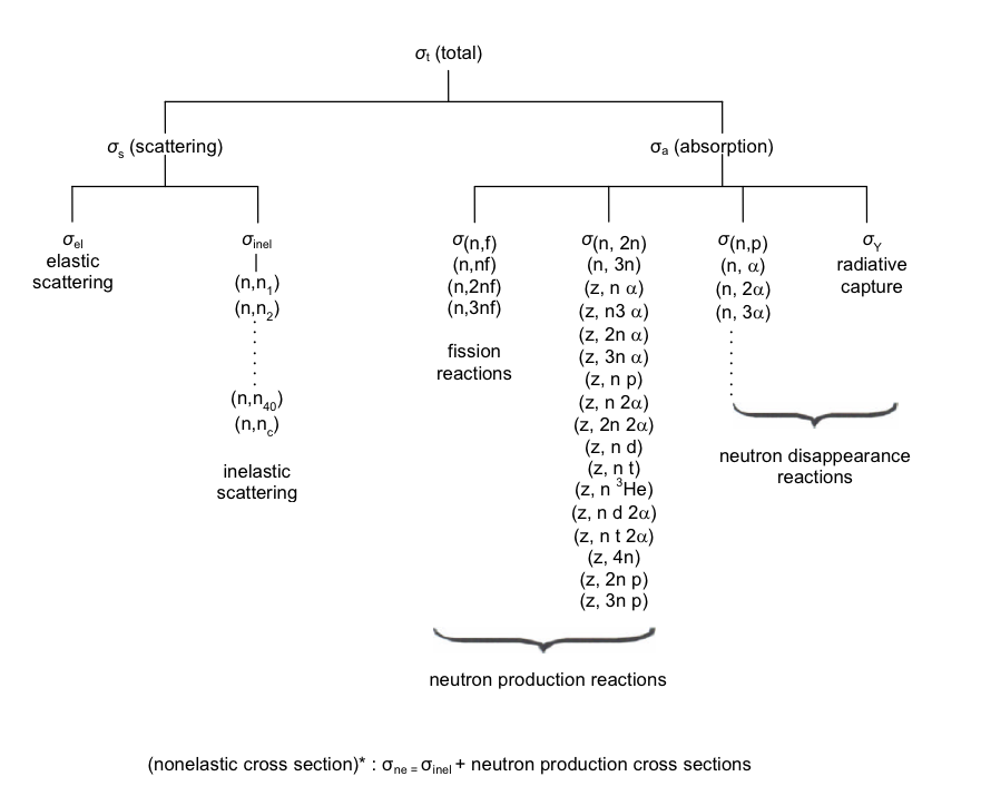
Fig. 8.1.204 Cross section hierarchy for particle interactions.

2. Select the exiting angle for the collision. The cross section library provides a kinematics data block that provides the angle and energy distributions of secondary particles for a specified reaction. Each record for each section of a reaction provides a flag (NPU) indicating the number of secondary angles for that energy. If the NPU flag is 1 and the corresponding cosine value is -2 (set as a programming flag), then the reaction is isotropic. The exiting angle for the collision can be obtained as follows:

   1. Isotropic Emission

   If the LAND flag is 0 for the secondary angular distribution, the exiting angle cosine is sampled uniformly between -1 and +1:

   (8.1.25)\[\mu = 2R - 1\]

   If the LAND flag is 1 for the secondary angular distribution, the exiting angle cosine must be sampled from an anisotropic distribution provided in the cross section library for the specified reaction. Details for sampling the exiting angle from the angular distribution data are provided in Sect. 8.1.7.2.6.

   The secondary angular distribution data are provided as a function of incident energy. The initial record of each section for a reaction provides the number of incident energies (NE) for the secondary angular and energy distributions. Corresponding to each incident energy is a secondary angular distribution. Therefore, there will be NE records used to describe the secondary angular data for each section.

   For each angular distribution record, there is an LMU flag and a NPU flag that describes the format of the data. The LMU flag designates whether the secondary distribution is provided in equiprobable cosine bins or in nonequiprobable cosine bins. The procedures for sampling the two types of data are provided in Sect. 8.1.7.2.7. The LMU flag must be the same for all NE records within a section. The NPU flag specifies the number of cosine values in the distribution.

   Based on the incident energy of the neutron, the angular distribution data are sampled according to the procedures of Sect. 8.1.7.2.7 to obtain the exiting angle cosine, \(\mu\), in the lab system.

3. Select the exiting energy for the collision. In addition to the angular distributions of the kinematics data, the cross section library provides the energy distributions of secondary particles for a specified reaction.

   The secondary energy distributions are provided as a function of incident energy and secondary angle cosine in each section. Once the exiting angle cosine is selected, the exiting energy is selected from the energy distribution that corresponds to the (E, \(\mu\)) pair. The exit energy is determined using the procedures of Sect. 8.1.7.2.7.

   For each energy distribution record, there is an LE flag and an NPE flag describing the format of the data. The LE flag designates whether the secondary distribution is provided in equiprobable energy bins or in nonequiprobable energy bins. The procedures for sampling the two types of data are provided in Sect. 8.1.7.2.7. Note that the LE flag must be the same for all NE records within a section for the secondary energy distribution data. The NPE flag specifies the number of secondary energy values in the distribution. For elastic scattering and discrete-level inelastic scattering, the NPE flag will equal the NPU flag due to the one-to-one correspondence between angle and energy.

4. Select the azimuthal angle \(\eta\) uniformly between 0. and \(2 \pi\) (i.e., \(\eta=2 R \pi\).

5. Calculate the new direction cosines in the lab system using the following equations:

   (8.1.26)\[u^{'} = u\mu - \sqrt{\nu^{2}+w^{2}} \sqrt{1-\mu^{2}}\text{cos}(\eta)\]
   (8.1.27)\[\nu^{'} = \nu \mu + \frac{u\nu}{\sqrt{\nu^{2}+w^{2}}}\text{cos}(\eta)\sqrt{1-\mu^{2}} - \frac{w}{\sqrt{\nu^{2}+w^{2}}}\sqrt{1-\mu^{2}}\text{sin}(\eta)\]
   (8.1.28)\[w^{'} = w\mu + \frac{uw}{\sqrt{\nu^{2}+w^{2}}}\text{cos}(\eta)\sqrt{1-\mu^{2}} + \frac{v}{\sqrt{\nu^{2}+w^{2}}}\sqrt{1-\mu^{2}}\text{sin}(\eta)\]

   where

   u, \(\nu\), and w = initial direction cosines,

   \(u^{\prime}, \nu^{\prime}, \text { and } w^{\prime}\) = exiting direction cosines,

   \(\mu\) = cosine of the scattering angle, and

   \(\eta\) = cosine of the azimuthal angle.

8.1.7.2.5. Fission treatment

As noted in the previous section, an implicit approach is used to treat a fission event. During the collision treatment, the fission weight is calculated using Eq. (8.1.23). After processing the collision, the fission weight is evaluated to determine if the fission treatment should be applied. If the fission weight is greater than zero, the collision occurred in fissile material. During the random walk, several fission source points must be generated to provide an adequate representation of the true source distribution. A minimum production factor is defined at the beginning of each generation to ensure that enough fission points are generated:

(8.1.29)\[mpf = \frac{3.0\bar{k}}{\sqrt{FG}} ,\]

where

\(\bar{k}\) = running average of \(k_{eff}\) through the current generation, and

FG = number of histories per generation.

Eq. (8.1.29) represents an estimate of the 99% lower confidence interval for the distribution of the generation k-effective.

If the fission weight is greater than zero, a pseudo-fission weight is calculated as follows:

(8.1.30)\[pfw = \frac{w_{f}}{R} = \frac{\nu^{-i}(E)\sigma^{i}_{f}(E)}{R\sigma^{i}_{t}(E)}w_{b} .\]

If the pseudo-fission weight is less than the minimum production factor given by Eq. (8.1.29) fission points are not generated and tracking of the particle continues. However, if the pseudo-fission weight is greater than the minimum production factor, pfw is redefined to be the minimum production factor divided by a random number:

(8.1.31)\[pfw = \frac{mpf}{R}\]

Once the pseudo-fission weight is redefined, a fission point can be generated. Each time a fission point is generated, the pseudo-fission weight is stored with the point in the fission bank. When a new point is stored in the fission bank, the energy and angular cosine must be selected from the kinematics data. Once the kinematics data are sampled for the new fission point, the fission weight of the history is decremented by the minimum production factor. If the remaining fission weight is greater than zero, the fission treatment procedures are repeated until the fission weight of the history has been exhausted (i.e., \(w_f \leq 0\)).

8.1.7.2.6. Sampling details

The preceding sections describe the procedures for the continuous energy random walk for KENO. During the random walk, KENO must sample various tables of data that may include probability tables and angle-energy distributions for secondary particles.

8.1.7.2.6.1. Probability tables

For each isotope with unresolved resonance data, multiple probability tables may be used to describe the URR. The header block for each isotope has an LPTAB flag that provides the number of probability tables for an isotope. Each table is defined for a range of incident energies between \(E_i\) and \(E_{i+1}\), and the energy range for a table should not overlap with another table for the isotope. For a particle with energy E, a search must be performed to find the probability table with energy bounds that bracket the particle energy, \(E_{i} \leq E < E_{i+1}\). Once the appropriate table is identified, the table can be sampled to obtain the total, elastic scattering, fission and capture cross section values in the URR.

The probability table block provides four separate records that correspond to each reaction within a table; however, the probability table construction is based on the total cross section. Therefore, the probabilities in each table refer to the total cross section band values, and the bands should be sampled based on the total cross section. Once the band is sampled, the corresponding partial reaction cross section values are selected from the same band as the total cross section. The cross section format permits the probability table to be expressed in equiprobable or nonequiprobable cross section bands (i.e., LBND = 0 or 1, respectively). The procedures for sampling both types of tables are provided in the subsequent subsections.

8.1.7.2.6.2. Equiprobable cross section bands

Each probability record has an NB parameter that designates the number of cross section bands for a table. If the table is constructed with equiprobable cross section bands, the k^th band can be selected as follows:

(8.1.32)\[k = NB \ ^{\ast} R + 1\]

where

R = random number [0., 1).

Based on the sampled cross section band, the total cross section corresponding to k^th band is extracted from the table. Likewise, the elastic scattering, fission and capture cross section values that correspond to the k^th band are also extracted from their respective records in the probability-table block.

8.1.7.2.6.3. Nonequiprobable cross section bands

If the LBND flag is 1, the cross section bands in the table are not equiprobable, and a different procedure must be used to sample the appropriate cross section band. For this case, the probability values in the table must be constructed as a cumulative distribution function. As noted previously, each probability record has an NB parameter that designates the number of cross section bands for a table, and the k^th band can be selected as follows:

(8.1.33)\[\sum^{k-1}_{j=1}P_{j} < R\sum^{NB}_{j=1}P_{j} \leq \sum^{k}_{j=1}P_{j} ,\]

where

P\(j\) = probability corresponding to the j^th cross section band.

Based on the sampled cross section band, the total cross section corresponding to the k^th band is extracted from the table. Likewise, the elastic scattering, fission and capture cross section values that correspond to the k^th band are also extracted from their respective records in the probability-table block.

8.1.7.2.7. Kinematics data

The kinematics data in the KENO library are provided in the lab or target-at-rest system as opposed to the center-of-mass system. By adhering to the lab coordinate system, KENO does not have to transform between different coordinate systems during the random walk; however, the energy and angle representations for elastic and discrete-level inelastic scattering become more complex in the lab system. For example, an angular distribution that is isotropic in the center-of-mass system is anisotropic in the lab system. Moreover, the secondary energy distribution as a function of exit angle in the lab system can be double valued (i.e., two possible exit energies with respect to a single angle) for energies above the threshold for the reaction. Likewise, a similar double valued distribution is observed for elastic scattering with hydrogen in the lab system if the actual mass ratio is used (i.e., A = 0.99928 as opposed to A = 1.0). Consequently, special care must be exercised in the construction of the secondary angle and energy distributions in the lab system.

The subsequent sections address the general procedures for sampling the kinematics data with emphasis on the special cases that must be addressed during the random walk. In Sect. 8.1.7.2.7.1, the general procedures for sampling the kinematics data are provided, Sect. 8.1.7.2.7.4 discusses isotropic angular data with energy coupling, while Sect. 8.1.7.2.7.5 discusses coherent and incoherent elastic scattering. A discussion is also provided in Sect. 8.1.7.2.7.6 to describe the elastic and discrete-level inelastic treatment.

8.1.7.2.7.1. General procedures

The kinematics data format is designed to accommodate coupled angle energy distributions of secondary particles. The following discussion provides the procedures for sampling the coupled distributions. Special cases such as elastic and discrete level inelastic scattering are discussed after the “General Procedures” section.

The sampling procedures in the following sections assume that the angle and energy distributions are continuous in nature. As a result, interpolation procedures can be used to obtain intermediate angle or energy values between the tabulated angle or energy values. During the course of KENO development, there may be a need to provide an average angle or energy value for a bin. The kinematics format can be modified as needed to accommodate additional angle and energy representations. Therefore, the following procedures represent the anticipated approach for sampling the current form of the kinematics data.

8.1.7.2.7.2. Exit angle cosine

The first record for each reaction provides the number of sections (NSECT) used to describe the kinematics for the reaction. Within each section, the first record defines the incident energy range for the section. After the first record for a section, the first block of data provides the secondary angular distributions for NE different incident energies within the energy range of the section. Consequently, there will be NE different angular distribution records in the secondary angle cosine block. The kinematics format permits the anisotropic angular distributions to be expressed in either equiprobable or nonequiprobable cosine bins (i.e., LMU = 0 or 1, respectively). Moreover, the formats permit the number of cosine bins to vary as a function of incident energy. In particular, each cosine distribution record can have NPU secondary angles that correspond to NPU - 1 cosine bins.

Equiprobable Cosine Bins. If the incident energy, E, is between E_i and E_i+1, the angle cosine is sampled in both tables, and the exit angle cosine is obtained by interpolating between the two tables. If the angular distribution is provided in equiprobable cosine bins, the a^th bin is selected from the i^th table as follows:

(8.1.34)\[a = (NPU_{i} - 1) \ ^{\ast} R_{1} + 1 = NA_{i} \ast R_{1} + 1 .\]

In Eq. (8.1.34) a denotes an integer quantity, and NA_i is the number of cosine bins for the i^th table. Using a similar procedure, the b^th bin is selected from the i+1^st table:

(8.1.35)\[b = NA_{i+1} \ ^{\ast} R_{1} + 1\]

As noted for the i^th table, b is an integer quantity in Eq. Eq. (8.1.35) and NA_i+1 is the number of cosine bins for the i+1^st table. Once the cosine bins are selected, the cosine of the exiting angle from the i^th and i+1^st tables is calculated with Eq. (8.1.36) and Eq. (8.1.37), respectively:

(8.1.36)\[{\dot{\mu}}_{i} = \mu_{ia} + \left( a - NA_{i}*R_{1} \right)\left( \mu_{ia + 1} - \mu_{ia} \right) ,\]

(8.1.37)\[{\dot{\mu}}_{i + 1} = \mu_{i + 1b} + \left( b - NA_{i + 1}*R_{1} \right)\left( \mu_{i + 1b + 1} - \mu_{i + 1b} \right) .\]

The exiting angle cosine is obtained by interpolating between i and i+1 based on the incident energy grid:

(8.1.38)\[\ \mu = {\dot{\mu}}_{i} + \left( \frac{E - E_{i}}{E_{i + 1} - E_{i}} \right)\left( {\dot{\mu}}_{i + 1} - {\dot{\mu}}_{i} \right).\]

Nonequiprobable Cosine Bins. If the angular distribution is in the form of nonequiprobable cosine bins, the a^th bin is selected from the cumulative distribution function for the i^th table:

(8.1.39)\[C_{ia - 1} < R_{1} \leq C_{ia}\ ,\]

where

C\(_{ia-1}\) = cumulative probability corresponding to the \(a-1^{st}\) cosine bin,

C\(_{ia}\) = cumulative probability corresponding to the \(a^{th}\) cosine bin,

Using a similar procedure, the b^th bin is selected from the i+1^st table:

(8.1.40)\[C_{i + 1b - 1} < R_{1} \leq C_{i + 1b}\ ,\]

where

\(C_{ib-1}\) = cumulative probability corresponding to the \(b - 1^{st}\) cosine bin,

\(C_{ib}\) = cumulative probability corresponding to the \(b^{th}\) cosine bin.

If the cosine bins are not equiprobable and the PDF is represented by a continuous distribution, the bins are selected so that linear interpolation can be performed in the PDF. Because the CDF is obtained by integrating the PDF, the interpolation procedure for the CDF has a quadratic form. The value for \({\dot{\mu}}_{i}\) is obtained with the following equation:

(8.1.41)\[{\dot{\mu}}_{i} = \mu_{ia} + \frac{\sqrt{P_{ia}^{2} + 2s_{i}(R_{1} - C_{ia - 1})} - P_{ia}}{s_{i}}\ ,\]

and

(8.1.42)\[s_{i} = \frac{P_{ia + 1} - P_{ia}}{\mu_{ia + 1} - \mu_{ia}}\ ,\]

where

\(P_{ia}\) = value of the PDF corresponding to the lower boundary of the \(a^{th}\) cosine bin in the distribution for \(E_{i}\), and

\(P_{ia+1}\) = value of the PDF corresponding to the upper boundary of the \(a^{th}\) cosine bin in the distribution for \(E_{i}\).

Likewise, the equation for \({\dot{\mu}}_{i + 1}\) is obtained using an equation that is similar to Eq. (8.1.41)

(8.1.43)\[{\dot{\mu}}_{i + 1} = \mu_{i + 1b} + \frac{\sqrt{P_{i + 1b}^{2} + 2s_{i + 1}(R_{1} - C_{i + 1b - 1})} - P_{i + 1b}}{s_{i + 1}},\]

and

(8.1.44)\[s_{i + 1} = \frac{P_{i + 1b + 1} - P_{i + 1b}}{\mu_{i + 1b + 1} - \mu_{i + 1b}} ,\]

where

\(P_{i + 1b}\) = value of the PDF corresponding to the lower value of the \(b^{th}\) cosine bin in the distribution for \(E_{i+1}\), and

\(P_{i + 1b + 1}\) = value of the PDF corresponding to the upper value of the \(b^{th}\) cosine bin in the distribution for \(E_{i+1}\).

The exiting angle cosine is obtained by interpolating between \({\dot{\mu}}_{i}\) and \({\dot{\mu}}_{i + 1}\) based on the incident energy using Eq. (8.1.38).

8.1.7.2.7.3. Exit energy

In the kinematics data block, each incident energy has a secondary distribution of NPU angle cosines. Therefore, there are NPU (E, \(\mu\)) pairs associated with each incident energy. For each (E, \(\mu\)) pair, there is a corresponding exit energy distribution that can have NPE exit energies. Because the kinematics data are tabulated in a coupled angle-energy format, the exit energy is obtained by a 2-D interpolation as shown in Fig. 8.1.205.

The objective of the sampling procedure is to sample the exit energy E’ in conjunction with the sampled angle cosine. Therefore, the interpolation for the exit energy is performed with an equation that is analogous to Eq. (8.1.38):

(8.1.45)\[E^{'} = E^{'}_{i} + \bigg(\frac{E - E_{i}}{E_{i+1} - E_{i}}\bigg) (E^{'}_{i + 1} - E^{'}_{i})\]

Based on Eq. (8.1.45), the values of \(E^{\prime}_{i}\) and \(E^{\prime}{ }_{i+1}\) must be obtained in order to calculate the exit energy for the collision. The a^th and b^th cosine bins are selected according to the procedures in Sect. 8.1.7.2.7.1 from tables i and i+1, respectively. As a result, the secondary energy distributions corresponding to the a^th and b^th cosine bins must be used to sample the exit energies from tables i and i+1. The details for sampling the energy bins are deferred for the moment. Once the appropriate energy bins are sampled from the two tables, the interpolation for \(E^{'}_{i}\) and \({E_{i+1}}\) is obtained with the following equations:

(8.1.46)\[E_{i}^{'} = E_{ia}^{'} + \left( \frac{{\dot{\mu}}_{i} - \mu_{ia}}{\mu_{ia + 1} - \mu_{ia}} \right)\left( E_{ia + 1}^{'} - E^{'}_{ia} \right)\ ,\]

(8.1.47)\[E_{i + 1}^{'} = E_{i + 1b}^{'} + \left( \frac{{\dot{\mu}}_{i + 1} - \mu_{i + 1b}}{\mu_{i + 1b + 1} - \mu_{i + 1b}} \right)\left( E_{i + 1b + 1}^{'} - E_{i + 1b}^{'} \right) .\]

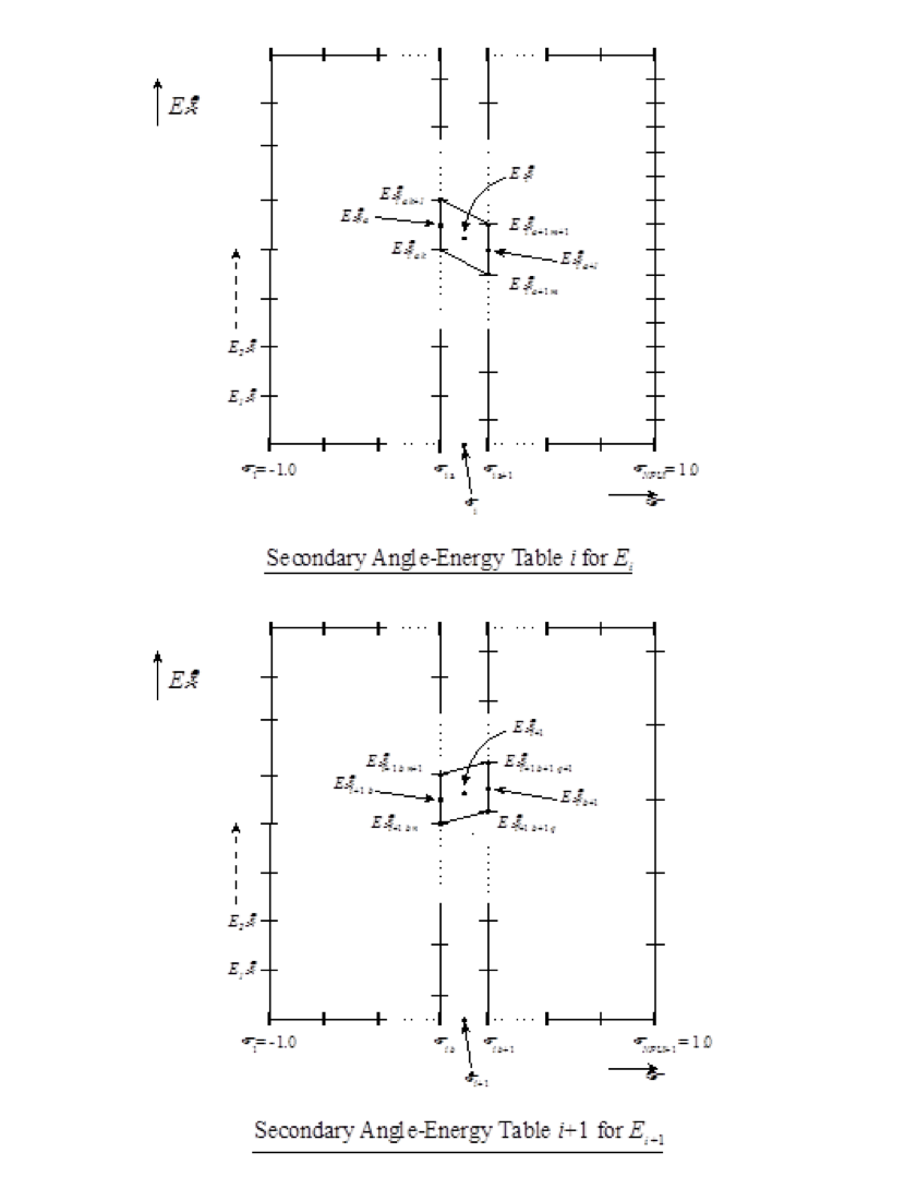
Fig. 8.1.205 Interpolation diagram for secondary angle-energy data.

Based on Eq. (8.1.46) and Eq. (8.1.47) the values for \(E^{'}_{ia}\), \(E^{'}_{ia + 1}\), and \(E^{'}_{ia + 1 b+1}\) and \(E^{'}_{i+1}\). The values for \(E^{'}_{ia}\) and \(E^{'}_{ia + 1}\) correspond to secondary energies that are coupled with the a^th and \(a+1^{st}\) angle cosines in Table i. Likewise, the values for \(E^{'}_{i+1 b}\) \(E^{'}_{i+1 b+1}\) correspond to the secondary energies that are coupled with the b^th and \(b+1^{st}\) angle cosines in Table i+1. Therefore, the exit energies from Table i are sampled from the secondary energy distributions that correspond to \(\left(E, \mu_{i a}\right)\) and \(\left(E, \mu_{i a+1}\right)\), and the energies from Table i+1 are sampled from the energy distributions for \(\left(E, \mu_{i+1} b\right)\) and \(\left(E, \mu_{i+1 b+1}\right)\).

As with the angular data, the secondary energy distributions may be provided in equiprobable or nonequiprobable energy bins. The following discussion provides the procedures for sampling the different distributions.

Equiprobable Energy Bins. In Table i, the k^th and m^th energy bins are sampled from the energy distributions for (E, \(\mu_{i \ a}\)) and (E, \(\mu_{i \ a+1}\)), respectively. The number of energy bins in a distribution is one less than the number of energies in the table (i.e., NPE - 1). If the energy distributions are provided in equiprobable bins, the k^th and m^th bins are selected as follows:

(8.1.48)\[k = (NPE_{ia} - 1)\ast R_{2} + 1 ,\]

(8.1.49)\[m = (NPE_{ia+1} - 1)\ast R_{2} + 1 .\]

The exiting energy values for \(E^{'}_{i \ a}\) \(E^{'}_{i \ a+1}\) are interpolated as follows:

(8.1.50)\[E^{'}_{ia} = E^{'}_{iak} + \bigg[k - (NPE_{ia} - 1)\ast R_{2}\bigg] \bigg(E^{'}_{iak+1} - E^{'}_{iak}\bigg) ,\]

(8.1.51)\[E^{'}_{ia+1} = E^{'}_{ia + 1m} + \bigg[m - (NPE_{ia+1} - 1)\ast R_{2}\bigg] \bigg(E^{'}_{ia+1m+1} - E^{'}_{ia+1m}\bigg) .\]

In Table i+1, the n^th and q^th energy bins are sampled from the energy distributions for \(\left(E, \mu_{i} b\right)\) and \(\left(E, \mu_{i b+1}\right)\), respectively. As presented for the i^th table, the n^th and q^th bins are selected from an equiprobable distribution in a manner analogous with Eq. (8.1.48) and Eq. (8.1.49):

(8.1.52)\[n = (NPE_{i+1b} - 1)\ast R_{2} + 1 ,\]

(8.1.53)\[q = (NPE_{i+1b+1} - 1)\ast R_{2} + 1 .\]

The exiting energy values for \(E_{i+1 \ b}\) and \(E_{i+1 b+1}\) are interpolated as follows:

(8.1.54)\[E^{'}_{i+1b} = E^{'}_{i+1bn} + \bigg[n - (NPE_{i+1b} - 1)\ast R_{2}\bigg] \bigg(E^{'}_{i+1bn+1} - E^{'}_{i+1bn}\bigg) ,\]

(8.1.55)\[E^{'}_{i+1b+1} = E^{'}_{i+1b+1q} + \bigg[q - (NPE_{i+1b+1} - 1)\ast R_{2}\bigg] \bigg(E^{'}_{i+1b+1q+1} - E^{'}_{i+1b+1q}\bigg) .\]

The exit energy from the i^th table (i.e., \(E^{'}\)) is obtained by substituting the values for \(E^{'}_{ia}\) and \(E^{'}_{ia+1}\) into Eq. (8.1.46), and the exit energy from the i+1^st table (i.e., \(E^{'}_{i+1}\)) is calculated by substituting the values for \(E^{'}_{ib}\) and \(E^{'}_{ib+1}\) into Eq. (8.1.47). Finally, the exit energy for the collision is obtained by inserting the calculated values for \(E^{'}_{i}\) and \(E^{'}_{i+1}\) into Eq. (8.1.45).

Nonequiprobable Energy Bins. If the energy distributions are provided in nonequiprobable bins, the k^th and m^th bins are sampled according to the cumulative distribution values:

(8.1.56)\[C_{iak - 1} < R_2 \leq C_{iak} ,\]

(8.1.57)\[C_{ia + 1m - 1} < R_2 \leq C_{ia+1m} ,\]

where

\(C_{iak - 1}\) = cumulative probability corresponding to the k-1^st energy bin in the \(\left(E, \mu_{i a}\right)\) distribution,

\(C_{iak}\) = cumulative probability corresponding to the k^th energy bin in the \(\left(E, \mu_{i a}\right)\) distribution,

\(C_{ia + 1m - 1}\) = cumulative probability corresponding to the m-1^st energy bin in the \(\left(E, \mu_{i} a+1\right)\) distribution, and

\(C_{ia+1m}\) = cumulative probability corresponding to the m^th energy bin in the \(\left(E, \mu_{i a+1}\right)\) distribution.

For the nonequiprobable bins, the bins for the secondary energy are selected so that linear interpolation can be performed in the PDF. Since the CDF is obtained by integrating the PDF, the interpolation procedure for the CDF is quadratic in form. As a result, the value for \(E^{'}_{i \ a}\) is obtained with the following equation:

(8.1.58)\[E^{'}_{ia} = E^{'}_{iak} + \frac{\sqrt{P^{2}_{iak} + 2s_{ia}(R_{2}-C_{iak-1})} - P_{iak}}{s_{ia}} ,\]

and

(8.1.59)\[s_{ia} = \frac{\sqrt{P_{iak+1} - P_{iak}}}{E^{'}_{iak+1} - E^{'}_{iak}} ,\]

where

\(P_{iak}\) = value of the PDF corresponding to the lower boundary of the k^th energy bin in the (E, \(\mu_{i \ a}\)) distribution, and

\(P_{iak+1}\) = value of the PDF corresponding to the upper boundary of the k^th energy bin in the (E, \(\mu_{i \ a}\)) distribution.

Likewise, the value for \(E_{i \ a+1}\) is obtained with the following equation:

(8.1.60)\[E^{'}_{ia+1} = E^{'}_{ia+1m} + \frac{\sqrt{P^{2}_{ia+1m} + 2s_{ia+1}(R_{2} - C_{ia+1m-1})} - P_{ia+1m}}{s_{ia+1}} ,\]

and

(8.1.61)\[s_{ia+1} = \frac{P_{ia+1m+1} - P_{ia+1m}}{E^{'}_{ia+1m+1} - E^{'}_{ia+1m}}\]

where

\(P_{ia+1m}\) = value of the PDF corresponding to the lower boundary of the m^th energy bin in the (E, \(\mu_{i a+1}\)) distribution, and

\(P_{ia+1m+1}\) = value of the PDF corresponding to the upper boundary of the m^th energy bin in the (E, \(\mu_{i a+1}\)) distribution.

For nonequiprobable distributions in the i+1^st table, the n^th and q^th bins are sampled according to the cumulative distribution values:

(8.1.62)\[C_{i+1bn-1} < R_{2} \leq C_{i+1bn} ,\]

(8.1.63)\[C_{i+1b+1q-1} < R_{2} \leq C_{i+1b+1q} ,\]

where

\(C_{i+1bn-1}\) = cumulative probability corresponding to the n-1^st energy bin in the (E, \(\mu_{i+1 \ b}\)) distribution,

\(C_{i+1bn}\) = cumulative probability corresponding to the n^th energy bin in the (E, \(\mu_{i+1 \ b}\)) distribution,

\(C_{i+1b+1q-1}\) = cumulative probability corresponding to the q-1^st energy bin in the (E, \(\mu_{i+1 \ b+1}\)) distribution, and

\(C_{i+1b+1q}\) = cumulative probability corresponding to the q^th energy bin in the (E, \(\mu_{i+1 \ b+1}\)) distribution.

As observed for the i^th table, the interpolation procedure for the CDF is quadratic in form, and the value for \(E^{'}_{i+1 \ b}\) is obtained as follows:

(8.1.64)\[E^{'}_{i+1b} = E^{'}_{i+1bn} + \frac{\sqrt{P^{2}_{i+1bn} + 2s_{i+1b}(R_{2} - C_{i+1bn-1})} - P_{i+1bn}} {s_{i+1b}} ,\]

and

(8.1.65)\[s_{i+1b} = \frac{P_{i+1bn+1} - P_{i+1bn}}{E^{'}_{i+1bn+1} - E^{'}_{i+1bn}} ,\]

where

\(P_{i+1bn}\) = value of the PDF corresponding to the lower boundary of the n^th energy bin in the (E, \(\mu_{i+1 b}\)) distribution, and

\(P_{i+1bn+1}\) = value of the PDF corresponding to the upper boundary of the n^th energy bin in the (E, \(\mu_{i+1 b}\)) distribution.

Likewise, the value for \(E^{'}_{i+1 b+1}\) is obtained with the following equation:

(8.1.66)\[E^{'}_{i+1b+1} = E^{'}_{i+1b+1q} + \frac{\sqrt{P^{2}_{i+1b+1q} + 2s_{i+1b+1}(R_{2} - C_{i+1b+1q-1})} - P_{i+1b+1q}}{s_{i+1b+1}} ,\]

and

(8.1.67)\[s_{i+1b+1} = \frac{P_{i+1b+1q+1} - P_{i+1b+1q}}{E^{'}_{i+1b+1q+1} - E^{'}_{i+1b+1q}} ,\]

where

\(P_{i+1b+1q}\) = value of the PDF corresponding to the lower boundary of the q^th energy bin in the (E, \(\mu_{i+1 b+1}\)) distribution, and

\(P_{i+1b+1q+1}\) = value of the PDF corresponding to the upper boundary of the q^th energy bin in the (E, \(\mu_{i+1 b+1}\)) distribution.

To obtain the exit energy for the collision, the energy from the i^th table (i.e., \(E^{'}_{i}\)) is calculated by substituting the values for \(E^{'}_{ia}\) and \(E^{'}_{ia+1}\) into Eq. (8.1.46), and the exit energy from the i+1^st table (i.e., \(E^{'}_{i+1}\)) is calculated by substituting the values for \(E^{'}_{ib}\) and \(E^{'}_{ib+1}\) into Eq. (8.1.47). Finally, the exit energy for the collision is obtained by inserting the calculated values for \(E^{'}_{i}\) and \(E^{'}_{i+1}\) into Eq. (8.1.45).

8.1.7.2.7.4. Isotropic Angular Distributions With Energy Coupling

The kinematics format can accommodate isotropic angular distributions in the coupled angle energy format. The following discussion describes the special case with the appropriate sampling procedures. If the secondary angular distribution is isotropic at an incident energy E, a single exit cosine with a value of -2.0 is specified in the (E, \(\mu\)) block. Therefore, the exit angle cosine is sampled uniformly between -1.0 and 1.0:

(8.1.68)\[\mu = 2R_{1} - 1 .\]

Because there is only one exit cosine specified in the (E, \(\mu\)) block, there is a single energy distribution record specified for the (E, \(\mu\)) pair. The general structure (i.e., material identifiers and data flags are omitted for clarity) of the kinematics data within a section for a reaction is presented in Table 8.1.30. As a result, the sampling procedure for the exit energy is based on the incident energy.

Table 8.1.30 Kinematics data structure for isotropic angular distributions

Once the angle is sampled according to Eq. (8.1.68), the exit energy is sampled in a manner that is analogous to the procedures of Sect. 8.1.7.2.7.3. If the incident energy, E, is between E_i and E_i+1, the k^th energy bin is sampled from the distribution corresponding to E_i using Eq. (8.1.69) or Eq. (8.1.70) for equiprobable or nonequiprobable distributions, respectively.

(8.1.69)\[k = \big(NPE_{i} - 1\big)\ast R_{2} + 1 ,\]

or

(8.1.70)\[C_{ik-1} < R_{2} \leq C_{ik} ,\]

where

\(NPE_{i}\) = number of exit energies corresponding to \(E_{i}\),

\(C_{ik-1}\) = cumulative probability corresponding to the k-1^st energy bin in the distribution for \(E_{i}\), and

\(C_{ik}\) = cumulative probability corresponding to the k^th energy bin in the distribution for \(E_{i}\).

For equiprobable energy bins, the exit energy corresponding to \(E_{i}\) is calculated as follows:

(8.1.71)\[E^{'}_i = E^{'}_{ik} + \bigg[k - \big(NPE_{i} - 1\big)\ast R_{2}\bigg] \bigg(E^{'}_{ik+1} - E^{'}_{ik} \bigg) .\]

If the secondary energy distributions are provided in nonequiprobable bins the exit energy is calculated using the following equation:

(8.1.72)\[E^{'}_{i} = E^{'}_{ik} + \frac{P^{2}_{ik} +2s_{i}\big(R_{2}-C_{ik-1}\big) - P_{ik}}{s_{i}} ,\]

and

(8.1.73)\[s_{i} = \frac{P_{ik+1} - P_{ik}}{E^{'}_{ik+1} - E^{'}_{ik}} ,\]

where

\(P_{ik}\) = value of the PDF corresponding to the lower boundary of the k^th energy bin in the distribution for \(E_{i}\), and

\(P_{ik+1}\) = value of the PDF corresponding to the upper boundary of the k^th energy bin in the distribution for \(E_{i}\).

By replacing i with i+1 in Eq. (8.1.69) through Eq. (8.1.73), the exit energy \(E^{'}_{i+1}\) can be calculated from the secondary energy distribution corresponding to the incident energy \(E_{i+1}\). Subsequently, Eq. (8.1.45) can be used to calculate the exit energy.

8.1.7.2.7.5. Coherent and incoherent elastic scattering

If thermal scattering law data are available for a material, the elastic scattering mechanism may be specified as either coherent or incoherent elastic scattering. Consequently, there is no change in energy resulting from either collision. The secondary energy distribution block for each (E, \(\mu\)) pair only has one exit energy with a value equal to the incident energy E. Therefore, the procedure for coherent or incoherent elastic scattering reduces to sampling the exit angle cosine. The procedures detailed in Sect. 8.1.7.2.7.2 are used to sample the exit angle cosine. The general structure of the kinematics data within a section for coherent or incoherent elastic scattering is presented in Table 8.1.31 with the material identifiers and data flags omitted for clarity. Once the angle cosine is selected, the exit energy is set equal to the incident energy.

Table 8.1.31 Kinematics data structure for coherent and incoherent elastic scattering

8.1.7.2.7.6. Elastic and discrete-level inelastic scattering

There is a one-to-one correspondence between the exiting angle and energy for elastic and discrete level inelastic scattering . Once the exiting angle is selected, the exiting energy is already determined based on the kinematics equations documented in most conventional reactor theory text books. However, an obscure fact is that the exiting energy distributions for discrete-level inelastic reactions and hydrogen elastic scattering can be double valued in the lab system. For discrete level inelastic scattering in the lab system, the range of incident energies that can have a double valued exit energy is given by the following expression:

(8.1.74)\[\Delta E_{double} = \frac{Q}{A(1-A)} ,\]

where

Q = the excess of the kinetic energy of the product particles over that of the original particles, and

A = atomic mass ratio of the target mass to the mass of a neutron.

Eq. (8.1.74) provides the size in energy of the double valued region above the threshold energy for the reaction. As indicated by Eq. (8.1.74), the range of energies for a double valued region is inversely proportional to the target mass. Using Eq. (8.1.74) and ENDF/B data, the values of \(\Delta E_{\text {double }}\) can be calculated for all discrete level inelastic scattering reactions for all isotopes. A plot of \(\Delta E_{\text {double }}\) as a function of atomic mass ratio is provided in Fig. 8.1.206 for all possible discrete level inelastic scattering collisions for all isotopes. As shown in Fig. Fig. 8.1.206, the size of the double valued region approaches 1 MeV as the mass ratio decreases. Because \(\Delta E_{\text {double }}\) can be relatively large, the double valued anomaly cannot be ignored in the collision treatment. The following discussion outlines the properties of the kinematics data and the procedures for treating elastic and discrete level inelastic scattering.

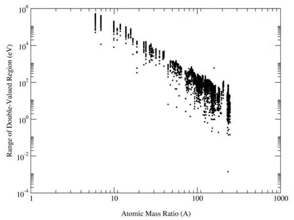
Fig. 8.1.206 Range of incident energies (\(\Delta\)E_double) for double valued region as a function of mass ratio.

As noted previously, NPU secondary angle cosines are provided for each incident energy for a reaction, and the cosine distribution can be represented with either equiprobable or nonequiprobable distributions. Depending on the type of distribution, procedures similar to those of Sect. 8.1.7.2.7.3 are used to sample an equiprobable or nonequiprobable angular distribution for the exit cosine in the lab system.

The angular data blocks for discrete level inelastic scattering and hydrogen elastic scattering are similar in form to other reactions; however, the exit lab cosines for discrete level inelastic scattering are greater than zero in the double-valued region, and an exit lab cosine may appear twice in the distribution with different probabilities. As an example, discrete level inelastic scattering for ⁷Li is characterized by a double valued exit energy distribution as a function of exit cosine in the lab system. Fig. 8.1.200 provides the exit energy distribution for an inelastic collision that leaves the ⁷Li nucleus in the first excited state (i.e., MT = 51) in the lab system. For ⁷Li, the threshold for MT = 51 is 5.4672 \(\times\) 10⁵ eV, and the double valued region extends from the threshold energy up to 5.58259 \(\times\) 10⁵ eV; therefore, the incident energy range of the double valued region is ~1.15 \(\times\)10⁴ eV. As shown in Fig. 8.1.200, the exit energy distributions are provided for different incident energies within the double valued region and an incident energy above the double valued region. As the incident energy exceeds the maximum energy for which two exiting energies can be produced, the secondary energy distribution becomes single valued (i.e., one exit energy for an exit cosine).

Note that the double valued anomaly does not occur in the center-of-mass system. Therefore, the two exit energies possible for the lab system actually correspond to two different center-of-mass exit cosines. During the preparation of the KENO library, the angular distribution tables for discrete level inelastic scattering and elastic scattering for hydrogen can be constructed in the center-of-mass system and subsequently converted to the lab system. In order to properly construct the angular distribution tables in the lab system, the minimum lab cosine, \(\mu\)^min_lab, must be determined because exit angles below the minimum lab cosine are not possible.

For discrete level inelastic scattering and elastic scattering, the exit cosine in the lab system can be expressed as a function of the center-of-mass scattering angle, \(\mu\)_cm:

(8.1.75)\[\mu = \frac{\gamma + \mu_{cm}}{\big(1+2\gamma\mu_{cm}+\gamma^{2}\big)^{1/2}} ,\]

where

(8.1.76)\[\frac{1}{\gamma} = \bigg[A^{2} + \frac{A\big(A+1\big)Q}{E}\bigg]^{1/2}\]

Physically, the quantity 1/\(\gamma\) represents the ratio of the exit velocity of the neutron in the lab system to the center-of-mass velocity. Moreover, the quantity 1/\(\gamma\) reduces to A for elastic scattering (i.e., Q = 0). The minimum value for \(\mu\) can be obtained by taking the derivative of Eq. (8.1.77) with respect to \(\mu\)_cm which yields the following expression:

(8.1.77)\[\frac{d\mu}{d\mu_{cm}} = \frac{1+ \gamma\mu_{cm}}{\big(1+2\gamma\mu_{cm}+\gamma^{2}\big)^{3/2}} .\]

Setting Eq. (8.1.77) equal to 0 reveals that the minimum lab cosine (\(\mu\)^min_lab) occurs when \(\mu\)_cm = -1/\(\gamma\). For elastic scattering, the minimum lab cosine occurs when \(\mu\)_cm = -A. Because hydrogen is the only nuclide with a mass ratio below 1, hydrogen is the only nuclide that has a double valued exit energy distribution in the lab system for elastic scattering.

During the preparation of the KENO library, the lab distributions for discrete level inelastic scattering and hydrogen elastic scattering will be constructed so that \(\mu\)^min_lab is a boundary for an angular bin, and no angular cosines in the lab system will be permitted below \(\mu\)^min_lab. As shown in Fig. 8.1.207 for ⁷Li, the exit cosines greater than \(\mu\)^min_lab will have two possible exit energies in the double valued region. As a result, the angular distribution table in the library will have angles that appear twice with different probabilities. For example, an angle cosine \(\mu\) may be present in the table with probabilities P_m and P_n. Although the value of the angle cosine is the same for both probabilities, the corresponding exit energy will be different for each (\(\mu\), P) pair. In other words, the probability for an exit cosine determines the location in the exit energy distribution table for selecting the outgoing energy.

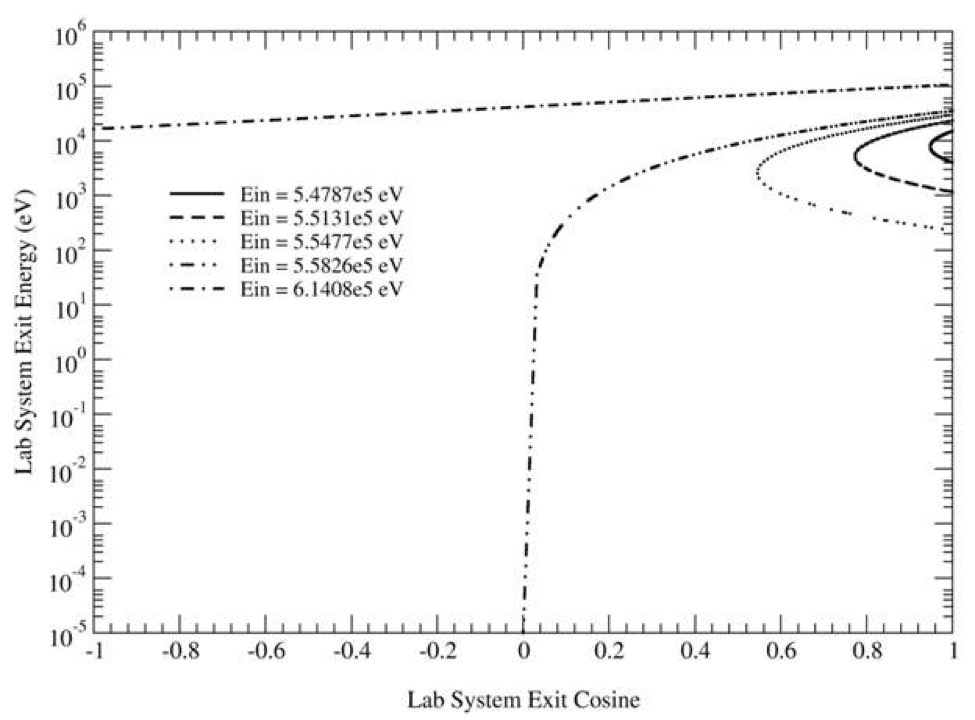
Fig. 8.1.207 ⁷Li exit energy distribution for the first discrete level inelastic scattering reaction (MT=51). E_threshold = 5.4672 \(\times\) 10⁵ eV; \(\Delta\)E_double = 1.1539 \(\times\) 10⁴ eV.

Based on the format of the kinematics data, angle cosine distributions are provided as a function of incident energy. If the incident energy, E, is between E_i and E_i+1, then the i^th table is selected with probability P_i and the i+1 table is selected with probability P_i+1:

(8.1.78)\[P_{i} = \frac{E_{i+1} - E}{E_{i+1}-E_{i}} ,\]

(8.1.79)\[P_{i+1} = \frac{E - E_{i}}{E_{i+1} - E_{i}} .\]

Once the angular distribution corresponding to the incident energy is selected, the exit angle cosine can be selected using procedures like those in Sect. 8.1.7.2.7.2 For example, if the i^th incident energy is selected, either Eq. (8.1.34)  is used to select the a^th cosine bin for equiprobable bins, or Eq. (8.1.39) is used for nonequiprobable bins. Subsequently, either Eq. (8.1.36) or Eq. (8.1.41) is used to calculate the exit angle cosine, depending on the type of angular distribution provided.

The coupled secondary angle-energy data blocks (E, \(\mu\), E’ ) follow the angular data block in the kinematics data. For elastic scattering and discrete level inelastic scattering, there is one possible exit energy. Therefore, in the exit energy distribution block, a single exit energy (NPE = 1) is provided for each (E, \(\mu\)) pair, and the general structure (i.e., material identifiers and data flags are omitted for clarity) of the secondary energy distribution data block is presented in Table 8.1.32. Because only one exit energy is provided for each (E, \(\mu\)) pair, the probability for the exit energy is 1.0. As indicated in Table 8.1.32, a cumulative probability of 1.0 is stored for each exit energy; however, the parameters stored in the PDF location are the power-interpolation parameters needed to interpolate the exit energy.

Table 8.1.32 Secondary energy distribution format for elastic and discrete-level inelastic scattering

When an exiting angle \({\dot{\mu}}_{i}\) is sampled between \(\mu\)_a and \(\mu\)_a+1, the exiting energy values that correspond to \(\mu\)_a and \(\mu\)_a+1 for the incident energy E_i can be used to interpolate the exiting energy E’ that corresponds to\({\dot{\mu}}_{i}\). Physically, the interpolation procedures correspond to an interpolation along one of the incident energy curves as depicted in Fig. 8.1.205. In order to perform the interpolation, the a^th and a+1^st (E, \(\mu\)) pairs are located in the secondary energy distribution block corresponding to E_i. Subsequently, the corresponding a^th and a+1 exit energy values (i.e., \(E^{'}_a\) and \(E^{'}_{a+1}\)) are read from the secondary energy distribution record.

The exiting energy is interpolated with the following relation:

(8.1.80)\[E^{'}\left( {\dot{\mu}}_{i} \right) = E_{a}^{'} + \left( \frac{{\dot{\mu}}_{i}^{P_{a}} - \mu_{a}^{P_{a}}}{\mu_{a + 1}^{P_{a}} - \mu_{a}^{P_{a}}} \right)\left( E_{a + 1}^{'} - E_{a}^{'} \right)\ ,\]

where

P = is a “power-interpolation” factor for the a^th cosine bin that is obtained from a fit to the E’ distribution as a function of \(\mu\).

The interpolation procedure in Eq. (8.1.80) is analogous to the interpolation scheme that has been used successfully to interpolate Bondarenko factors as a function of temperature in the BONAMI module. If the curve is monotonic in nature, the power-interpolation scheme can be used to represent the curvature with a minimum number of points. For elastic and discrete level inelastic scattering, the E’(\(\mu\)) distribution is monotonic and is suited for the power interpolation scheme. Note that if p is 1, Eq. (8.1.80) reduces to a linear interpolation in \(\mu\)-E’ space.

8.1.7.2.8. Thermal scattering effects

A collision between a neutron and nucleus can be affected by the thermal motion of the target nucleus. Moreover, ENDF provides thermal scattering law data to account for the thermal effects of scattering with a material below 10 eV; however, the scattering law data are only available for a select number materials as shown in Table 8.1.33. If thermal scattering law data are not available, elastic scattering is treated with the free gas approximation in the KENO library. For heavy nuclides with 0 K scattering libraries available, the Doppler Broadening Rejection Correction (DBRC) method is used instead. For DBRC-enabled nuclides, thermal scattering effects are taken into account up to 210 eV (although this parameter can be controlled by the user). More information on DBRC is given in Sect. 8.1.7.2.9.

Table 8.1.33 ENDF/B thermal scattering law data.

The continuous energy cross section library is processed to account for the appropriate scattering effects. As a result, the KENO cross section library inherently accounts for thermal scattering using either the thermal scattering law data or the free gas approximation. In other words, the kinematics data based on thermal effects are combined with the fast data to represent the collision kinematics for the material. As noted previously, the kinematics data block for a reaction is divided into sections that describe the collision kinematics for a range of incident energies. As a result, the kinematics data structure has a modular format that is beneficial for data library production. Because of the kinematics data structure, the thermal scattering law data, which are typically applied up to 10 eV, can be processed independently with AMPX to obtain the angle energy probability distributions. Subsequently, one or more sections in the kinematics data block can be used to represent the thermal angle -energy distributions for energies up to 10 eV. Moreover, the fast kinematics data can be represented with one or more sections for energies above 10 eV. As part of the library preparation, the thermal kinematics data are combined with the fast kinematics data block to complete the collision representation for the entire range of incident energies. Because the thermal scattering effects are treated during the processing of the cross section data for a material, the thermal effects are inherently treated in KENO. The 10 eV cutoff energy for thermal scattering can be input by the parameter THC in the parameter input. Using a cutoff value above 10 eV increases the energy range of free gas approximation because AMPX processed thermal scattering law data are available up to 10 eV, and this may increase the runtime in the sampling process while improving the accuracy in the results for some casees. During the Monte Carlo random walk, the procedures provided in Sect. 8.1.7.2.7.2 and Sect. 8.1.7.2.7.3 are used to sample the exit angle and energy for the collision.

8.1.7.2.9. Doppler broadening rejection correction method

When colliding with a heavy nuclide, the thermal motion of the target nuclide can significantly affect the exit angle and energy of the neutron. The thermal motion of the target nuclide was previously ignored, but this assumption has been proven inadequate by Dagan and Becker [BDL09].

A new sampling equation has been implemented to allow for Doppler broadening of the scattering kernel. Removing this approximation can have a significant impact on the critical eigenvalue of systems by allowing neutrons to be upscattered into absorption resonances. Currently, DBRC is enabled in KENO only for ²³⁸U, and this feature can be activated by setting the parameter DBR=1.

8.1.7.2.10. Doppler broadening methods

CE KENO calculations will perform temperature adjustment of neutron cross sections by default. The cross sections provided with SCALE are typically supplied in 300 K intervals, and additional cross section temperature resolution may be desired to model non-room temperature systems or systems with significant temperature effects.

The capability to perform problem-dependent Doppler broadening of nuclear cross sections has been implemented in KENO. This feature is controlled by the DBX parameter, which causes KENO to perform Doppler broadening on the cross sections in all compositions in a problem before simulating particle histories. When this occurs, the cross sections for each material are broadened to the temperature assigned to that material in the READ COMP block, as long as the requested temperature is more than 4 K from the library temperature. Within this \(\pm\) 4 K band, the library temperature is used to avoid difficulties with numerical instabilities in small cross section adjustments. The default for this feature is DBX=2, which performs Doppler broadening for both the 1-D and 2-D cross sections. Current options available are as follows:

• DBX = 0 – Doppler broadening is not performed. KENO selects the library at the closest temperature. If desired, the user can use the TTL parameter to force a job abort if the library temperature is too far from the requested temperature. By default, TTL=-1, so the closest library will be used regardless of the temperature difference.

• DBX=1 – Doppler broadening is performed using a finite difference method on the one-dimensional cross sections that are temperature dependent. Logarithmic interpolation is also used to broaden the probability table data. When this option is used, the collision probabilities are recalculated after the Doppler broadening is complete to ensure consistency.

• DBX=2 – The same actions as DBX=1 are performed, and Doppler broadening is also performed on the thermal moderator data by conducting interpolation on the double differential probability data present on the cross section library.

Nuclide level energy unionization is automatically disabled (M2U=NO) when Doppler broadening is enabled in order to reduce the memory usage. At this writing, research is in progress to allow KENO to perform on-the-fly cross section Doppler broadening as particle histories are being simulated.

8.1.7.3. Multigroup mode solution procedure

(8.1.81)\[\frac{1}{v_{g}}\frac{\partial\Phi_{g}}{\partial t}\left( X,\Omega,t \right) + \Omega \bullet \nabla\Phi_{g}\left( X,\Omega,t \right) + \Sigma_{\text{tg}}\left( X \right)\ \Phi_{g}\left( X,\Omega,t \right) = \mathrm{q}_{\mathrm{g}}\left( X,\Omega,t \right),\]

where

• \(g\) is the energy group of interest,

• \(v_g\) is the average velocity of the neutrons in group g,

• \(\Phi_g \left(X,\Omega,t \right)\) is the angular flux of neutrons having their energies in group g, at position X and time t, and

• \(\Sigma_{tg} \left( X \right)\) is the macroscopic total cross section of the media at position X for group g, corresponding to

(8.1.82)\[\Sigma_{tg}(X) = \frac{\int^{}_{\Delta E_{g}}\Sigma_{t}(X,E)\Phi(X,E,\Omega,t)dE} {\int^{}_{\Delta E_{g}}\Phi(X,E,\Omega,t)dE} ,\]

where

• \(\Delta E_g\) defines group g, and

• \(q_g \left(X,\Omega,t \right)\) is the total source contributing to energy group g at position X, and time t in direction \(\Omega\).

Using the relationship \(X^{\prime} = X - R\Omega\), defining the problem to be time independent using an integrating factor on both sides of Eq. (8.1.81), and defining

(8.1.83)\[T(R) = \int^{R}_{0}\Sigma_{tg}(X - R^{'}\Omega)dR^{'} ,\]

the following equation can be written:

(8.1.84)\[\Phi_{g}(X,\Omega) = \int^{\infty}_{O}q_{g}(X - R\Omega,\Omega)e^{-T(R)}dR .\]

At this point, the problem becomes an eigenvalue problem. If there is no external source, the source may be defined as

(8.1.85)\[q_{g}\left( X,\Omega \right) = \sum_{g^{'}}^{}{\int_{}^{}{{d\Omega^{'}}\Phi_{g^{'}}\left( X,\Omega^{'} \right)\ \Sigma_{s}\left( X,g^{'} \rightarrow g,\Omega^{'} \cdot \Omega \right)} + \frac{1}{k}Q_{g}^{'}\left( X,\Omega \right)},\]

where

• k is the largest eigenvalue of the integral equation,

• \(Q^{\prime}_{g}\left(X,\Omega \right)\) is the fission source at position X for energy group g and direction \(\Omega\) (all fission contributions to group g from all energy groups in the previous generation), and

• \(\Sigma_s \left(X,g^{\prime}\rightarrow g,\Omega^{\prime} \rightarrow \Omega \right)\) is the scattering cross section for scattering at position X from group \(g^{\prime}\) and direction \(\Omega^{\prime}\) to group g and direction \(\Omega\).

In terms of energy, the scatter can be defined as

(8.1.86)\[\Sigma_{s}\left( X,g^{'} \rightarrow g,\Omega^{'} \cdot \Omega \right) = \frac{\int_{\mathrm{\Delta}E_{g}}^{}{\int_{\mathrm{\Delta}E_{g^{'}}}^{}{\Sigma_{s}\left( X,E^{'} \rightarrow E,\Omega^{'} \cdot \Omega \right)\ \Phi\left(X,E^{'},\Omega^{'} \right)\text{d}E^{'}\text{dE}}}}{\int_{\mathrm{\Delta}E_{g^{'}}}^{}{\Phi\left( X,E^{'},\Omega^{'} \right)\text{dE}^{'}}\ }\ \ ,\]

where

\(\Delta E_g\) is the energy-range-defining energy group g, and

\(\Delta E_g'\) is the energy-range-defining energy group g’.

Assuming the fission neutrons to be isotropic, the fission source \(Q_{g^{\prime}}\left(X,\Omega \right)\) can be written as

(8.1.87)\[Q^{'}_{g}(X,\Omega) = \frac{1}{4\pi}\sum_{g^{'}}\int_{\Omega^{'}}^{}{d\Omega^{'}\Phi_{g^{'}}(X,\Omega^{'})\chi(X,g^{'}\rightarrow g)\nu_{g^{'}}(X)\Sigma_{fg^{'}}(X)} ,\]

where

• \(\chi \left(X,g^{\prime} \rightarrow g \right)\) is the fraction of neutrons born in energy group g from fission in energy group g in the media at position X,

• \(\nu_{g^{\prime}}\left(X \right)\) is the number of neutrons resulting from a fission in group \(g^{\prime}\) at position X, and

• \(\Sigma_{fg^{\prime}} \left( X \right)\) is the macroscopic fission cross section of the material at position X for a neutron in energy group \(g^{\prime}\).

Substituting Eq. (8.1.85) into Eq. (8.1.84) yields the following equation:

(8.1.88)\[\begin{split}\begin{gathered} \Phi_{g}(X, \Omega)=\int_{0}^{\infty} d R e^{-T(R)}\left\{\frac{1}{k} \mathrm{Q}_{g}^{\prime}(X-R \Omega, \Omega)\right. \\ \left.+\sum_{g^{\prime}}\left[\int_{\Omega^{\prime}} d \Omega^{\prime} \Phi_{g^{\prime}}\left(X-R \Omega, \Omega^{\prime}\right) \Sigma_{s}\left(X-R \Omega, g^{\prime} \rightarrow g, \Omega^{\prime} \cdot \Omega\right)\right]\right\} \end{gathered}\end{split}\]

The definition of k may be given as the ratio of the number of neutrons in the (n + 1)th generation to the number of neutrons in the nth generation or the largest eigenvalue of the integral equation. Using Eq. (8.1.87), Eq. (8.1.88) can be written as

(8.1.89)\[\begin{split}\begin{gathered} \Phi_{g}(X, \Omega)=\int_{0}^{\infty} d R e^{-T(R)}\left\{\sum_{g^{\prime}} \frac{1}{k} \int_{\Omega^{\prime}} v_{g^{\prime}}(X-R \Omega) \Sigma_{f g^{\prime}}(X-R \Omega) \chi\left(X-R \Omega, g^{\prime} \rightarrow g\right) \Phi_{g}\left(X-R \Omega, \Omega^{\prime}\right) \frac{d \Omega^{\prime}}{4 \pi}\right. \\ \left.+\sum_{g^{\prime}}\left[\int_{\Omega^{\prime}} d \Omega^{\prime} \Sigma_{t g^{\prime}}\left(X-R \Omega, \Omega^{\prime}\right) \Sigma_{s}\left(X-R \Omega, g^{\prime} \rightarrow g, \Omega^{\prime} \cdot \Omega\right)\right]\right\} \end{gathered}\end{split}\]

Writing Eq. (8.1.89) in generation notation, multiplying and dividing certain terms by \(\Sigma_{\mathrm{t}}(\mathrm{X})\), and multiplying both sides of the equation by \(\nu_{\mathrm{g}}(\mathrm{X}) \Sigma_{\mathrm{fg}}(\mathrm{X})\) yields the following equation, which is solved by KENO:

(8.1.90)\[\begin{split}\begin{gathered} \frac{v_{g}(X) \Sigma_{f g}(X)}{\Sigma_{t g}(X)} \Sigma_{t g}(X) \Phi_{g, n}(X, \Omega)=\frac{v_{g}(X) \Sigma_{f g}(X)}{\Sigma_{t g}(X)} \Sigma_{t g}(X) \int_{0}^{\infty} d R e^{-T(R)} \\ \left\{\frac{1}{k} \sum_{g^{\prime}}\left[\int_{\Omega^{\prime}} \frac{v_{g^{\prime}}(X-R \Omega) \Sigma_{f s^{\prime}}(X-R \Omega)}{\Sigma_{t g^{\prime}}(X-R \Omega)} \chi\left(X-R \Omega, g^{\prime} \rightarrow g\right) \Sigma_{t g^{\prime}}(X-R \Omega) \Phi_{g^{\prime}, n-1}\left(X-R \Omega, \Omega^{\prime}\right) \frac{d \Omega^{\prime}}{4 \pi}\right]\right. \\ \left.+\sum_{g^{\prime}}\left[\int_{\Omega^{\prime}} \frac{\sum_{s}\left(X-R \Omega, g^{\prime} \rightarrow g, \Omega^{\prime} \cdot \Omega\right)}{\Sigma_{t g^{\prime}}(X-R \Omega)} \Sigma_{t g^{\prime}}(X-R \Omega) \Phi_{g^{\prime}, n}\left(X-R \Omega, \Omega^{\prime}\right) d \Omega^{\prime}\right]\right\} \end{gathered}\end{split}\]

where n indicates the nth generation and n - 1 is the (n - 1)th generation. Note that the left-hand side of the equation — \(v_{\mathrm{g}}(\mathrm{X}) \sum_{\mathrm{fg}}(\mathrm{X}) \Phi_{\mathrm{g}, \mathrm{n}}(\mathrm{X}, \Omega)\) — is the fission production for the nth generation.

The solution strategy used by KENO solves Eq. (8.1.90) by using an iterative procedure. The fission production at point X in energy group g due to neutrons in the (n - 1)th generation, normalized to the system multiplication, is

(8.1.91)\[\frac{1}{k}\sum_{g^{'}}\int_{\Omega^{'}}\frac{\nu_{g^{'}}(X)\Sigma_{fg^{'}}(X)}{\Sigma_{tg^{'}}(X)}\chi \big(X,g^{'} \rightarrow g\big)\Sigma_{tg^{'}}\big(X\big)\Phi_{g^{'},n-1}\big(X,\Omega^{'}\big)\frac{d\Omega^{'}}{4\pi} .\]

The collision points used in KENO are chosen by selecting path lengths from the distribution

e^-T(R) ,

which is the probability of transport from any position X - R\(\Omega\) to position X.

The first collision density of neutrons in group g per unit solid angle about \(\Omega\) resulting from the fission source produced by the (n - 1) generation, normalized to the system multiplication, is

(8.1.92)\[\frac{\Sigma_{tg}\big(X\big)\int^{\infty}_{0}dRe^{-T(R)}\frac{1}{k}\int_{\Omega^{'}}\sum_{g^{'}}\frac{\nu_{g^{'}}\big(X-R\Omega\big)\Sigma_{fg^{'}}\big(X-R\Omega\big)}{E_{tg^{'}}\big(X-R\Omega\big)}}{\chi\big(X-R\Omega,g^{'}\rightarrow g\big)\Sigma_{tg^{'}}\big(X-R\Omega\big)\Phi_{g^{'},n-1}\big(X-R\Omega,\Omega^{'}\big)\frac{\text{d}\Omega^{'}}{4\pi}} .\]

The scattering source at position X emerging in group g and direction \(\Omega\) resulting from previous collisions in the same generation, is

(8.1.93)\[\sum_{g^{\prime}} \int_{\Omega^{\prime}} \frac{\Sigma_{s}\left(X, g^{\prime} \rightarrow g, \Omega^{\prime} \cdot \Omega\right)}{\Sigma_{t g^{\prime}}(X)} \Sigma_{t g}^{\prime}(X) \Phi_{g^{\prime}, n}(X, \Omega) d \Omega^{\prime}\]

The collision density in group g, per solid angle about \(\Omega\) is

(8.1.94)\[\Sigma_{t g} \int_{0}^{\infty} d R e^{-T(R)} \sum_{g^{\prime}} \int_{\Omega^{\prime}} \frac{\Sigma_{s}\left(X-R \Omega, g^{\prime} \rightarrow g, \Omega^{\prime} \cdot \Omega\right)}{\Sigma_{t g^{\prime}}(X-R \Omega)} \Sigma_{t g^{\prime}}(X-R \Omega) \Phi_{g^{\prime}, n}\left(X-R \Omega, \Omega^{\prime}\right) d \Omega^{\prime}\]

The total collision density times \(\frac{\nu_g(X)\Sigma_{fg}(X)}{\Sigma_{tg}(X)}\) is the relationship from which KENO picks the source points for the next generation.

8.1.7.3.1. Collision treatment in KENO

A collision occurs in a geometrical region when a history exhausts its mean-free-path length within the boundaries of the region. For each collision, the absorbed weight and the fission weight are tabulated, then the weight is modified by the nonabsorption probability. This new weight is checked for splitting and Russian roulette, and if it survives, the history is scattered. A new energy group is selected from the cumulative transfer probability distribution. This group-to-group transfer determines an angular scattering distribution, usually expressed as a Legendre expansion of the cross section transfer array. A set of discrete angles and probabilities are generated by a generalized Gaussian quadrature procedure, preserving the moments of the Legendre expansion of the angular scattering distribution. KENO treats P₀ and P₁ Legendre expansions as special cases. If the scattering distribution is isotropic, a flag is set to randomly select new direction cosines from an isotropic distribution, instead of using discrete scattering angles. If the distribution is a P₁ expansion, KENO randomly selects the cosine of the scattering angle according to

1. \(|\bar{\mu}| < \frac{10^{-10}}{3}\): scattering distribution is isotropic,

2. \(|\bar{\mu}| \leq 1/3: \mu = \bigg(\sqrt{1+6\zeta\bar{\mu}+\big(3\bar{\mu}\big)^{2}} - 1\bigg)/ 3\bar{\mu}\),

or

3. \(|\bar{\mu}| > 1/3: \mu = \zeta\big(1-|\bar{\mu}|\big) + \bar{\mu}\)

where \(\zeta\) is a uniform random variable between -1 and +1 and

\(\bar{\mu}\) is the mean cosine of the scattering angle.

Otherwise, KENO randomly selects one of the discrete scattering angles (\(\mu\)). New direction cosines are then calculated according to the following relationships where u, v, and w are the initial direction cosines and u’, v’, and w’ are the direction cosines after the collision:

u’ = ucos\(\Psi - \sqrt{\text{v}^{2} + \text{w}^{2}}\)sin\(\Psi\)cos\(\eta\)

v’ = vcos\(\Psi + \frac{\text{uv}}{\sqrt{\text{v}^{2} + \text{w}^{2}}}\text{cos}\eta\text{sin}\Psi - \frac{\text{w}}{\sqrt{\text{v}^{2} + \text{w}^{2}}}\text{sin}\Psi\text{sin}\eta\)

w’ = wcos\(\Psi + \frac{\text{uw}}{\sqrt{\text{v}^{2} + \text{w}^{2}}}\text{cos}\eta\text{sin}\Psi + \frac{\text{v}}{\sqrt{\text{v}^{2} + \text{w}^{2}}}\text{sin}\Psi\text{sin}\eta\)

where

\(\sin \psi\) = \(\sqrt{1-\mu^{2}}\),

\(\cos \psi\) = \(\mu\) = cosine of the scattering angle,

\(\eta\) = a random azimuthal angle between 0 and \(2 \pi\).

8.1.7.3.2. Fission point selection

In order for a fission to occur, a neutron must first have a collision. The fission weight, \(\text{fisw}\), is defined as the neutron weight, \(\text{wt}\), times the \(\nu\)-fission probability, \(\text{fnfp}\):

(8.1.95)\[fisw = wt\ \times \ fnfp\]

Two important variables used in the processing of fission points are (1) FWR, which is defined as the fission weight, \(\text{fisw}\), divided by a random number, and (2) RAKBAR, which is defined as a factor times the running average value of k-effective, AKBAR. This factor is a function of the square root of the number of neutrons per generation and was chosen because it usually produces an adequate number of independent fission points and does not produce so many that an excessive amount of time is spent choosing from the fission points produced.

The following procedure for generating fission points is repeated until FWR is less than RAKBAR. A fission point is generated only if FWR is greater than RAKBAR. Multiple fissions at the same point are allowed only if \(\text{fisw}\) is greater than RAKBAR. If \(\text{fisw}\) is greater than RAKBAR, a fission point is stored with FWR set equal to RAKBAR divided by a random number and \(\text{fisw}\) is decremented by RAKBAR. Then the energy group of fission is chosen randomly from the fission spectrum of the mixture in which the fission occurred. The energy group of fission, the X, Y, and Z position, the location of the unit within the array, the region number, the value of FWR, the region number of the array boundary, and the nesting data for holes and/or arrays are stored in the fission bank. The quantity of fission points kept to be used as fission positions for the next generation is limited to the number of positions in the fission bank (input parameter NFB=). Typically NFB is equal to the input parameter NPG, the number of neutrons per generation. If a fission occurs and the fission counter is less than NFB, the fission point information is stored in the fission bank. If a fission occurs and the fission counter is greater than or equal to the number per generation, a search is made to find the smallest stored value of FWR. If FWR of the newly fissioned neutron is less than the smallest FWR in the table, it is discarded. Otherwise, the information from the newly fissioned neutron replaces that associated with the smallest value of FWR found in the table.

When the next generation is ready to be processed, data are transferred from the fission bank into the neutron bank to be used as starting positions for the fission neutrons. If more than NPG neutrons are saved in the fission bank, NPG of those having the highest values of FWR will be used. If too few fission positions were stored (less than the number per generation), a warning message to that effect (K?-132) is printed, and additional fission points are randomly chosen from those that were stored until the number of fission points available to start the next generation is equal to the number of neutrons per generation.

8.1.7.3.3. Biasing or weighting

In order to minimize the statistical deviation of k-effective per unit computer time, KENO uses weighted tracking rather than analog tracking. Weighted tracking accounts for absorption by reducing the neutron weight rather than allowing the neutron history to be terminated by absorption. To prevent expending excessive computer time tracking low-weight neutrons, Russian roulette is played when the weight of the neutron drops below a preset weight, WTLOW. Neutrons that survive Russian roulette are assigned a weight, WTAVG. The value of WTLOW and WTAVG can be assigned as a function of position and energy. The values used by KENO are

DWTAV = 0.5, the default value of WTAVG,

WTAVG = DWTAV, the weight given a neutron that survives Russian roulette, and

WTLOW = WTAVG/3.0, the value of weight at which Russian roulette is played.

A study [Hof82] by Hoffman shows these default values to be reasonable for bare critical assemblies. Fig. 8.1.208 from this study shows the analytic relationship between the variance and WTLOW when WTAVG is 0.5. Note that the default value of 0.167 for WTLOW is very close to the minimum point on the curve. Experimental results of actual Monte Carlo calculations⁷ provide further assurance that 0.167 is an optimum choice for WTLOW when WTAVG is 0.5.

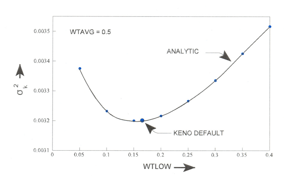
Fig. 8.1.208 Analytic estimate of the relationship between WTLOW and the variance, \(\sigma^{2}_{k}\), when WTAVG is 0.5.

Fig. 8.1.209, also from the Hoffman study, shows the analytic relationship between the variance and the value chosen for WTAVG for a value of WTLOW = 0.167. Although the KENO default value for WTAVG is not the optimum, a close examination of the data shows that the variance was changing relatively slowly as a function of WTAVG. Even though this study shows a value near 0.26 to be optimum for this system, further studies of other systems are needed before changing the default value of WTAVG from 0.5 as it has been used in previous versions of KENO.

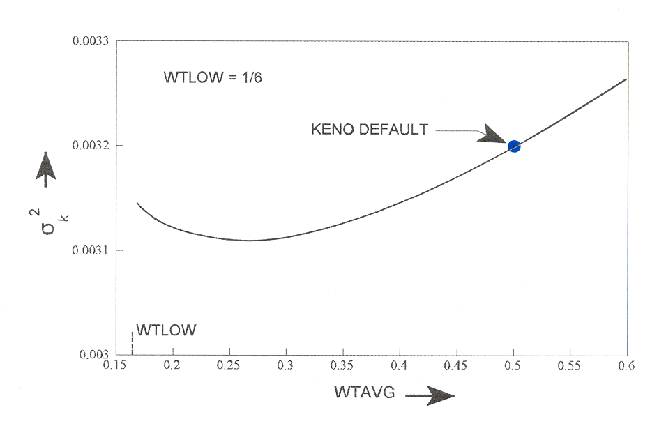
Fig. 8.1.209 Analytic estimate of the relationship between WTAVG and the variance, \(\sigma^{2}_{k}\), when WTLOW is ¹/₆.

Inside a fissile core, the importance of a neutron is a slowly varying function in terms of energy and position. Hence, for many systems, the standard defaults for WTLOW and WTAVG are good values to use. For reflectors, however, the worth of a neutron varies as a function of distance from the fissile material and as a function of energy. As a neutron in the reflector becomes less important relative to a neutron in the fissile region, it becomes desirable to spend less time tracking it. Therefore a space- and energy-dependent weighting or biasing function is used in KENO to allow the user to minimize the variance in k-effective per unit of tracking time. When a biasing function is used in a reflector, it becomes possible for a neutron to move from one importance region into another in which the WTLOW is greater than the weight of the neutron. When this occurs, Russian roulette is played to reduce the number of neutrons tracked. When the reverse occurs, that is, when the neutron moves to a region of higher importance, its weight may be much higher than WTAVG for that region. When the weight of the neutron is greater than a preset value, WTHI, the neutron is split into two neutrons, each having a weight equal to one-half the weight of the original neutron. This procedure is repeated until the weight of the split neutron is less than WTHI. The default value for WTHI is WTAVG*3.0. WTHI is the weight at which splitting occurs.

The weighting or biasing function for a given core material and reflector material can be obtained by using the adjoint solution from S_n type programs for a similar (usually simplified) problem. This adjoint flux gives the relative contribution of a neutron at a given energy and position to the total fissions in the system. The weighting function for KENO is thus proportional to the reciprocal of the adjoint flux. Although such a function can be difficult to obtain, the savings gained makes the effort worthwhile for many of the materials that are frequently used as reflectors. Biasing functions [ODellA87] have been prepared for several reflector materials commonly used in KENO calculations. The use of biasing to minimize the variance in k-effective per unit of computer time will usually increase the variance in other parameters such as leakage or absorption in the reflector.

8.1.7.3.4. Differential albedos

Arrays reflected by thick layers of material having a small absorption to the scattering ratio may require large amounts of computer time to determine k-effective[Dem99a] because of the relatively long time a history may spend in the reflector. A differential albedo technique was developed for use with the KENO codes to eliminate tracking in the reflector. This involves returning a history at the point it impinges on the reflector and selecting an emergent energy and polar angle from a joint density function dependent upon the incident energy and polar angle. The weight of the history is adjusted by the functional return from the reflector, which is also based on the incident energy and angle.

The characteristics of a differential albedo emulate the attributes of the reflector material and are independent of the material or materials adjacent to the reflector. Thus, a differential albedo that is generated for a given reflector material can be used with any array, regardless of the type of fuel or fissile material contained within the array.

For many calculations involving reflected arrays of fissile material, the differential albedo treatment is a powerful tool that can significantly reduce the computing time required to determine k-effective. The savings will vary depending on the importance of the reflector to the system. A substantial effort is required to generate a differential albedo, but the savings gained were well worth the effort for commonly used reflector materials. The savings are not worth the applicability questions on modern computing platforms; the differential albedo capability is maintained only for backwards compatibility.

To generate the differential albedo information for a material, a fixed-source calculation must be made for each incident energy and angle. The data presently available for use with KENO were generated by 1-D discrete ordinates calculations for slab geometry representing infinite slabs. Consequently, for a finite reflector, these data will not correctly treat histories that enter the reflector near an edge. Past experience with differential albedo reflectors indicates that k-effective appears to be conservative for small faces and will tend toward the correct result as the face becomes large relative to the area near the corners. Care must be taken to ensure that any surface to which a differential albedo is applied is large enough that the errors at the edges can be ignored.

Because differential albedos are expensive and time consuming to generate, those corresponding to the Hansen-Roach 16-energy-group structure are the only differential albedos available for use with KENO at this writing. In the past, their use was limited to problems using cross sections having the Hansen–Roach 16-energy-group structure. KENO extends the use of differential albedos to other energy-group structures by allowing appropriate energy transfers. This is accomplished by creating lethargy boundary tables for the albedo group structure and the cross section group structure and determining the lethargy interval corresponding to the desired transfer (cross section group structure to albedo group structure or vice versa) based on a uniform lethargy distribution over the interval. When the energy-group boundaries of the cross sections and albedos are different, the results should be scrutinized by the user to evaluate the effects of the approximations.

8.1.7.4. KENO Geometries

KENO V.a geometry is restricted to the use of specific shapes. These shapes are called geometry regions or regions. Allowed shapes in KENO V.a are cubes, cuboids (rectangular parallelepipeds), spheres, cylinders, hemispheres, and hemicylinders. These shapes must be oriented along orthogonal axes and cannot be rotated in KENO V.a. They can be translated. Hemispheres and hemicylinders are not limited to half spheres and half cylinders; the definitive plane can be positioned by entering a chord. The value of this chord can range from the positive magnitude of the radius (giving a complete sphere or cylinder) to the negative magnitude of the radius (giving a zero volume, nonexistent sphere or cylinder).

KENO-VI geometry can model any geometric shape that can be described using quadratic equations. These geometric shapes are stacked together forming regions. The set of regions is then used to build units. A set of predefined shapes that include cones, cuboids (rectangular parallelepipeds), cylinders, dodecahedrons, ecylinders (extruded elliptical cylinders), ellipsoids, hexprisms, hoppers, parallelepipeds, planes, rhombohedrons, spheres, wedges (triangular prisms), as well as others is used to construct regions. In addition, the keyword QUADRATIC is provided which allows additional shapes to be constructed by specifying the quadratic equations that describe the shape. These shapes can be rotated and translated to any orientation and position within their respective units. Hemispheres and hemicylinders can be constructed using spheres and cylinders with a chord. Regions are rotated by providing the nonzero angles associated with the Euler X-convention.

A major restriction applied to KENO V.a geometry is that intersections are not allowed. Furthermore, each successive geometry region must completely enclose the preceding region. Tangency and shared faces are allowed. The volume of a region is the volume of the specified shape minus the volume of the preceding region shape and any holes contained in the region. To alleviate the complete enclosure restriction, KENO V.a allows multiple sets of geometry regions, with each set independently governed by this restriction. Each set of these multiple geometry regions is called a unit. Units can be stacked together in a 3-D rectangular parallelepiped called an array or lattice, just as children’s blocks can be stacked. Units that are to be stacked together in this manner must have a rectangular parallelepiped outer region, and the adjacent faces of adjacent units must be the same size and shape. An array can be treated as a building block and used as a unit within another array.

A major improvement in KENO-VI is the ability to intersect regions. Region volumes are no longer calculated due to the complexity involved with intersecting regions. Each set of multiple geometry regions is called a unit. KENO-VI allows multiple sets of geometry regions (i.e., units), and each set has an independent coordinate system. A global unit must be specified for every problem, including single-unit problems. Units with cuboidal outer boundaries where the adjoining faces have the same dimensions can be stacked together in a 3-D rectangular parallelepiped called an array or lattice, just as children’s blocks can be stacked. Unlike KENO V.a, units having hexagonal or dodecahedral outer boundaries where the adjoining faces have the same dimensions can also be stacked together in an array. An array boundary must be specified that either coexists with the outermost edge of the array or that is entirely within the array. The array boundary can be any shape that is definable using quadratic equations. An array can be treated as a building block and used as a unit within another array.

The use of holes in KENO allows a unit to be emplaced within another unit. This feature allows the addition of a complex structure, previously defined as a unit, to be directly placed within another unit. In KENO V.a a hole is not allowed to intersect other holes or regions, but holes may intersect multiple regions in KENO-VI.

Multiple arrays can be described in KENO. The global array in an unreflected problem is the outermost array in the problem geometry description. The global array in a reflected problem is the array referenced by surrounding geometry regions following the last array placement description that does not immediately follow a unit number description. In KENO-VI, the outermost boundary is always specified as the global unit boundary. If the outermost boundary is to be the array boundary, a global unit must still be specified with the global unit boundary coinciding with the array boundary. Unlike past versions of KENO, KENO-VI cannot run a single unit problem without specifying a global unit.

8.1.7.5. Fluxes

Fluxes are computed in KENO with a track length estimator. The scalar flux in region z for energy group g for a single generation is computed as

(8.1.96)\[\Phi_{g,z} = \frac{\sum^{K}_{k=1}W_{k,z}l_{k,z}}{V_{z}\sum^{K}_{k=1}W_{k,0}} ,\]

where

l\(_{k,z}\) = distance traversed by particle k while within region z and energy group g,

W\(_{k,z}\) = weight of particle k while traversing region z,

V\(_z\) = volume of region z,

W\(_{k,0}\) = initial weight of particle k, and

K = total number of histories in the generation.

The average fluxes for all active generations and the standard deviation in the averages are also computed. Scalar fluxes computed by KENO are reported in units of neutrons per cm² per initial source neutron.

KENO is also capable of computing the angular flux for a level symmetric quadrature set. The angular flux for energy group g in region z for quadrature direction n is computed as

(8.1.97)\[\Phi^{n}_{g,z} = \frac{\sum_{k=1}^{K}W_{k,z}l_{k,z,n}}{V_{z}\sum^{K}_{k=1}W_{k,0}} ,\]

where

l_k,z,n = the distance traversed by particle k while within region z and energy group g within the quadrature direction n.

The angular flux can be expanded to flux moments using an appropriate spherical harmonics expansion. KENO has even number symmetric level quadrature sets S₂-S₁₆.

Flux moments can also be computed directly in KENO. The jth moment, which corresponds to real valued spherical harmonics functions [Dem99b] for a single generation for energy group g in region z, is computed as

(8.1.98)\[ \phi^{j}_{g,z} = \frac{\sum_{k=1}^{K}R^{j}_{k}W_{k,z}l_{k,z}}{V_{z}\sum^{K}_{k=1}W_{k,0}} ,\]

where

\(R^{j}_{k}\) = real valued spherical harmonics function for moment index j corresponding to the direction of particle k.

KENO offers the option of computing the angular fluxes and flux moments using a transformed coordinate system so that the moments are based on a polar rather than a Cartesian position vector. This is a 3-D extension of the 1-D method for calculating the flux moments in terms of Legendre polynomials based only on the direction cosine with respect to the spatial coordinate.

Here, \(\hat{i}\), \(\hat{j}\), and \(\hat{k}\) represent the directional coordinate system axes, \(\mu\), \(\eta\), \(\xi\) represent the direction cosines, and \(\theta\) and \(rho\)represent the polar and azimuthal angles of the “normal” coordinate system. The same symbols primed represent the transformed coordinate system. The transformed polar or \(\hat{k}^{'}\) axis is co-linear, with the position vector \(\vec{r}\) directed from the center of the region for which moments are desired to the point at which the flux tally occurs. By using the center of the region as a reference point, consistency of the moment calculation is assured with differing models of the same system. The \(\hat{i}^{'}\) and \(\hat{j}^{'}\) axes are chosen to form an orthogonal coordinate system, with \(\hat{i}^{'}\) held in the plane formed by \(\hat{i}\) and \(\hat{j}\). The use of constraints other than the restriction of \(\hat{i}^{'}\) to this plane may be explored in future studies. If an additional constraint is not placed on either \(\hat{i}^{'}\) or \(\hat{j}^{'}\), the transform would be able to rotate about \(\hat{k}^{'}\), and the consistency of consecutive transformations of the same direction could not be assured. With the transform computed, the position and direction of travel of the particle remain unchanged, but the quadrature directions and/or spherical harmonics terms are calculated using the transformed coordinate system. With the direction cosines consistently transformed for each history, the new polar and azimuthal angles can be computed and the spherical harmonics functions can be calculated for each history.

KENO offers a mesh flux tally in which the fluxes are computed in a user-defined cubic mesh superimposed on the geometry model. The mesh is defined from the origin of the global unit and is oriented with the Cartesian axes. At the end of each particle track, appropriate track lengths are assigned to the mesh intervals that were crossed for the region in which the track occurred. The length of the actual particle track is equal to the sum of the lengths assigned to the meshes encountered by the particle track. Because the coordinates of the mesh are defined in terms of the global unit, fluxes for regions in repeated units (i.e., units in arrays or holes) may be stored separately for each occurrence of the unit. The volumes of each region in each mesh interval are computed so that the fluxes are appropriately normalized on a per unit volume basis, consistent with Eq. (8.1.96). When the mesh flux option is activated, all requested fluxes, scalar, angular and/or moment, are computed for each mesh interval.

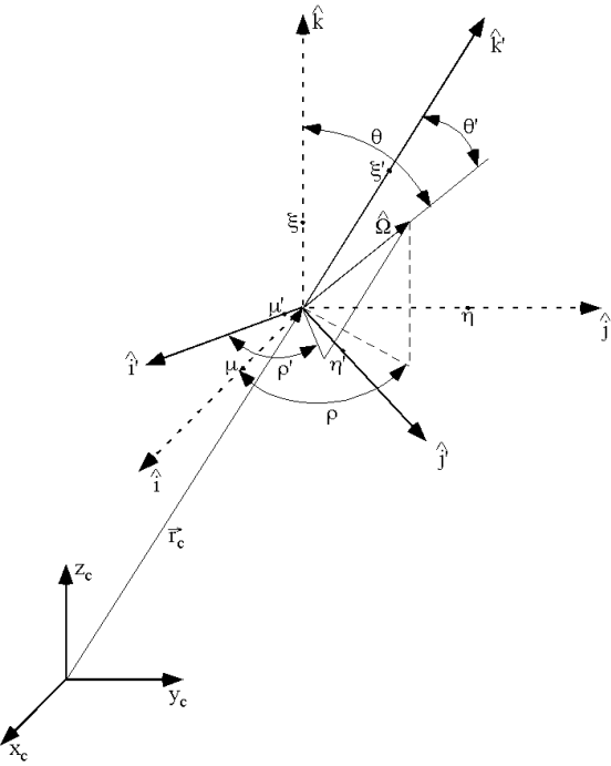
Fig. 8.1.210 Coordinate transform used for quadrature direction and spherical harmonics terms.

8.1.7.6. Reaction Rate and Few Group Micro Cross Section Calculations

A few-group microscopic reaction cross section calculation capability is included in the KENO codes to provide this data especially for the CE depletion calculations in SCALE. This new method produces multigroup cross sections and reaction rates directly in CE mode calculations rather than using a post-processing approach. In each generation, KENO uses track length estimators for the reaction rate tallies for all isotopes in each specified regions. At the end of each generation, a subsequent calculation is performed to compute few group microscopic reaction cross sections for all isotopes in a region as the ratio of the computed reaction rates to the flux averaged over this cell. Finally, KENO computes mean values and statistical uncertainties for all these quantities, and saves them in a file, which could be used by the depletion modules in SCALE.

Reaction tally calculations can be enabled by entering the required data in the reaction data block described in Sect. 8.1.3.15.

8.1.7.7. Source Convergence Diagnostics

Fission source convergence detection techniques are implemented in KENO to provide improved confidence in the computed k_eff and tally results. The dominance ratio of a system is equal to the ratio of the eigenvalue of the first nonfundamental mode to that of the fundamental mode, k₁/k₀. The dominance ratio is strongly related to the convergence rate of the fission source for systems, and problems with larger dominance ratios will require more inactive generations to produce reliable k_eff and reaction rate estimates. A converged k_eff estimate does not necessarily guarantee a converged fission source distribution, and the fission source and flux distribution may continue to evolve well after k_eff convergence is reached. Convergence of the fission source distribution is necessary to ensure that all regions containing fissile material in a model are adequately represented in the final k_eff estimate. Typically, the k_eff estimate converges much faster than the fission source and neutron flux distributions, and simulations may undersample important regions and produce inaccurate flux and reaction rate estimates if the user includes only enough inactive generations for the eigenvalue to converge. This is particularly important in models where one region is physically small but substantially more reactive than others (i.e. the k-effective of the World problem [Whi71]). The highly reactive region may not be adequately sampled, which may result in an underprediction of k_eff. Thus, it is essential to monitor the convergence of both the fission source distribution and k_eff; versions of KENO included in SCALE versions prior to SCALE 6.2 only monitored the convergence of k_eff, but diagnostic tools to identify unconverged fission source distributions are included in SCALE 6.2 and beyond.

Note

Due to limited experience with these tests in KENO, the Shannon entropy test results should be used as a supplement to guarantee that a problem’s fission source is converged. Failure of Shannon entropy tests typically indicates insufficient convergence of fission site source distributions. Whenever Shannon entropy tests report failure, users should review the plots of k_eff as a function of generation skipped and k_eff as a function of generation completed (Sect. 8.1.5.29 and Sect. 8.1.5.30) to ensure that the k_eff value is adequately converged. If it is not clear that the k_eff value is converged, users should rerun the calculation using a different number of neutrons per generation (using the NPG parameter) or using a different random number seed value (using the RND parameter) or a different starting source term distribution (using the READ START block).

It may also be possible to pass the Shannon entropy tests by changing the source convergence mesh (using the SCD parameter and the READ GRID block) or changing the number skipped generations (using the NSK parameter).

For KENO calculations that are used for other purposes (such as producing neutron flux and reaction rate distributions, fuel depletion calculations, or fission distributions for radiation transport calculations) in which the spatial dependence of the neutron flux and fission source may be more important, KENO calculations with failed Shannon entropy tests should be rerun because these spatially dependent distributions may not be adequately converged.

8.1.7.7.1. Shannon Entropy Statistics

The fission source distribution, S, is measured at the beginning of each generation using given spatial meshes. The state of source distribution at the j^th generation can then be characterized by Shannon entropy:

(8.1.99)\[H(S^{j}) = - \sum^{M}_{i}[S^{j}_{i}\text{log}_{2}(S^{j}_{i})] ,\]

where \({S}_{i}^{j}\) is the fraction of the fission source distribution from the j^th’ generation tallied in the spatial bin i, and M is the total number of spatial bins (typically represented using a spatial mesh). The value of H ranges from a maximum value of log₂M when the source distribution is uniform, and to a minimum value of zero when the whole source is located in a single bin. By computing H for each generation, the distribution of the fission source is used to generate a score for H for each generation, and the convergence of the fission source can be assessed by tracking the convergence and randomness of the values of H over each successive generation. Random fluctuations in the generation-to-generation Shannon entropy tallies make it difficult to determine if and when the Shannon entropy of a system has converged, so several metrics and tests are typically applied to examine the Shannon entropy and identify convergence in a system [Uek05].

The first test for fission source convergence is a comparison between the mean square of posterior relative entropy, and the centered mean square Shannon entropy. The posterior relative entropy, \(D(S^{j}\parallel T)\) , is defined as the statistical distance between the binned fission source \({S}^{j}_i\)and the average fission source over the second half of the active generations, T, and is given by

(8.1.100)\[D(S^{j}\parallel T) = \sum^{M}_{i}[S^{j}_{i}\text{log}_{2}(S^{j}_{i} / T_{i})] ,\]

where T is defined by

(8.1.101)\[T_{i} = \frac{2}{N}\sum^{N}_{j=N / 2+1}S^{j}_{i} ,\]

where N is the number of active generations. The posterior relative entropy is non-negative and becomes zero only when \({S}^{j}\)= T and achieves its maximum value when \(S^{j}\) is uniform.

The mean square posterior relative entropy is defined as

(8.1.102)\[msq(D) = \frac{2}{N}\sum^{N}_{j=N / 2+1}D(S^{j}_{i}\parallel T_{i})^{2} ,\]

and the centered mean square Shannon entropy is defined as

(8.1.103)\[cmsq(H) = \frac{2}{N-2}\sum^{N}_{j=N / 2+1}[H(S^{j}_{i}) - \bar{H}]^{2} ,\]

where \(\bar{H}\) is defined as

(8.1.104)\[\bar{H} = \frac{2}{N}\sum^{N}_{j=N / 2+1}H(S^{j}_{i}) .\]

This test compares the measure of fluctuations of Shannon entropy (cmsq(H)) with the measure of the magnitude of the penalty incurred by assuming T (msq(D)) and states that the fission source is converged if msq(D) < cmsq(H). This test is useful to determine whether the source is converged by the end of the calculation. Failure of this test indicates that the fission source was still moving during the active generations, which indicates that the number of skipped generations was not sufficient to converge the fission source.

The second test is given by

(8.1.105)\[D(S^{j}\parallel T) - [H(T-H(S^{j}))] \leq \varepsilon\]

where \(\mathcal{E}\) has been set to 0.1. This test verifies that the Shannon entropy of each active generation does not vary significantly from the average Shannon entropy of the system and should be valid over all active generations. For example, this test could detect an unconverged fission source for a problem with an undersampled, highly fissile fuel region, as any neutrons that reached this region would produce an outlier in the Shannon entropy tally for that generation. This test is especially useful for reporting the generation at which the source converged. Once the converged generation is determined, the user can repeat the calculation with the number of inactive generations (skipped generations) set to be the identified generation or greater to ensure that only contributions from generations with a converged source contribute to flux and reaction rate tallies. This test complements the first test since it will not be affected by whether or not the binned source is uniform.

The last test calculates whether

(8.1.106)\[H_{\eta} = H(S^{j}) - H_{b} \leq \eta ,\]

where H_b is the average Shannon Entropy over the second half of active generations, and \(\eta\) has been set to 0.1. This test verifies that the average Shannon entropy of all active generations does not differ significantly from the Shannon entropy of the last half of the active generations. This test is useful for detecting fission source convergence in problems where an inadequate number of inactive generations was sampled, as the Shannon entropy would continue to change during the active generations until it eventually converges.

8.1.7.7.2. Source Convergence Diagnostic Input

Because the processing of the source tallies for fission source convergence calculations is quite fast and produces small memory requirements, these source convergence diagnostics have been permanently enabled in KENO and require no additional input parameters. However, the KENO input specifications were updated to allow users to specify the spatial mesh data for the source convergence tests via the SCD parameter and READ GRID data block.

8.1.8. Appendices

• 8.1.8.1. KENO V.a Shape Descriptions
• 8.1.8.2. KENO VI Shape Descriptions
• 8.1.8.3. KENO Sample Problems
  • 8.1.8.3.1. CSAS-MG data
  • 8.1.8.3.2. KENO V.a sample problem data
    • 8.1.8.3.2.1. Sample Problem 1 2C8 BARE
    • 8.1.8.3.2.2. Sample Problem 2 CASE 2C8 BARE WITH 8 UNIT TYPES MATRIX CALCULATION
    • 8.1.8.3.2.3. Sample Problem 3 2C8 15.24-CM PARAFFIN REFL
    • 8.1.8.3.2.4. Sample Problem 4 2C8 15.24-CM PARAFFIN REFL AUTOMATIC REFL
    • 8.1.8.3.2.5. Sample Problem 5 2C8 12-INCH PARAFFIN ALBEDO REFLECTOR
    • 8.1.8.3.2.6. Sample Problem 6 ONE 2C8 UNIT (SINGLE UNIT)
    • 8.1.8.3.2.7. Sample Problem 7 BARE 2C8 USING SPECULAR REFLECTION
    • 8.1.8.3.2.8. Sample Problem 8 INFINITELY LONG CYLINDER FROM 2C8 UNIT
    • 8.1.8.3.2.9. Sample Problem 9 INFINITE ARRAY OF 2C8 UNITS
    • 8.1.8.3.2.10. Sample Problem 10 2C8 BARE WRITE RESTART
    • 8.1.8.3.2.11. Sample Problem 11 2C8 BARE READ RESTART DATA
    • 8.1.8.3.2.12. Sample Problem 12 4 AQUEOUS 4 METAL
    • 8.1.8.3.2.13. Sample Problem 13 TWO CUBOIDS IN A CYLINDRICAL ANNULUS
    • 8.1.8.3.2.14. Sample Problem 14 U METAL CYLINDER IN AN ANNULUS
    • 8.1.8.3.2.15. Sample Problem 15 SMALL WATER REFLECTED SPHERE ON PLEXIGLAS COLLAR
    • 8.1.8.3.2.16. Sample Problem 16 UO2F2 INFINITE SLAB K-INFINITY
    • 8.1.8.3.2.17. Sample Problem 17 93% UO2F2 SOLUTION SPHERE ADJOINT CALCULATION
    • 8.1.8.3.2.18. Sample Problem 18 1F27 DEMONSTRATION OF OPTIONS
    • 8.1.8.3.2.19. Sample Problem 19 4 AQUEOUS 4 METAL ARRAY OF ARRAYS (SAMP PROB 12)
    • 8.1.8.3.2.20. Sample Problem 20 TRIANGULAR PITCHED ARRAY
    • 8.1.8.3.2.21. Sample Problem 21 PARTIALLY FILLED SPHERE
    • 8.1.8.3.2.22. Sample Problem 22 CASE 2C8 BARE WITH 3 NESTED HOLES, EACH IS EQUAL VOLUME
    • 8.1.8.3.2.23. Sample Problem 23 CASE 2C8 BARE AS STACKED CYLINDERS
    • 8.1.8.3.2.24. Sample Problem 24 CASE 2C8 BARE AS STACKED ROTATED CYLINDERS
    • 8.1.8.3.2.25. Sample Problem 25 CASE 2C8 BARE AS MIXED YHEMICYLINDERS
    • 8.1.8.3.2.26. Sample Problem 26 (KENO V.a ONLY) CASE 2C8 BARE AS MIXED ZHEMICYLINDERS WITH ORIGINS
    • 8.1.8.3.2.27. Sample Problem 27 (KENO V.a oONLY) CASE 2C8 BARE AS MIXED XHEMICYLINDERS WITH ORIGINS
    • 8.1.8.3.2.28. Sample Problem 28 (KENO V.a oONLY) CASE 2C8 BARE AS MIXED YHEMICYLINDERS WITH ORIGINS
    • 8.1.8.3.2.29. Sample Problem 29 BARE CRITICAL SPHERE 3.4420-IN. RADIUS
    • 8.1.8.3.2.30. Sample Problem 30 (KENO V.a ONLY) BARE CRITICAL SPHERE Z HEMISPHERE MODEL 3.4420-IN. RADIUS
    • 8.1.8.3.2.31. Sample Problem 31 (KENO V.a ONLY) BARE CRITICAL SPHERE X HEMISPHERE MODEL 3.4420-IN. RADIUS
    • 8.1.8.3.2.32. Sample Problem 32 (KENO V.a ONLY) BARE CRITICAL SPHERE Y HEMISPHERE MODEL 3.4420-IN. RADIUS
    • 8.1.8.3.2.33. Sample Problem 33 CRITICAL TRIANGULAR PITCHED ARRAY OF ANNULAR RODS

References

BDL09

B. Becker, R. Dagan, and G. Lohnert. Proof and implementation of the stochastic formula for ideal gas, energy dependent scattering kernel. Annals of Nuclear Energy, 36(4):470–474, 2009. Publisher: Elsevier.

Dem99a(1,2)

L. Demaret. Accurate determination of confidence intervals in Monte Carlo eigenvalue calculations. In ICNC'99, Sixth Int. Conf. on Nuclear Criticality Safety, Versailles, France, Sep. 20-24. 1999, volume 1, 66–80. 1999.

Dem99b

L. Demaret. Accurate determination of confidence intervals in Monte Carlo eigenvalue calculations. In ICNC'99, Sixth Int. Conf. on Nuclear Criticality Safety, Versailles, France, Sep. 20-24. 1999, volume 1, 66–80. 1999.

DG02

M. E. Dunn and N. M. Greene. AMPX-2000: A Cross-Section Processing System for Generating Nuclear Data for Criticality Safety Applications. In Transactions of the American Nuclear Society, volume 86, 118–119. 2002.

Hof82

T. J. Hoffman. The Optimization of Russian Roulette Parameters for KENO Va. Technical Report ORNL/TM-7539, Union Carbide Corp., Nucl. Div., Oak Ridge National Laboratory, Oak Ridge, TN (USA), 1982.

ODellA87

R. Douglas O'Dell and Raymond E. Alcouffe. Transport calculations for nuclear analyses: Theory and guidelines for effective use of transport codes. Technical Report, Los Alamos National Laboratory, Los Alamos, NM (USA), 1987.

Tho64

J. T. Thomas. CRITICAL THREE-DIMENSIONAL ARRAYS OF NEUTRON-INTERACTING UNITS. PART II. U (93.2) METAL. Technical Report, Oak Ridge National Laboratory, Oak Ridge, TN (USA), 1964.

Tho73

Joseph T. Thomas. Critical three-dimensional arrays of U (93.2)-metal cylinders. Nuclear Science and Engineering, 52(3):350–359, 1973. Publisher: Taylor & Francis.

Uek05

Taro Ueki. Information theory and undersampling diagnostics for Monte Carlo simulation of nuclear criticality. Nuclear Science and Engineering, 151(3):283–292, 2005. Publisher: Taylor & Francis.

UMN97

Taro Ueki, Takamasa Mori, and Masayuki Nakagawa. Error estimations and their biases in Monte Carlo eigenvalue calculations. Nuclear science and engineering, 125(1):1–11, 1997. Publisher: Taylor & Francis.

Whi71

G. E. Whitesides. A Difficulty in Computing the k-effective of the World. In Transactions of the American Nuclear Society, volume 14, 680. 1971.