3.1. TRITON: A Multipurpose Transport, Depletion, And Sensitivity and Uncertainty Analysis Module

Code Responsible(s): F. Bostelmann Contributors: F. Bostelmann, K. Bekar, D. Wiarda, M. A. Jessee, U. Mertyurek, W. A. Wieselquist, S. W. Hart, S. E. Skutnik, B. R. Langley

The TRITON computer code is a multipurpose SCALE control sequence for transport, depletion, and sensitivity and uncertainty analysis. TRITON automates the processing of cross sections, the neutron transport calculations for one-, two-, and three-dimensional (1D, 2D, and 3D) configurations, and the depletion calculations to estimate the neutron flux, mixture-wise powers, isotopic concentrations, source terms, decay heat and other quantities as well as few-group homogenized cross sections for nodal core calculations as a function of burnup.

TRITON can be used in combination with any one of SCALE’s neutron transport kernels. Deterministic multigroup transport calculations for 1D and 2D geometries are performed using XSDRNPM and NEWT, respectively. The application of the Monte Carlo codes KENO V.a, KENO-VI, and Shift enables depletion calculations of 3D geometries in either multigroup or in continuous-energy mode. In MG mode, TRITON automates the preparation of problem-dependent MG cross sections for use in MG neutron transport calculations using SCALE’s cross section processing module XSProc. The depletion calculations are performed by the ORIGEN depletion module.

The SAMS module is used to determine the sensitivity of the calculated value of responses to the nuclear data used in the calculation as a function of nuclide, reaction type, and energy. The uncertainty in the calculated value of the response, resulting from uncertainties in the basic nuclear data used in the calculation, is estimated using energy-dependent cross section covariance matrices. The implicit effects of the cross section processing calculations are also treated.

3.1.1. Acknowledgments

The U.S. Nuclear Regulatory Commission (NRC) has been instrumental in supporting TRITON development and enhancements in each SCALE release. For SCALE 6.3 support, we express gratitude to M. Aissa (former NRC), D. Algama (former NRC), R. Y. Lee (former NRC), D. Barto, L. Kyriazidis, and H. Esmaili. Previous releases of SCALE-TRITON were funded by other government agencies and developed by several current and former ORNL staff. The original development of TRITON was led by Mark DeHart (former ORNL) who authored several sections in the current manual.

3.1.2. Introduction

TRITON (Transport Rigor Implemented with Time-dependent Operation for Neutronic depletion) is a multipurpose SCALE control sequence for transport and depletion analysis for reactor physics applications. By calling the appropriate SCALE modules, TRITON automates the processing of cross sections, the neutron transport calculations for one-, two-, and three-dimensional (1D, 2D, and 3D) configurations, and the depletion calculations to estimate the neutron flux, mixture-wise powers, isotopic concentrations, source terms, decay heat and other quantities as a function of burnup. An overview can be found in [TRITONDB11].

The choice of the neutron transport kernel determines whether TRITON is run in multi-group (MG) or in continuous-energy (CE) mode. TRITON can be used in combination with any one of SCALE’s neutron transport kernels. Deterministic MG transport calculations for 1D and 2D geometries are performed using XSDRNPM and NEWT, respectively. The application of the Monte Carlo codes KENO V.a, KENO-VI, and Shift enables depletion calculations of 3D geometries in either MG or in CE mode. In MG mode, TRITON automates the preparation of problem-dependent MG cross sections for use by the MG neutron transport kernels (see Fig. 3.1.1). Nodal data for use in nodal core simulations can be generated with the TRITON sequence that uses the NEWT deterministic transport code and with the TRITON sequences using the Shift Monte Carlo code.

Fig. 3.1.1 General flowchart of the TRITON reactor physics sequence.

The SAMS module is used to determine the sensitivity of the calculated value of the response to the nuclear data used in the calculation as a function of nuclide, reaction type, and energy. The uncertainty in the calculated value of the response, resulting from uncertainties in the basic nuclear data used in the calculation, is estimated using energy-dependent cross section covariance matrices. The implicit effects of the cross section processing calculations are predicted using SENLIB and BONAMIST.

As a SCALE control module, TRITON automates execution of SCALE functional modules and manages data transfer and input/output processes for multiple analysis sequences. Each of TRITON’s eleven calculational sequences is provided in Table 3.1.1, which lists the sequence name keyword, the sequence description, and the function modules invoked within each sequence. The method for cross section processing is selected using a separate “parm=” keyword, which is described in more detail in the next section.

Table 3.1.1 Overview of TRITON sequences.
Sequence keyword	Primary SCALE modules	parm= options	Sequence function
Cross section processing sequences
`=T-XSEC`	XSProc	bonami centrm^a xslevel=1/2/3/4	Preparation of multigroup (MG) cross section library.
Transport sequences
`=T-XSDRN`	XSProc, XSDRNPM	bonami centrm^a xslevel=1/2/3/4 weight^b	1D MG deterministic transport calculation.
`=T-NEWT`	XSProc, NEWT		2D MG deterministic transport calculation.
Depletion sequences
`=T-DEPL-1D`	XSProc, XSDRNPM, ORIGEN, OPUS	bonami centrm xslevel=1/2/3^a/4 addnux=0/1/2^a/3/4 weight^b	1D MG deterministic transport, coupled with ORIGEN depletion.
`=T-DEPL`	XSProc, NEWT, ORIGEN, OPUS		2D MG deterministic transport, coupled with ORIGEN depletion.
`=T5-DEPL`	XSProc^c KENO-V.a, ORIGEN, OPUS		3D, Monte Carlo transport (KENO-V.a), coupled with ORIGEN depletion.
`=T6-DEPL`	XSProc^c KENOVI, ORIGEN, OPUS		3D, Monte Carlo transport (KENO-VI), coupled with ORIGEN depletion.
`=T5-DEPL-SHIFT`	XSProc^c Shift, ORIGEN, OPUS		3D, Monte Carlo transport (Shift), coupled with ORIGEN depletion.
`=T6-DEPL-SHIFT`	XSProc^c Shift, ORIGEN, OPUS		3D, Monte Carlo transport (Shift), coupled with ORIGEN depletion.

^aDefault value. ^bparm=weight is used to generate a broad group cross section library. This parm option is only available for the T-DEPL sequence. ^cT5-DEPL and T6-DEPL are also available in CE-mode, which does not invoke XSProc for cross section processing.

3.1.2.1. TRITON Sequences

The TRITON control module supports eleven calculational sequences, each with its own design and applications. Each of these sequences is described in the following subsections.

The first subsection covers the basic cross section processing sequence T-XSEC. The T-XSEC sequence prepares problem-dependent multigroup cross sections for subsequent transport analysis. The second subsection covers TRITON’s transport analysis sequences, while the third subsection discusses TRITON’s depletion analysis sequences.

3.1.2.1.1. Cross section processing sequence (T-XSEC)

The T-XSEC sequence provides the ability to prepare a problem-dependent multigroup cross section library using SCALE cross section processing modules to appropriately account for spatial and energy self-shielding effects. The problem-dependent cross section library contains microscopic cross sections for each nuclide for each material composition defined in the TRITON input. SCALE provides several unit cell types (e.g., a lattice of pins, an infinite medium, a multiregion problem, or a doubly heterogeneous cell) to correct the cross sections for spatial and energy self-shielding. Multiple cell calculations can be used in the same calculation. The calculation of multigroup cross sections is executed by XSProc).

3.1.2.1.2. Transport sequences (T-XSDRN, T-NEWT)

The TRITON transport sequences build upon the cross section processing sequence by automating a transport calculation after cross section processing. Both 1D and 2D discrete-ordinates transport calculations can be performed using XSDRNPM and NEWT, respectively. The T-XSDRN sequence calls XSDRNPM for transport analysis in slab, sphere, or cylindrical geometries, while the T-NEWT sequence calls NEWT for analyses in 2D xy-geometries. In addition to the input necessary for cross section processing, an XSDRN or NEWT input model is also required. The XSDRN model input is discussed in Appendix A of TRITON; the NEWT model input requirements are described in the NEWT chapter. Similar capabilities and applications for KENO-V.a and KENO-VI are handled through the CSAS5 and CSAS6 sequences, respectively.

3.1.2.1.3. Depletion sequences (T-DEPL, T-DEPL-1D, T5-DEPL, T6-DEPL, T5-DEPL-SHIFT, T6-DEPL-SHIFT)

The TRITON depletion sequences build upon the transport sequences by automating depletion/decay calculations after the transport calculations for each material designated for depletion. One or more materials in the model can be designated for depletion. Each designated material is depleted using region-averaged reaction rates, accounting for all regions in the model associated with a given depletion material. The TRITON depletion calculation procedure is described further in the next subsection. TRITON automates the various computational processes-cross section processing, transport, and depletion-over a series of depletion and decay intervals supplied by the user. The depletion procedure is discussed in Sect. 3.1.2.2. The 2D TRITON depletion sequence (T-DEPL), which uses NEWT for the transport calculations and the 3D TRITON depletion sequences which use Shift in CE mode for the transport calculations (T5-DEPL-Shift, T6-DEPL-SHIFT) provide the capability to generate lattice-physics data for nodal core calculations.

Within TRITON depletion calculations, TRITON invokes the ORIGEN depletion module for the time-dependent transmutation of each user-defined material. TRITON provides ORIGEN the neutron flux space-energy distribution, the multigroup cross sections, material concentrations, and material volumes. ORIGEN performs the flux normalization, cross section collapse, and multi-material depletion/decay operations to determine new isotopic concentrations for the next calculation.

3.1.2.2. Predictor-corrector depletion process

For all depletion sequences, TRITON automates cross section processing, transport, and depletion calculations over a series of depletion-decay intervals supplied by the user. A depletion interval represents a time interval in which the model power level is assumed constant. A depletion model that exhibits various power level changes will require multiple depletion intervals to accurately model the changes in power. Each depletion interval can be followed by a decay calculation over a user-specified decay interval.

Within a given depletion interval (e.g., an LWR operating at constant power for a 12-month fuel cycle), the isotope concentrations of different depletion materials change, which induces changes in the problem-dependent multigroup cross sections (through spatial and energy self-shielding effects) as well as the neutron flux distribution, leading to different power distributions and transmutation rates in depletion materials. This requires TRITON to represent each depletion interval as a series of smaller time intervals in which cross section processing and transport solutions are recomputed to accurately model these time-dependent effects. A depletion subinterval represents a time interval in which TRITON performs cross section processing and transport calculations to determine cross sections and flux distributions used in the depletion calculations. All depletion subintervals for a given depletion interval have the same length-for example, one 12-month depletion interval can be represented as a series of 12 one-month depletion subintervals, or as 6 two-month depletion subintervals. Alternatively, the 12-month depletion interval can be modeled as two consecutive 6-month depletion intervals, each one having a different number of subintervals. Therefore the formulation of a depletion scheme in TRITON is highly flexible. A depletion scheme is the set of user-defined depletion and decay intervals with associated power levels and number of subintervals.

Caution

TRITON does not provide automated means to determine the appropriate depletion scheme for a given application. The user must determine the accurate depletion scheme specific to his or her application.

TRITON uses a predictor-corrector approach to process the user-defined depletion scheme. The predictor-corrector approach performs cross section processing and transport calculations based on anticipated isotope concentrations at the midpoint of a depletion subinterval. Depletion calculations are then performed over the full subinterval using cross sections and flux distributions predicted at the midpoint. Depletion calculations are then extended to the midpoint of the next subinterval (possibly through a decay interval and into a new depletion interval), followed by cross section processing and transport calculations at the new midpoint. The iterative process is repeated until all depletion subintervals are processed. In order to start the calculation, a “bootstrap case” is required using initial isotope concentrations for the initial cross section processing and transport calculation. The bootstrap calculation is used to determine the anticipated isotope concentrations at the midpoint of the first depletion subinterval.

The predictor-corrector approach is best explained by an example. Fig. 3.1.2 illustrates the predictor-corrector process for a hypothetical depletion scheme with two depletion intervals. The first depletion interval contains two subintervals, followed by a decay interval. The second depletion interval contains one subinterval and is also followed by a decay interval. In Fig. 3.1.2, cross section processing and transport calculations are represented by the ‘T’ label, and depletion calculations are represented by the ‘D’ label. For this example, four sets of calculations would be necessary: one for each of the three depletion subintervals, and one for the initial “bootstrap case.” These calculations are represented in the following eight steps.

Step 1
- T₀: Cross section processing and transport calculation using initial (i.e., time-zero) isotope concentrations.
Step 2
- D₁: Depletion calculation from time-zero to the midpoint of the first depletion subinterval. The dashed horizontal arrow denotes a “predictor” depletion step.
Step 3
- T₁: Cross section processing and transport calculation at the midpoint of the first depletion subinterval.
Step 4
- D₁: Depletion calculation for the first depletion subinterval. The solid horizontal arrow across the subinterval denotes a “corrector” depletion step. Corrector steps use cross sections and flux distribution computed at the subinterval midpoint. This is represented by a solid arrow from T₁ to D₁.
- D₂: Predictor depletion calculation for the second depletion subinterval. Predictor steps use cross sections and flux distribution computed at theprevioussubinterval midpoint. This is represented as the dashed arrow from T₁ to D₂.
Step 5
- T₂: Cross section processing and transport calculation at the midpoint of the second depletion subinterval.
Step 6:
- D₂: Corrector depletion calculation for the second depletion subinterval, followed by the decay calculation at the end of the first depletion interval.
- D₃: Predictor depletion calculation for the third depletion subinterval. The third depletion subinterval is the first and only subinterval associated with the second depletion interval.
Step 7
- T₃: Cross section processing and transport calculation at the midpoint of the third depletion subinterval.
Step 8
- D₃: Corrector depletion calculation for the third depletion subinterval. This calculation is followed by a second decay calculation.

Fig. 3.1.2 Predictor/corrector depletion algorithm used by TRITON.

The depletion calculations are performed by ORIGEN and span either the first half of a subinterval (predictor step) or the full subinterval (corrector step). ORIGEN performs these depletion calculations and possible decay calculations over a series of smaller time intervals. The ORIGEN time intervals are automatically determined by TRITON depending on the length of the depletion subinterval and decay interval. Additionally, TRITON will automatically adjust the number of subintervals per depletion interval if the time length of the user-defined subinterval is large (i.e., >40 days). TRITON writes the utilized depletion scheme near the top of the output file. The depletion scheme output edit is further described in Sect. 3.1.5.4.1.

3.1.2.3. Data resources

As a sequence calling multiple other SCALE modules, TRITON relies on a number of nuclear data resources for the neutron transport calculation, the ORIGEN depletion calculation, and for tallies such as those for power or nodal data. Table Table 3.1.2 provides a brief overview of the data resources. Further details on the individual resources can be found in Sect. 10. From the applied data resources, only the MG and CE neutron cross section libraries are selected in the user input. If users wish to use a different file than the default for any of the other data resources, then they can link the file to the respective default name in the temporary working directory. For example, a different kinetics resource can be applied as follows:

=shell
 ln -sf ${INPDIR}/my_kinetics.h5  kinetics.h5
end
=t-depl
...
end

Table 3.1.2 Data resources used in TRITON.
Description	library
MG or CE cross section library for neutron transport	user input
Reaction Resource: JEFF reaction data for ORIGEN	jeff^a
Yield Resource: Fission yield data for ORIGEN	yields.data
Decay Resource: Decay data for ORIGEN	decay.data
Energy Resource: Recoverable energy data (fission, capture)	kappa.h5
Kinetics Resource: Delayed neutron data^b	kinetics.h5
Reduced Yield Resource: LWR fission yields^b	lwr_yields.h5

^aIn MG mode, JEFF reaction data must have the energy group structure of the MG library. In CE mode, the energy group structure must match the group structure in which it is tallied (see CXM parameter Sect. 3.1.3.5.5) ^bUsed during nodal data generation with NEWT and Shift

3.1.2.4. Lattice physics analysis

The 2D depletion sequence (T-DEPL) may be used to generate lattice physics data for subsequent core analysis calculations using core simulator software. Core simulators typically employ few-group nodal diffusion theory for neutronic calculations, coupled with other calculation methods for thermal hydraulics, fuel performance, and plant operation (e.g., soluble boron letdown or control rod movement). Core simulation requires the use of pretabulated lattice physics data for the neutronic calculations-that is, few-group homogenized cross sections, with appropriate discontinuity factors, pin powers, and kinetic parameters, functionalized in terms of burnup and other system conditions such as fuel temperature and moderator density.

To support lattice physics database preparation, the NEWT transport module contains flexible input options to define the few-group energy structure, spatial homogenization regions, and discontinuity factors. After the transport calculation at the midpoint of each depletion subinterval, NEWT computes the lattice physics data and stores this data on a temporary file. TRITON reads the temporary file and archives the lattice physics data onto a separate database file. In addition, the T-DEPL sequence supports branch calculations in which perturbations may be applied to certain system conditions such as fuel temperatures and moderator density. TRITON automates the cross section processing and transport calculations for each branch condition at the midpoint of the depletion subinterval. NEWT computes the lattice physics data for the branch calculations, and TRITON archives this data onto the lattice physics database file.

The TRITON input options for branch calculations are described in Sect. 3.1.3.3.2, and the file format of the lattice physics database is provided in the Appendix B of TRITON.

Note

The TRITON input options for branch calculations are designed to be highly flexible to support a large range of core analyses; therefore, TRITON does not provide automated means to determine the branch calculations. The user must determine the necessary branch calculations for his or her core analysis and be knowledgeable of the capabilities and limitations of the cross section treatment of the core simulator. The TRITON Lattice Physics Primer has been developed to provide guidance on appropriate TRITON branch calculations for LWR core analysis (NUREG/CR-7041) and in “Cross Section Generation Guidelines for TRACE-PARCS” (NUREG/CR-7164).

3.1.3. Input Description

TRITON input is free-form and keyword based, similar in form to many other modules in SCALE. With a few exceptions, the following formatting rules apply:

Data is limited to 255 columns but may wrap into as many lines as are needed.
Comment lines start with a tick mark (‘) in the first column of a line and may be placed anywhere in the input.
The keyword-based input is case insensitive.
TRITON input is organized into blocks of data. Each data block begins with read blockname and terminates with end blockname.
Blocks of data may appear in any order. Each block of data may appear only once in the input.
Input can be redirected from an auxiliary file by using the open angle bracket (<) and the name of the file-for example, </path/to/auxiliary_input_file.

The first three lines of input and the last line of the input are unique. The first line of input contains the TRITON sequence name along with parameter specifications, e.g., parm=centrm. The second line contains the case title (up to 80 characters), and the third line contains the cross section library identifier. The last line of the input contains the end keyword and terminates the input file. An example TRITON input is as follows:

=t-xsec         parm=(centrm,check)
TRITON Input Example
V7-252
...
end

In this example, the first line of input declares this calculation to use the T-XSEC sequence. The name of the sequence is preceded by the “=” sign. After the sequence name, two parameter options are specified. Parameters are optional. If specified, the keyword parm= must precede the parameter options. Multiple parameter options can be provided in a comma-separated list enclosed in parentheses. In this example, the centrm option specifies the CENTRM-based discrete-ordinates sequence is used by default. The check option implies that TRITON will read all input and ensure that no input errors are present, without running additional calculations. The second input line provides the case title: TRITON Input Example. The third input line provides the cross section library: V7-252. This example input file is terminated at the end keyword. The end keyword must appear by itself at the beginning of the final line of the input file.

The TRITON input section is organized by sequences. The first section summarizes the input requirements for the cross section processing sequence T-XSEC, which includes discussion of the COMPOSITION and CELLDATA block. The second section summarizes the input requirements for the TRITON transport sequences T-XSDRN and T-NEWT. The XSDRN MODEL block is described in Appendix B of TRITON. The third section summarizes the input for TRITON depletion sequences: T-DEPL-1D, T-DEPL, T5-DEPL, and T6-DEPL. The depletion sequence input section includes discussion of the DEPLETION, BURNDATA, TIMETABLE, BRANCH, and OPUS blocks.

The input requirements for the depletion sequences and the S/U sequences build upon the input requirements for the cross section processing sequence and the transport sequences, so the user should be familiar with these first two sections. However, the input requirements for the depletion and S/U sequences are independent, so the user can skip over these sections as needed.

The fifth and sixth section of the input description is dedicated to two TRITON-specific blocks of data to simplify model development and output control: the ALIAS block and the KEEP_OUTPUT block, respectively. The final section describes TRITON control parameters used in the parm= specification.

3.1.3.1. Cross section processing

An example input structure for a cross section processing sequence calculation is the following:

=t-xsec parm=(options)
title-goes-here
xslib-goes-here
read alias
[List of user-defined aliases (optional)]
end alias
read comp
[List of material specifications (standard SCALE format)]
end comp
read celldata
[Unit cell specifications for self-shielding calculation (optional)]
end celldata
end

In this input, the title can be any descriptive title, and the cross section library x-sect_lib_name can be any multigroup SCALE cross section library (or continuous-energy library if KENO is used). The three blocks of data highlighted in red-ALIAS, COMPOSITION, and CELLDATA-must appear in the order shown above. However, the ALIAS and CELLDATA blocks are optional. If the ALIAS block is not used, the COMPOSITION block follows the cross section library line. If the CELLDATA block is not used, the input is terminated after the COMPOSITION block.

The input requirements for the ALIAS block are deferred to Sect. 3.1.3.4 as the ALIAS block impacts many different blocks of data for all TRITON sequences. The COMPOSITION block is used to define material compositions and temperatures. The CELLDATA block is used to specify unit cell calculations used to generate problem-dependent multigroup cross sections. The input requirements for the COMPOSITION and CELLDATA blocks are comprehensively described in the XSProc manual and are not repeated here. Fig. 3.1.3 shows an example input for a cross section processing calculation. In this input file, cross section processing calculations are performed for two different square-pitched UO₂ fuel pins surrounded by Zircaloy-4 cladding and borated H₂O moderator. The first fuel pin (material 1) is 2.5% enriched in ²³⁵U. The second fuel pin (material 4) is 4.5% enriched in ²³⁵U. These materials are used in two separate unit cell definitions in the CELLDATA block.

Fig. 3.1.3 Example T-XSEC input.

One key observation in this example is the duplicate definitions for the clad material (materials 2 and 5) and the moderator material (materials 3 and 6). For practical use in subsequent transport calculations, only four material compositions need to be defined: one each for the different fuel pin enrichments and one definition each for the clad and moderator material compositions. However, as described in the XSProc manual, the same material identifier cannot be used in multiple unit cell definitions. Because this example requires two separate unit cell definitions to appropriately generate cross sections for each fuel pin enrichment, duplicate definitions are required for the clad and moderator compositions. The unique mixture number input requirement can lead to many duplicate definitions of clad and moderator materials, depending on model complexity. To simplify model development, duplicate material compositions and similar unit cell definitions can be defined simultaneously through the use of aliases. The ALIAS block is discussed further in Sect. 3.1.3.4.

3.1.3.1.1. Combined two-region and S_N cross section processing

It is possible to use the both the CENTRM-based two-region method and the CENTRM-based S_N method within the same input file. Fig. 3.1.4 shows a modified input file of the previous example in which the first unit cell uses S_N cross section processing and the second unit cell uses two-region cross section processing. Each unit cell contains a centrmdata keyword specification after the latticecell specification. The centrmdata specification contains a set of additional keyword specifications used to identify the S_N and the two-region options in CENTRM.

The input centrmdata npxs=1 end centrmdata instructs TRITON to use S_N cross section processing, whereas the input centrmdata npxs=5 end centrmdata instructs TRITON to use two-region cross section processing. These keyword options are described in detail in the XSProc manual. The default cross section option for TRITON is S_N; therefore, the first centrmdata specification is not needed (but still acceptable). If parm=centrm was specified, the first centrmdata specification would not be needed (but still acceptable), whereas the second centrmdata specification would be required to activate the two-region option. Conversely, if parm=2region was specified, the second centrmdata specification is not needed (but still acceptable), whereas the first centrmdata specification would be required to activate the S_N option.

The centrmdata specifications may also be applied to other unit cell types (e.g., multiregion); however, the two-region method is only valid for specific unit cell configurations described in the XSProc manual. The user should determine the applicability of the two-region method by comparing calculation results with continuous-energy calculations or multigroup calculations using the CENTRM-based S_N method.

Fig. 3.1.4 T-XSEC input with multiple cross section processing options.

3.1.3.1.2. User-defined Dancoff factors

Like other SCALE calculations, TRITON uses Dancoff factors as part of its cross section processing calculations. The user can specify Dancoff factors for various materials by using the centrmdata specification and the dan2pitch keyword. Here is an example.

read celldata
   latticecell squarepitch fueld=0.95 1 cladd=1.05 2 pitch=1.4 3 end
   centrmdata dan2pitch=0.51 end centrmdata
   latticecell squarepitch fueld=0.95 4 cladd=1.05 5 pitch=1.4 6 end
   centrmdata dan2pitch=0.65 end centrmdata
end celldata

In this example, fuel materials 1 and 4 were assigned a Dancoff factor of 0.51 and 0.65, respectively. These Dancoff factor values can be computed using the SCALE MCDANCOFF sequence. Only one dan2pitch keyword is allowed for a given centrmdata specification.

3.1.3.2. Transport sequences

An example input structure for a transport sequence calculation is the following:

=t-newt (or =t-xsdrn) parm=(options)
title-goes-here
xslib-goes-here
read alias
[List of user-defined aliases (optional)]
end alias
read comp
[List of material specifications (standard SCALE format)]
end comp
read celldata
[Unit cell specifications for self-shielding calculation (optional)]
end celldata
read keep_output
[keep output options (optional)]
end keep_output
read model
[specification of XSDRN or NEWT model]
end model
end

The MODEL block contains a full transport model input description and is required for both the T-NEWT and T-XSDRN sequences. The MODEL block must be the last block of data in the input file. The MODEL block provides the physical layout of the configuration for which the transport calculation is to be performed, along with general control parameters. The nature of data embedded within the MODEL block depends on the sequence selected. For the T-NEWT sequence, the MODEL block contains a complete NEWT input listing. NEWT input is fully described in the NEWT chapter and is not repeated here. For the T-XSDRN sequence, the MODEL block is described in the Appendix B of TRITON. Sample problems for both the T-NEWT and T-XSDRN sequences are provided in Sect. 3.1.6. The optional KEEP_OUTPUT block is described in Sect. 3.1.3.4.7.

3.1.3.3. Depletion sequences input

An example input structure for a depletion calculation is provided in the following:

=t-depl (or =t-depl-1d or =t5-depl or =t6-depl) parm=(options)
title-goes-here
xslib-goes-here
read alias
[List of user-defined aliases (optional)]
end alias
read comp
[List of material specifications (standard SCALE format)]
end comp
read celldata
[Unit cell specifications for self-shielding calculation (optional)]
end celldata
read keep
[keep output options (optional)]
end keep
read burndata
[information about specific power, depletion/decay time and intervals]
end burndata
read depletion
[material depletion specifications]
end depletion
read branch
[branch calculation specifications (optional, t-depl only)]
end branch
read timetable
[time-dependent parameter specifications (optional)]
end timetable
read opus
[opus specification (optional)]
end opus
read model
[specification of XSDRN, NEWT, KENO-V.a or KENO-VI model]
end model
end

The TRITON depletion sequences support the following data blocks: the DEPLETION, BURNDATA, OPUS, BRANCH, and TIMETABLE data blocks. These data blocks, along with the KEEP_OUTPUT block, may appear only once, in any order, and must follow the COMPOSITION and CELLDATA blocks and must precede the MODEL block. The DEPLETION and BURNDATA blocks are always required for depletion calculations.

The MODEL block contains a full transport model input description and is required for all depletion sequences. For the T-DEPL sequence, the MODEL block contains a complete NEWT input listing. NEWT input is fully described in NEWT chapter and is not repeated here. For the T-DEPL-1D sequence, the MODEL block is described in Appendix A of TRITON. For T5-DEPL and T6-DEPL sequences, the MODEL block contains input for KENO V.a and KENO-VI, respectively. The details of KENO V.a and KENO-VI input formats are described in the KENO V.a and KENO-VI chapters and are not repeated here. To use the Monte Carlo code Shift instead of KENO V.a or KENO-VI, only the sequence name has to be changed from T5-DEPL to T5-DEPL-SHIFT, or from T6-DEPL-SHIFT to T6-DEPL sequences, respectively. Note that the KENO geometry description ends with an additional END DATA before END MODEL.

TRITON reads the MODEL block at the beginning of the sequence to process the input and save data to appropriate data in memory (or on a restart file for KENO). Reading the MODEL block at the beginning of the sequence allows TRITON to check all transport module data and to terminate immediately if errors are found in the model input. When the transport module is eventually invoked by the sequence, TRITON uses the processed data in memory (or reads it from the restart file), allowing for transport iterations (XSDRN, NEWT) or neutron histories (KENO, Shift) to begin immediately, eliminating the need for recalculation of geometry data each time the transport module is invoked.

3.1.3.3.1. BURNDATA block

The BURNDATA data block allows specification of the depletion scheme for the model and is used only by the depletion sequences of TRITON for which this block is required. As described in Sect. 3.1.2.2, the depletion scheme consists of a series of depletion intervals—time intervals of constant power operation—which may be partitioned into many depletion subintervals—intervals over which cross section processing and transport calculations are performed to update cross sections and flux distributions used in the depletion calculation. Moreover, depletion intervals may be optionally followed by a decay interval—a time interval for zero-power decay.

The depletion intervals that define the depletion scheme are specified in the BURNDATA block in chronological order within the BURNDATA block, with the following format.

READ burndata
power=P burn=B down=D nlib=N end
power=P burn=B down=D nlib=N end
END burndata

where

P = average specific power in the basis material(s), in megawatts per metric tonne of initial heavy metal (MW/MTHM) (typically MW/MTU for uranium-only models);

B = length of depletion interval in days;

D = length of decay interval in days following the depletion interval (optional, default = 0.0);

N = number of depletion subintervals for the depletion interval (optional, default = 1).

The average specific power is provided for the basis material(s). In other words, localized power distributions are uniformly scaled accordingly in the transport solution such that the average power in the basis material(s) matches the power specified in input. By default, the basis consists of all materials in the model, so that local powers are scaled to obtain a problem-wide average power matching the power specified in input. The basis can be set as a single material or set of materials in the DEPLETION data block. The DEPLETION data block is described in Sect. 3.1.3.3.4.

Each depletion interval specification must be terminated by an end keyword. As many depletion intervals as necessary may be entered to model the depletion scheme. The number of depletion subintervals can be used to refine the temporal discretization to force more cross section processing and transport calculations per depletion interval, as discussed in Sect. 3.1.2.2.

An example of a BURNDATA block is shown below. The example case contains three depletion intervals, with the first interval at power 26.54 MW/MTHM in the basis materials (the basis is defined in the DEPLETION block), for an interval of 121 days. This is followed by a second depletion interval at power 38.01 MW/MTHM for 201.5 days and then 30 days of zero-power operation. In the third depletion interval, the basis materials are depleted at a 31.44 MW/MTHM power level for 386.25 days, followed by 5 years (1826.25 days) of decay. In this model, three, two, and one depletion subintervals are used for the first, second, and third depletion intervals, respectively.

Example 3.1.1 Example BURNDATA block input.

READ burndata
power=26.54 burn=121.0 nlib=3 end
power=38.01 burn=201.5 down=30 nlib=2 end
power=31.44 burn=386.25 down=1826.25 end
END burndata

While at least one depletion interval was required in TRITON input files up to SCALE 6.2, TRITON in SCALE 6.3 permits the specification of a depletion step of 0 days or the omission of the depletion step. A TRITON calculation without a depletion step enables a neutron transport-only calculation as in the CSAS sequence, but with TRITON default settings and with the additional TRITON output files (f71, f33, etc.). A 0 day interval is only permitted in the first and only BURNDATA entry. The following two examples are equivalent and cause a neutron transport calculation only at t=0.

READ burndata
power=26.54 burn=0 end
END burndata

READ burndata
power=26.54 end
END burndata

3.1.3.3.2. BRANCH block

The T-DEPL sequence in TRITON supports the ability to perform branch calculations during depletion calculations. Branch calculations are not supported for the 3D depletion sequences, nor are branch calculations supported for problems that require doubly heterogeneous cross section processing. A branch calculation is a recalculation of cross section processing and transport calculations with one or more of a limited set of input parameters modified. These calculations are performed at the same location in the depletion scheme as in the nominal cross section processing and transport calculations-that is, at t = 0 and at the midpoint of the depletion subintervals (see Sect. 3.1.2.2 for more details on the TRITON predictor-corrector depletion scheme). Branch calculations allow for the quantification of changes in system responses of interest (eigenvalue, pin powers, homogenized few-group cross sections, and kinetic parameters) due to changes in system parameters. TRITON saves the responses of interest for the nominal and each perturbed (branch) state, for each evaluation within the TRITON depletion scheme. These responses of interest-in particular, homogenized cross sections-may be subsequently extracted for use in nodal core simulation calculations.

Branch calculations represent a branch from the primary depletion scheme at each depletion subinterval. With branching enabled, selected properties or conditions (fuel temperature, moderator temperature, moderator density, soluble boron concentration, and control rod insertion, or any combination thereof) can be varied from the reference state for as many branches as are desired. Depletion calculations, however, are performed for reference-state conditions only. Fig. 3.1.1 illustrates the branch loop during a T-DEPL sequence calculation. Although not technically a branch state, the reference state is considered to be branch 0 for numbering purposes within TRITON. For each branch calculation >0, TRITON updates the appropriate parameters and re-executes the cross section processing and transport calculations. Responses of interest are saved to a database file (i.e., the txtfile16 file) for both the nominal and perturbed-state conditions, and TRITON reverts to cross sections and fluxes from the reference branch 0 to proceed with the depletion calculation. The process repeats following each depletion subinterval, until all depletion subintervals are simulated. Responses of interest are added to the database file for all branches at each depletion subinterval.

Branch perturbations may be applied to any of the following five parameters: fuel temperature, moderator temperature, moderator density, moderator soluble boron concentration, and control rod insertion. These properties may be varied individually or simultaneously. Branch calculations are specified in the TRITON BRANCH data block. The BRANCH data block has the following form.

READ branch
define deftype   I1 I2 ... In end
...
tf=fueltemp tm=modtemp dm=moddens sb=boronconc cr=inout end
...
END branch

where

deftype = ‘fuel,’ ‘mod,’ ‘crout’, or ‘crin’,

Ii = list of materials associated with type definition deftype,

fueltemp = branch fuel temperature (K),

modtemp = branch moderator temperature (K),

moddens = branch moderator density (g/cm³),

boronconc = soluble boron concentrations (ppm),

inout = control rod/blade state (out = 0, in = 1).

The type definitions must come first within the BRANCH block, and at least one definition is always required. The ‘fuel’ type definition is used to specify which of the problem materials are considered to be fuel during branch calculations; similarly, the ‘mod’ type definition specifies the material or materials that are to be considered moderator. The ‘crout’ definition specifies the materials that are in place in the transport model when control structures are withdrawn, while the ‘crin’ definition specifies the materials that are present in the transport model when a control structure is inserted. The ‘fuel’ definition must be present if any fuel temperature branches are performed. The ‘mod’ type definition must be present whenever moderator temperature, moderator density, or soluble boron branches are performed. Both the ‘crout’ and ‘crin’ definitions must be present if control rod branches are requested. Definitions may not be repeated-for example, ‘define fuel’ may occur only once.

Type definitions are followed by branch specifications. For each branch, one or more branch specifications may be given; if a particular property is omitted, then the reference conditions of the original model and material specifications are used. The first branch specification must describe the nominal conditions, and all parameters must be specified for this branch. Each branch specification can optionally define up to five branch keywords before terminating with the end keyword. The five branch keywords are as follows.

tf = fuel temperature (K),

tm = moderator temperature (K),

dm = moderator density (g/cm³),

sb = soluble boron concentration (ppm boron), and

cr = control rod state (out = 0, in = 1).

The format of a BRANCH block is best illustrated by an example. Fig. 3.1.5 shows a complete branch data block for a five-branch calculation, with embedded descriptions of each branch. Note that there are six entries; the first branch is the reference or branch 0 state.

In this example, materials 11 and 12 are specified as ‘fuel’, and fuel temperature perturbations will be applied to only these materials. The nominal temperature for both materials is determined from the branch 0 input (901 K). The nominal fuel temperature must be the same for all materials in the definition and must be consistent with the initial standard composition input. Similarly, materials 13 and 14 are defined as the moderator materials. The temperature (559 K), density (0.76 g/cm³), and soluble boron concentrations (655 ppm) for the reference state must be identical to those of the initial material specifications and must be identical for all materials defined as moderator.

Fig. 3.1.5 Example BRANCH block input.

In a reactor core, when a control structure (rod, blade, etc.) is withdrawn, the volume occupied by the structure is replaced by something else. Thus, in a branch calculation with rod insertion and withdrawal, the material(s) present for both states must be specified. If the reference condition is defined as control rods withdrawn (i.e., cr = 0), the NEWT geometry model must contain the materials defined by ‘crout’. For a control rod insertion branch (cr = 1), TRITON exchanges the materials specified in the ‘crin’ definition (30, 31) with corresponding materials in the ‘crout’ definition (20, 21). Conversely, if the reference condition is defined as control rods inserted (i.e., cr = 1), the NEWT geometry model must contain the materials defined by ‘crin’. For a control rod withdrawal branch (cr = 0), TRITON exchanges the materials specified in the ‘crout’ definition with corresponding materials in the ‘crin’ definition. For this reason, unique material numbers must be paired between crin and crout definitions. For example, consider a zirc-clad B₄C control rod inserted during a control rod insertion branch, with materials 30 and 31 representing the clad and rod materials, respectively. In the withdrawn position, both the clad and poison materials are replaced by the moderator. To have consistent definitions of ‘crin’ and ‘crout’, two moderator materials must be defined for the withdrawn state: one corresponding to the clad material and one corresponding to the rod material.

As mentioned earlier, only one condition keyword is required per branch, but all five may be used. However, the reference state (branch 0) entry must specify all five conditions. For subsequent branches, when a specific branch state is not specified, the reference state is used. In the above example, the first entry, branch zero, specifies the reference state with a fuel temperature of 901 K, moderator temperature of 559 K, moderator density of 0.4 g/cm³, control rod withdrawn, and a soluble boron concentration of 655 ppm. The second entry (branch 1) specifies a moderator density of 0.80 g/cm³ and the control rod state as withdrawn. Since the reference state is for a withdrawn control rod, the statement cr = 0 is redundant (but completely acceptable). The next branch is identical to the previous branch, except that in this case the control rod is inserted. For both cases, reference fuel and moderator temperatures were used. In the following branch, the soluble boron concentration is changed to 20 ppm, and the moderator density is again set to a value of 0.8 g/cm³. In fact, this moderator density is applied to all five branches. Along with the moderator density change, the soluble boron concentration is changed to 1300 ppm for the next branch. And finally, in the last branch, in addition to the moderator density change, the fuel temperature is changed to 559 K. For this case, reference conditions are used for boron concentration, moderator temperature, and control rod state.

Note that TRITON compares the reference values of fuel temperature, moderator temperature, moderator density, and soluble boron concentration with the data entered in the COMPOSITION block. TRITON prints warning messages if the data in the COMPOSITION block and BRANCH block are inconsistent. Also note that each branch calculation is independent of other branch calculations. Thus, the order in which branch calculations are computed is not important.

Branch calculations are usually requested for lattice physics analysis, where the objective is to generate a database of few-group homogenized cross sections for nodal core calculations. Thus, BRANCH blocks are used in tandem with the NEWT’s COLLAPSE, HOMOGENIZATION, and ADF blocks. With these blocks of data, TRITON will archive lattice physics data-few-group homogenized cross sections, assembly discontinuity factors (ADFs), homogenized kinetic parameters, pin powers, and form factors-to a binary file called xfile016 in the SCALE temporary working directory. An auxiliary text-formatted data file called txtfile16 is also created in the SCALE temporary working directory. This file format is documented in Sect. 3.1.7.1.

3.1.3.3.3. BRANCH block with user-defined Dancoff factors

As previously mentioned in Sect. 3.1.3.1.2, TRITON uses Dancoff factors as part of its cross section processing calculations. Dancoff factors play an important role in characterizing spatial self-shielding effects. The XSProc module computes the Dancoff factors based on the CELLDATA input. For a square-pitched lattice cell example, Dancoff factors are computed by DANCOFF by assuming that the fuel pin is within an infinite lattice of identical fuel pins. The assumption of an infinite uniform lattice of fuel pins may lead to inaccurate Dancoff factors for certain configurations such as BWR assembly designs, leading to inappropriate problem-dependent multigroup cross sections. Moreover, the Dancoff factors may change significantly for certain branch conditions, such as changing the in-channel moderator density in a BWR assembly.

The TRITON BRANCH block allows the user to specify material-dependent Dancoff factors for various branch conditions. Branch-specific Dancoff factors may be utilized by defining a new set of material-dependent Dancoff factors using the d2pset type definition. The set of Dancoff factors may be included in a branch specification by using the d2p= keyword. The BRANCH block now has the following format.

READ branch
define deftype   I1 I2 ... In end
define d2pset id M1 D1 M2 D2 ... Mn Dn end
...
tf=fueltemp tm=modtemp dm=moddens sb=boronconc cr=inout d2p=d2pID end
...
END branch

In the type definition section, the d2pset keyword is followed by a positive integer identifier, which is subsequently followed by pairs of material identifiers and their user-defined Dancoff factor value. Multiple material/Dancoff pairs may be entered for a particular set definition, as long as the material identifiers are unique. Multiple set definitions are allowed, as long as the set identifiers are unique.

The d2p= keyword in the branch specification can be assigned to any set identifier defined in the branch definition section. If d2p= is utilized, the material/Dancoff pairs in the set definition are applied for the given branch condition. The values d2p=0 and d2p=-1 have special meaning. If d2p= is set to 0, the material/Dancoff pairs defined in the CELLDATA block are utilized. If d2p= is set to -1, the default MIPLIB-computed Dancoff factors will be utilized, even if material/Dancoff pairs are defined in the CELLDATA block using the dan2pitch keyword available there. The nominal (branch 0) condition must use the material/Dancoff pairs (if defined) in the CELLDATA block; therefore, the first branch specification must not set the d2p keyword to anything other than zero. (Note: d2p=0 need not be defined for the first branch condition since this is always the case.)

In Fig. 3.1.6, the BRANCH block from the previous example has been modified to use branch-specific Dancoff factors. In this example, the nominal branch defines the reference moderator density to be 0.4 g/cm³, and five branches use a higher moderator density of 0.8 g/cm³. The Dancoff factors for the higher moderator density condition are different from the reference moderator density. To account for the different Dancoff factors at the higher moderator density condition, a set of material/Dancoff pairs are defined with the set identifier of 400. In the set, fuel material 11 has a Dancoff factor of 0.4, and fuel material 12 has a Dancoff factor of 0.5. The set of Dancoff factors is used for the five branch states through the specification of the d2p= keyword to 400.

Fig. 3.1.6 Example BRANCH block input with Dancoff factors.

3.1.3.3.4. DEPLETION block

The DEPLETION block, used by the four depletion sequences, is simple in concept but performs four important functions. First, this block specifies the materials for which depletion calculations are to be performed. In general, it is desirable to perform depletion calculations only for fuel and target materials of interest. Calculating the depletion of gas gaps, cladding, moderator, or coolant is usually of little value unless the material contains components that will be significantly depleted with burnup. Additionally, it is not usually desirable to deplete soluble poisons in reactor coolants. Therefore, the DEPLETION block requires that the user specify the materials to be depleted. There are no defaults; hence, the block is required for all depletion sequences.

The second function of the DEPLETION block is to specify the basis to which the model power is normalized. In general, the average time-dependent power to which an irradiated object is exposed is known. For example, an LWR fuel assembly discharged from a reactor is known to have operated at certain power levels for one or more time periods. The individual pins in the assembly will have varying power levels depending on position and assembly design. In such a case, the basis for the input power is the full assembly. Fluxes computed in the transport solution will be normalized by TRITON based on reaction rates and energies in all problem materials (depleted and nondepleted materials) such that the assembly-wide power will match the power given in BURNDATA block. However, it is often the case in radiochemical assay analysis that the burnup history of a specific pin is known and isotopic concentrations for that pin are desired. It is still necessary to model the full assembly in order to properly characterize the fluxes in that pin. In such a case, it would be advantageous to specify the operating history for the pin instead of the full assembly. When this is done, the average specific power of the full assembly will be different from that of the pin and will be computed automatically based on power distributions calculated for the assembly. In other words, powers for other materials in the assembly will be normalized such that the power in the pin of interest matches that specified in the BURNDATA block. The material of that pin becomes the basis for power normalization.

Sect. 3.1.3.3.4.1 below describes the general format of the DEPLETION block that is available to all four depletion sequences. The third function of the DEPLETION block is an optional function used to specify ORIGEN solver options and ORIGEN depletion mode for each depletion material. These options are further described in Sect. Sect. 3.1.3.3.4.2. The fourth function of the DEPLETION block is to define optional deletion instructions used to simplify cross section processing using the ASSIGN function. Special provisions have been made in the 1D and 2D depletion sequence (T-DEPL-1D and T-DEPL) to reduce the number of cross section processing calculations in order to decrease calculation run-time. The ASSIGN functionality is further described in Sect. Sect. 3.1.3.3.4.2.

3.1.3.3.4.1. Basic DEPLETION block format

The basic format of the DEPLETION block is as follows:

READ depletion M1 M2 M3... Mn END depletion

where M_i represents the SCALE material numbers for materials to be depleted. As discussed above, the DEPLETION block can also be used to specify the basis for the input power. Power normalization is accomplished by prefixing the material number(s) with a negative sign (-). For example, consider a problem in which materials 1, 2, and 3 are being depleted, but the power for material 1 is known. The DEPLETION block for this case is

READ depletion
  -1 2 3
END depletion

In this case, powers for all materials will be normalized such that the power in material 1 matches the input power specification in the BURNDATA block.

Note that multiple materials can be used as a power basis. Consider a fuel assembly with three fuel types represented by materials 1, 2, and 3, and also containing cladding as material 4 and water as material 5. The following illustrates multiple ways that the power basis for this assembly might be specified and describes the effect of each specification.

The assembly-averaged power is normalized to match the input specific power. Power generated by moderator and clad is included but they are not depleted.
READ depletion 1 2 3 END depletion
The assembly-averaged power is normalized such that the power of material 1 matches the input specific power.
READ depletion -1 2 3 END depletion
The assembly-averaged power is normalized such that the average power in materials 1 and 2 matches the input specific power.
READ depletion -1 -2 3 END depletion
The assembly-averaged power is normalized to match input specific powers. TRITON will attempt to do depletion in cladding and moderator materials too. (Note that cladding and moderator materials should be depleted using the deplete-by-flux option described in the next subsection).
READ depletion 1 2 3 4 5 END depletion
The assembly-averaged power is normalized such that the average power in materials 1–3 matches the input specific power. This is not the same as the normalizing specification for an assembly average, because it neglects contributions of, for example, $(n,\gamma)$ sources in moderator and cladding materials.
READ depletion -1 -2 -3 END depletion

3.1.3.3.4.2. ORIGEN depletion options

ORIGEN provides two input options for the flux used in the depletion calculation: direct specification of fluxes (i.e., deplete by flux) or indirect specification of fluxes in terms of power (i.e., deplete by power). The ORIGEN depletion is based on a known flux; however, it is more often the case that one knows the specific power in a depletion region rather than the actual flux. When ORIGEN is used in deplete-by-power mode, ORIGEN will internally determine the corresponding flux from the input-specific power and internal tables of fission and capture energy releases for the nuclides present and the macroscopic cross sections of those nuclides. Additionally, at each ORIGEN time interval, ORIGEN recalculates the material power density as nuclide inventories change. Hence, the deplete-by-power mode will result in a time-varying flux, whereas the deplete-by-flux mode will result in a constant flux over the calculation time interval. Since reactors typically operate at a constant (or nearly so) power level, with varying local fluxes, the deplete-by-power option is closer to reality. However, the choice of approach is generally not an issue. Significant differences between calculation results between the two depletion modes would indicate that the TRITON depletion subintervals are too large.

By default, all TRITON depletion materials use the deplete-by-power mode. However, there exist some circumstances where deplete-by-flux is more appropriate. In deplete-by-power mode, ORIGEN will often halt when an attempt to maintain constant power results in a large change in flux between ORIGEN time intervals. Large changes in flux can occur in media where isotope contents are changing rapidly with time, such as in a gadolinium-bearing burnable absorber rod, where gadolinium is being rapidly depleted with time. Another circumstance pertains to activation analysis of nonfuel materials. The flux for these materials is typically governed by external power sources (i.e., fuel materials located elsewhere in the problem domain) rather than by internal power sources. Therefore, the deplete-by-flux option is recommended for these materials.

TRITON provides the option to specify deplete-by-flux mode for selected depletion materials using a modified form of the depletion specification:

READ depletion M1 M2 M3...Mi-1 flux Mi Mi+1... Mn END depletion

Materials preceding the flux keyword are depleted using the deplete-by-power mode; materials following the flux keyword are depleted using the deplete-by-flux mode. For example, consider a problem in which materials 1–6 are to be depleted, but materials 3 and 4 represent nonfuel materials that do not contribute significantly to the total power and are therefore to be depleted assuming constant flux. The DEPLETION block for this situation could be specified as follows.

READ depletion 1 2 5 6 flux 3 4 END depletion

The DEPLETION block also supports the specification of the ORIGEN calculation method. The default option is solver=matrex, which represents the matrix exponential option. The other option is solver=cram, which represents the new CRAM solver option in ORIGEN. An example depletion specification for the cram solver is as follows.

READ depletion 1 2 5 6 flux 3 4 solver=cram END depletion

3.1.3.3.4.3. Cross section processing simplification using ASSIGN

When depleting a large number of fuel materials, considerable time may be spent in the cross section processing calculations prior to the multigroup transport calculation. Fuel assembly designs may require 20-200 unique depletion materials across the different fuel pins in the assembly. In such cases, an assembly model may require hours of run-time for each pin-wise cross section processing calculation in order to perform a 10-minute transport solution.

Although highly rigorous, such a cross section processing process is extremely burdensome for depletion calculations, especially if branch calculations are requested. To reduce run-time, the 2D depletion sequence (T-DEPL) provides the option to group depletion materials together such that they are tracked independently in the depletion calculation but use a common set of microscopic cross sections. The microscopic cross sections for a given depletion group are computed using the average composition of all the depletion materials within the group. Typically, this grouping is applied to fuel pins of identical initial composition. Although the nuclide number densities of such pins will diverge with burnup as a function of location within an assembly, the cross sections of these pins are well represented by a single pin cell calculation with an average composition representative of all these pins.

Although the material grouping option introduces approximations in the cross section processing calculations, which in turn affects the transport and depletion calculations, internal investigations have shown that solution accuracy can be maintained for a wide range of assembly designs while significantly improving the run-time.

The alternate format of the DEPLETION block for simplified cross section processing is as follows.

READ depletion M1 M2 M3... Mz END
assign N1 Ma Mb ... Mx end
assign N2 Mf Mg ... My end
...
assign Nn Mj Mk ... Mz end
END depletion

Similar to the basic format, each material designated for depletion (M_i) is listed after READ depletion and before the END keyword. Each designated depletion material must be present in the 2D NEWT model. After the first END keyword, the alternate format contains a list of material “assignments” used to simplify cross section processing for a group of depletion materials. The material assignments begin with the assign keyword and terminate with the end keyword. After the assign keyword, a unique representative material identifier (N_j) is defined. The representative material is associated with the group of depletion materials that immediately follows in the assign definition. The representative material identifier is used in the COMPOSITION and CELLDATA blocks to define the initial composition, temperature, and cell definition for the group of depletion materials. Thus, the assign definitions in TRITON are currently constrained such that each depletion material group must have the same initial composition. After the last assign definition, the depletion block is terminated with END depletion.

Only depletion materials may be assigned to representative materials. The group of depletion materials assigned to a particular representative material must not appear in the COMPOSITION and CELLDATA blocks.

The use of material assignments is best illustrated by an example. Fig. 3.1.7 shows a complete T-DEPL input that uses material assignments. A 2D plot of the model is shown in Fig. 3.1.8. In this example, two fuel materials are defined as materials 1 and 2 in the COMPOSITON block. In the DEPLETION block, the list of depletion materials includes materials 1, 20, 30, and 40. Depletion materials 20, 30, and 40 are “assigned” to representative material 2. Material 2 does not appear in the depletion list or the transport model; materials 20, 30, and 40 do. But only material 2 is defined in the COMPOSITION and CELLDATA blocks. In the transport model, four units are defined, one for each material. An array is used to place each unit in its own location.

The initial calculation uses material 2 to define the compositions of materials 20, 30, and 40, since all are initially identical. Microscopic cross sections computed for material 2 are used for each of the three assigned depletion materials during the transport calculation and the depletion calculation. After the first depletion calculation, materials 20, 30, and 40 will have different isotopic concentrations because of different locations in the nonsymmetric transport model. At this time, the number densities in each of these three materials are averaged and used to update the concentration of representative material 2. A new set of cell calculations will be performed for materials 1 and 2; this will be followed by a transport calculation that uses the microscopic cross sections for material 2 along with local nuclide number densities for materials 20, 30, and 40 to calculate new and unique macroscopic cross sections for each. The transport and subsequent depletion calculation are then run. The iterative process will continue until all depletion steps have been completed.

Fig. 3.1.7 Example input with material assignments.

Fig. 3.1.8 Example 2D model plot of material assignments.

The use of assignments can make a considerable difference in run-time performance with minimal sacrifice in accuracy. The above example ran 1.8 times faster using the assignment of three similar pins to one initial specification. A larger BWR calculation, in which 41 pin positions were depleted independently, was run in an assessment of the accuracy of the method. Using this approach, the simplified representation ran 20 depletion steps in 20% of the time required for the explicitly modeled cells. Fig. 3.1.9 shows a comparison of the eigenvalues using the simplified (with assignments) and explicit (without assignments) models. Also shown on the figure is the percent difference between the approximate and explicit models. For this model, the error in k_eff remains well below 0.05%.

Note that one can combine depletion mode control with material assignments, as follows.

READ depletion 1 2 5 6
          flux 3 4 end
         assign 11 1 2 end
         assign 12 3 4 end
         assign 13 5 6 end
END depletion

Fig. 3.1.9 Eigenvalue comparison of simplified cross section processing example.

3.1.3.3.5. TIMETABLE block

In many depletion analyses, material properties can change due to influences outside the depletion process (e.g., boron letdown in pressurized water reactors [PWRs], the insertion or removal of poisons during or between fuel cycles, or changes in temperatures of materials with time). The TIMETABLE block has been provided to allow modification of properties during a depletion calculation. Timetables may be entered for any material or for selected nuclides within a material and allow changes in number densities or temperatures. Timetables may also be entered to swap a material in and out of the geometry during depletion. Continuous feed and/or removal to/from mixtures during depletion can be enabled for analysis of systems with flowing fuel.

The TIMETABLE block takes the following general format.

READ timetable
[time dependent specifications for a given material]
[time dependent specifications for a given material]
[time dependent specifications for a given material]
END timetable

Four different material specifications are allowed to modify temperature, density, swap materials, or fractional removal/continuous feed of nuclides from/to materials.

3.1.3.3.5.1. Temperature and density

Temperature timetable entries are specified in the format

temperature I t1 K1 t2 K2 t3 K3...tC KC end

where

I = material ID number;

t_i = time (days) in calculation where temperature K_i is set, i = 1 to C;

K_i = temperature (in K) of specified materials at time t_i, i = 1 to C;

C = number of time steps.

Density entries have an analogous specification, with the addition of a couple of extra terms:

density  I  M N1 N2 N3 ... NM   t1 D1 t2 D2 t3 D3...tC DC end

where

I = material ID number;

M = number of nuclides to which this change is applied;

N_i = nuclide ID for the i_th nuclide in the list, i = 1 to M;

t_j = time (days) in calculation where density multiplier D_j is set, i = 1 to C;

D_j = density multiplier (fractional change) of specified nuclides at time t_j, i = 1 to C;

C = number of time steps.

In both formats, time and data (temperature or density multiplier) must be entered in pairs. Note that density changes may be applied to specific nuclides, while for temperature the change must be applied to all nuclides within the material simultaneously. If M (the number of nuclides for which the density is to be modified) is specified as 0 and no nuclide IDs are entered, then the timetable values are applied to all nuclides in the material.

Note that timetable entries are specified at distinct times in the calculation. These times are measured relative to the beginning of the calculation and are continuous (as opposed to BURNDATA entries, which give burn times or down times in increments per depletion interval). The initial timetable entry should always begin at t=0 days.

Note

To allow for time-dependent changes in properties, TRITON applies linear interpolation between data pairs. To hold a parameter constant over a time interval, that parameter should be specified at the same value at both the beginning and the end of this time interval.

The application of timetable entries is best illustrated by example. Consider the depletion scheme described by the following BURNDATA block which contains three depletion intervals:

READ burndata
power=26.54 burn=121.0 nlib=3 end
power=38.01 burn=201.5 down=30 nlib=2 end
power=31.44 burn=386.25 down=1826.25 end
END burndata

Assume that the moderator, material 3, has temperatures and boron concentrations that vary over the three depletion intervals in the following manner:

Interval	Boron concentration (ppm)		Temperature (K)
	BOC	EOC
1	1000	100	615
2	1250	130	685
3	980	100	610

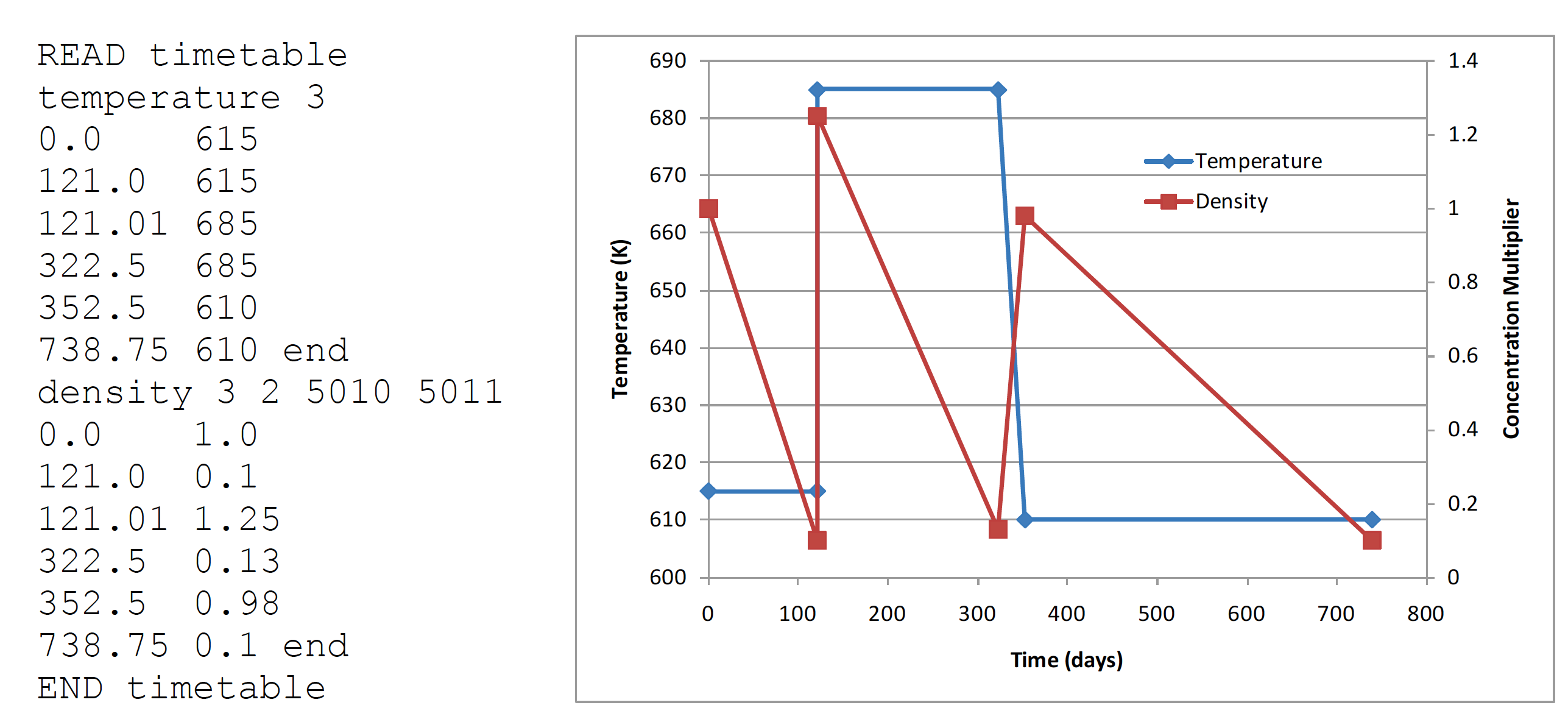
Fig. 3.1.10 Example temperature and density TIMETABLE block input.

Note

It is important to note that time-dependent changes to temperatures and number densities are not applied continuously over the depletion calculation, but instead are applied only at the times at which cross section processing and transport calculations are performed - that is, the midpoint of the depletion subintervals. The user must determine the accurate depletion scheme specific to his or her application to accurately model time-dependent changes in system properties.

Density timetable specifications can be used to effectively exchange compositions of a single material. One may construct a compound material comprised of two distinct materials at their design densities; a timetable specification can be used to set the density multiplier to 1.0 for the nuclides initially present and to use a multiplier of 0.0 for all nuclides in materials that are not intended to be present at time zero. The timetable can then affect the exchange by changing the multipliers from 0 to 1, and from 1 to 0, at the time of the material exchange. One must bear in mind that timetable processing within TRITON performs linear interpolation between time points; if the exchange is intended to occur at a specific moment in time, then the timetable should be set up with the exchange occurring within a very short period. Moreover, it is important to note that material exchanges for two materials that have common nuclides are more difficult to model. For example, a B₄C absorber material and borated H₂O moderator material both contain boron nuclides in common. In order to exchange the B₄C absorber material and the borated H₂O moderator material, the carbon, oxygen, and hydrogen density multipliers would be 0 or 1, but the boron density multipliers would need to be derived from the boron concentrations in both materials.

3.1.3.3.5.2. Material swap

Material exchange timetables offer another option to users to exchange one material with another material during depletion calculations.

Material exchange timetable has a similar format to temperature timetables:

swap I1 I2 t1 S1 t2 S2 t3 S3...tC SC end

where

I1 = first material ID

I2 = second material ID

t_j = time (days) in calculation where swap ID is set, i = 1 to C;

S_j = swap value 0/1 at time t_j, i = 1 to C;

C = number of time steps.

The first two entries in the timetable specify the material IDs for swap materials. The remaining entries are entered in pairs: the first pair value is a time value, the second pair value is either “0” or “1”. “0” instructs TRITON to model the swap materials as defined in the nominal model. “1” instructs TRITON to swap the materials (swap every I1 for every I2 and swap every I2 for every I1). The swap state persists until the next time entry in the timetable. For the last time entry in the timetable, the swap state persists for the duration of the calculation. For example:

read timetable
  swap 5 6  0 0  100 1  200 0 end
read timetable

Do not perform the material swap on the interval [0, 100],
Perform the material swap on the interval [100, 200], and
Return to the nominal state at time 200 days until the duration of the calculation.

Depending on the BURNDATA specification, there may be one or more depletion/decay steps between timetable entries. Moreover, for accurate depletion modeling, material exchanges must not occur during a depletion subinterval. If a material exchange occurs during a depletion interval, TRITON will subdivide the depletion subinterval at the time of the material exchange. Extending the example above, assume the BURNDATA block is as follows:

read timetable
  swap 5 6  0 0  100 1  200 0 end
read timetable
read burndata
 power=40 burn=300 nlib=4 end
end burndata

Without the material exchange table, the depletion subintervals are [0, 75], [75, 150], [150, 225], and [225, 300]. With the material exchange table, the subintervals are:

[0, 75] – Swap value is 0
[75, 100] – Swap value is 0
[100–150] – Swap value is 1, i.e. materials 5 and 6 swap definitions
[150–200] – Swap value is 1, i.e. materials 5 and 6 swap definitions
[200–225] – Swap value is 0, materials 5 and 6 return to their original definitions
[225–300] – Swap value is 0

As a limitation of the material exchange timetable, if a depletion material is removed from the geometry, the isotope concentrations at the time of removal are stored in-memory, and then reused upon re-entry into the geometry. In other words, the depletion material does not undergo radioactive decay for the period of time outside the problem geometry.

3.1.3.3.5.3. Material flow

To allow modeling of systems with flowing fuel, TRITON offers a FLOW block which permits fractional removal and continuous feed from/to mixture. When this block is requested, TRITON makes use of ORIGEN’s capability for feed and removal from/to mixtures, including the decay of nuclides removed from the system. Detailed information about the feed and removal to simulate flowing fuel can be found in [TRITONVBWF20], [TRITONBPW17], [TRITONBPBR17].

Eq. (5.1.1) from the ORIGEN part of the manual (Sect. 5.1.3) is as follows when explicitly adding a removal rate $\lambda_{i,rem}$ and acknowledging the feed rate $S_{i}$:

(3.1.1)\[\frac{dN_{i}}{\text{dt}} = \sum_{j \neq i}{(l_{\text{ij}} \lambda_{j} + f_{\text{ij}}\sigma_{j}\Phi})N_{j}\left( t \right) - \left( \lambda_{i} + \lambda_{i,rem} + \sigma_{i}\Phi \right) N_{i}(t) + S_{i}(t)\]

where

$N_{i}$ = amount of nuclide i (atoms),

$\lambda_{i}$ = decay constant of nuclide i (1/s),

$\lambda_{i,rem}$ = removal constant defining the continuous removal of nuclide i (1/s),

$l_{\text{ij}}$ = fractional yield of nuclide i from decay of nuclide j,

$\sigma_{i}$ = spectrum-averaged removal cross section for nuclide i (barn),

$f_{\text{ij}}$ = fractional yield of nuclide i from neutron-induced removal of nuclide j,

$\Phi$ = angle- and energy-integrated time-dependent neutron flux (neutrons/cm²-s), and

$S_{i}$ = time-dependent source/feed term (atoms/s).

The FLOW block can consider two scenarios: (1) continuous feed into a mixture and (2) fractional removal from one mixture into another.

In the case of the continuous feed, the feed rate (source) must be specified by the user. The feed rate provided in the input is considered as feed into the mixture of mass and volume corresponding to the model’s geometry and as seen by the neutron transport code. When initializing the depletable mixtures in ORIGEN, TRITON normalizes their masses and adjusts the volume accordingly to yield a total mass of 1 metric ton initial heavy metal. Therefore, the user-supplied feed rate is multiplied by the same multiplier before it is provided to ORIGEN.

In the case of the fractional removal of a nuclide from material 1 to material 2, the removal rate (removal constant) for material 1 is specified. The removed nuclides from material 1 are then considered as source for material 2.

The following FLOW block enables continuous feed of nuclides into a mixture:

read timetable
  flow
    to I2
    type continuous_feed
    units [gpers or kgpers or molpers]
    nuclides [N1 N2 ... NM] end
    rates    [R1 R2 ... RM] end
    time       [t1 t2 ... tC] end
    multiplier [f1 f2 ... fC] end
  end flow
end timetable

The following FLOW block enables fractional removal of nuclides from one mixture to another:

read timetable
  flow
    from I1
    to I2
    type fractional_removal
    units pers
    nuclides [N1 N2 ... NM] end
    rates    [R1 R2 ... RM] end
    time       [t1 t2 ... tC] end
    multiplier [f1 f2 ... fC] end
  end flow
end timetable

The input parameters are as follows:

I = mixture ID
from = identifier from which mixture nuclides are removed (from I1)
- required for flow blocks with fractional_removal
- not permitted for flow blocks with continuous_feed
to = identifier to which mixture nuclides are added (to I2)
type = type of addition or removal of nuclides from/to mixture:
- fractional_removal requires from and to
- continuous_feed requires to and does not permit from
units = unit of the flow rate constant used:
- for flow blocks with fractional_removal: pers (1/second)
- for flow blocks with continuous_feed: gpers (grams/second), kgpers (kilograms/second), molpers (moles/second)
M = number of nuclides to which change is applied
N_i = nuclide ID for the i_th nuclide in the list, i = 1 to M
- specification of elements, specific nuclides, and keyword all is permitted
R_i = rates for the i_th nuclide in the list, i = 1 to M
C = number of time steps
t_j = time (days) in calculation where multiplier f_j is set, i = 1 to C, t1 must be 0.0
f_j = multiplier to vary specified flow rate (based off the initial flow rate) at time t_j, i = 1 to C

Note

Just as for temperature and density changes, TRITON applies linear interpolation between the data provided at specific times. To hold a rate/multiplier pair constant over a time interval, that rate/multiplier pair should be specified at the same value at both the beginning and the end of this time interval.

Special cases in the nuclide array

In case of overlapping specifications in the nuclide block, the assigned rates are processed in the order all->element->nuclide. For example, the input

nuclides    u   all u-235  end
rates    1e-3  1e-4  1e-5  end

is processed in the following order:

assign rate 1e-4 to all

assign rate 1e-3 to u

assign rate 1e-5 to u-235

In this way, a rate of 1e-5 is assigned to U-235, a rate of 1e-3 is assigned to all uranium isotopes besides U-235, and a rate of 1e-4 is assigned to all nuclides besides all uranium isotopes. The order in which all, elements, and nuclides are specified is irrelevant.

Nuclide removal and feed interaction

If nuclides are transferred from mixture 1 into mixture 2—that is, they are removed from mixture 1 and fed into mixture 2—then users might observe slight inconsistencies in the removed compared to the fed nuclide amounts after a TRITON depletion/decay step. The removal of nuclides is handled exactly according to the expected behavior with the assigned removal rate. This means that in the absense of any other nuclide production or removal mechanism, the nuclide density in mixture 1 would follow:

(3.1.2)\[\frac{dN_{i}}{\text{d}t} = - \lambda_{i,rem} N_{i}(t)\]

In order to connect the removal from material 1 to the feed rate into material 2, the removal is integrated numerically over a substep and recast as a nuclide feed for this specific substep s:

(3.1.3)\[S_{i,s} = \int_{t_{s-1}}^{t_s} \lambda_{i,rem}N_{i}(t) \text{d}t\]

The approximation for N_i over a substep uses a weighted essentially non-oscillatory (WENO)–like scheme that takes the nuclide amounts at the beginning and end of a substep and determines a combination of logarithmic and linear interpolation, preferring logarithmic if the amounts differ greatly and linear if they are similar. If there are particularly strong removals, then it may be necessary to introduce additional small time steps (i.e., additional depletion/decay steps in the BURNDATA block) to better handle the numerical integration on the substeps.

Decay of mixtures outside of the system

If nuclides are transferred from mixture 1 into mixture 2, but mixture 2 is not part of the system (e.g., contained in a loop outside the reactor), then the decay of the nuclides in this mixture can still be considered by specifying keyword decayonly in the DEPLETION block.

These decayonly mixtures exist only on the ORIGEN side, but they are not relevant for the neutron transport calculation. Their volume is by default set to 1 cm³, and their mass is set according to the specified density for this volume. TRITON’s mass normalization does not affect the volumes or masses of these mixtures. However, if a continuous_feed is applied to such a mixture, then the specified feed rate is still multiplied with the multiplier used for the mass normalization.

The following is an example in which xenon is transfered from mixture 1 to mixture 2, and the decay of nuclides in mixture 2 is enabled in the DEPLETION block:

read depletion
-1 decayonly 2
end depletion

read timetable
  flow
   from 1
   to 2
   type fractional_removal
   units pers
   nuclides    xe end
   rates     2e-2 end
   time       0.0 end
   multiplier 1.0 end
 end flow
end timetable

3.1.3.3.6. OPUS block

The OPUS module of SCALE is fully documented in the OPUS chapter of the SCALE manual. OPUS provides the ability to extract specific data from ORIGEN output libraries, perform unit conversions, and generate plot data for post-calculation analysis. In essence, OPUS is an ORIGEN post-processor that provides data in the desired form for a desired subset of nuclides. TRITON by default calls OPUS to extract nuclide concentrations for selected nuclides for all depletion materials and for the most important nuclides. TRITON provides the capability to specify the full set of OPUS commands to tailor OPUS calculations to obtain specific information. TRITON allows a stacked set of OPUS calculations in order to retrieve selected data for selected nuclides.

The content of the OPUS block is based on standard OPUS input parameters, as described in the OPUS chapter; the details of OPUS control and use are not repeated here. However, additional input is necessary to support TRITON operations with OPUS, because TRITON enables additional capabilities beyond those provided for in standard OPUS input. For example, OPUS is designed to process the output file from a single ORIGEN calculation; because ORIGEN is a point depletion solver, the output represents data from a single material. TRITON is typically used to perform multiple depletion calculations at each depletion step-one calculation for each material being depleted. Hence, multiple OPUS calculations are needed to obtain results from multiple materials. The OPUS calculations are performed automatically by TRITON but require the user to specify the materials for which OPUS processing is desired. Additionally, TRITON supports stacked OPUS cases within the READ OPUS data block; hence, keywords are introduced to separate stacked cases.

There are two alternatives available to SCALE users that are complimentary to the OPUS block within TRITON. First, standalone OPUS case(s) can be used to post process the ORIGEN binary concentration file (.f71 extension). This file is automatically saved in the output directory with the file name ${OUTBASENAME}.f71. (e.g. if the input file is reactor.inp, the concentration file is saved in the output directory as reactor.f71) Second, the user may also open the concentration file within Fulcrum to enable similar post-processing capabilities.

3.1.3.3.6.1. Selection of materials for OPUS processing

Beyond standard OPUS input keywords (see OPUS chapter), TRITON reads a matl= keyword to allow specification of ID number(s) for the material(s) in the problem for which outputs are desired. The matl=…end input keyword accepts one or more materials from the DEPLETION data block for which OPUS processing is desired. If omitted, OPUS processing will be performed for all materials in the DEPLETION block. For example, consider the following DEPLETION and OPUS data blocks:

READ depletion 1 2 3 4 5 6 END depletion
READ opus
units=gram symnuc=u-234 u-235 u-236 u-238 pu-238 pu-239
pu-240 pu-241 pu-242 pu-243 np-237 end
time=year
END opus

In this example, OPUS processing will be performed for all depletion materials, 1–6. Adding a subset of materials using the matl= keyword, for example.

READ depletion 1 2 3 4 5 6 END depletion
READ opus
units=gram symnuc=u-234 u-235 u-236 u-238 pu-238 pu-239
pu-240 pu-241 pu-242 pu-243 np-237 end
time=year
matl=1 2 3 end
END opus

will result in OPUS calculations for materials 1, 2, and 3 only.

Although ORIGEN calculations are performed only for individual materials, TRITON provides the capability of combining the results of all or a subset of all depletion materials to get a multimaterial average set of ORIGEN responses. TRITON provides three special ID numbers for combining material results:

material ID 0 returns system-averaged results for the entire set of depletion materials (i.e., all mixtures included in the depletion block),

material ID -1 returns the average of only those materials with ID > 0 present in OPUS matl= list,

material ID -2 returns averaged results for all fuel materials in the system (i.e., all mixtures with a non-negligible heavy metal mass)

Again, this is best illustrated by example. Specification of the data blocks

READ depletion 1 2 3 4 5 6 END depletion
READ opus
units=gram symnuc=u-234 u-235 u-236 u-238 pu-238 pu-239
pu-240 pu-241 pu-242 pu-243 np-237 end
time=year
matl=1 2 3 0 -1 end
END opus

will result in five OPUS calculations and five sets of results-one for each of materials 1, 2, and 3, one for the average of materials 1–6 (due to input of material ID 0), and one for the average of materials 1–3 (due to input of material ID –1).

3.1.3.3.6.2. Specification of stacked OPUS cases

In a given calculation, multiple output units may be desired (e.g., grams, curies, and watts), or multiple time scales (e.g., seconds and years), or a combination of these or other parameters. TRITON provides the ability to stack inputs such that multiple cases may be run within a single TRITON calculation. In order to stack cases, the keywords new case are entered in the input stream. Any parameters following these keywords are used to define a new OPUS case.

There is no limit on the number of stacked cases that may be input; however, the matl= specification may be used only in the first case. OPUS calculations are run for each of the materials in this list, for all cases.

Consider a depletion calculation where gadolinium pins are present in the assembly design. One may wish to determine the quantities of gadolinium nuclides from the initial poison rods (tracked as a light element by ORIGEN within TRITON) and from fission (tracked as a fission product by ORIGEN). One may also need masses of selected actinides as well as the total ($\alpha$,n) reaction rate. Fig. 3.1.11 shows how the new case keyword set is used to define unique OPUS calculations. In this example, the new case keywords are shown in upper case and on a line by themselves, but this has been done only for readability. The text may be entered in lower case and on the same line as other keywords. Note, however, that the matl= specification is given only in the first case. All OPUS calculations will be performed for materials 1, 2, and 3 and for the average of these three materials.

Fig. 3.1.11 Example OPUS block input.

3.1.3.3.7. TALLIES and DEFINITIONS block

As of SCALE 6.3, a TALLIES input block and a DEFINITIONS input block can be used with CSAS-Shift and TRITON-Shift for flexible definition and output control of mesh tallies. The mesh responses for neutron flux, the neutrons produced from fission, and the fission rate (new since 6.3) can be requested on different spatial and energy grids. The syntax is very similar to the corresponding blocks used in the MAVRIC sequence.

The input parameters previously used to request these responses (i.e., gfx, cds, and fis) are still permitted in SCALE 6.3, but it is recommended to use the new input. The new input further permits the mesh tally responses based on different spatial grids and energy grids within one calculation, whereas previously only one spatial and energy grid was permitted per calculation.

DEFINITIONS BLOCK

The new definitions input block allows multiple spatial grids to be defined using the gridGeometry keyword and multiple energy grids to be defined using the energyBounds keyword. The syntax for defining a gridGeometry inside a definitions block is the same as defining a standalone grid at the root level of input (see Sect. 8.1.3.14). Additionally, TRITON supports infinite meshes (“nets”) over the whole geometry for the generation of nodal data with the fgxs block. For the purpose of nodal data generation, individual shapes are now permitted as well.

Spatial definitions are defined as follows:

read definitions

  read grid 1
      type=planar
      xlinear 30 -10 70
      ylinear 10 -20 60
      zlinear 50 -30 40
  end grid

  read grid 2
      type=planar
      numxcells=10 xmin=-18.5 xmax=+68.5
      numycells=25 ymin=-28.5 ymax=+58.5
      numzcells=10 zmin=-38.5 zmax=+48.5
  end grid

  read grid 3
      type=square_net
      boundary=global_unit
      pitch=2.5
      origin x=0 y=0.5
      zplanes 100.0 50.0 0.0 -20.0 end
  end grid

  read grid 4
      type=hex_net
      rotate=yes
      boundary=global_unit
      hpitch=0.5
      origin x=0 y=0.5
      zlinear 10 100.0 -20.0
  end grid

  read shape 1
      cuboid 5.0 -5.0 5.0 -5.0 1.0 0.0
  end shape

  read shape 2
      rhexprism 1.25 2.0 -2.0 origin x=0 y=0
  end shape

end definitions

The square and hexagonal infinite meshes requested through square_net and hex_net, respectively, are used only in combination with the fgxs block for the generation of nodal data. Since only rotated hexagonal meshes are permitted at this point, parameter rotate is currently required to be set to yes. These nets must be further specified to cover the whole geometry. Therefore, the boundary is at this point required to be global_unit.

Note

For TRITON-Shift sequences, the grid boundaries must be inside the specified geometry, while TRITON-KENO permits the grid boundaries to go beyond the geometry.

Individual cuboids and rotated hexagonal prisms can be requested through the shape sub-block. These are used only in combination with the fgxs block for the generation of nodal data. The syntax for these shapes follows the syntax for the corresponding standard KENO/Shift geometry input.

Energy grids are defined as follows:

read definitions

' global energy grid, default is 252g in CE mode, but can be modified here
  energyBounds default
      bounds 2e7 0.625 1e-5 end
  end energyBounds

' user specified energy grid
  energyBounds 1
      bounds 2e7 0.625 1e-5 end
  end energyBounds

' user specified energy grid using equal-energy bins
  energyBounds 2
      linear=10 1e-5 2e7
  end energyBounds

' user specified energy grid using equal-lethargy bins
  energyBounds 3
      logarithmic=10 1e-5 2e7
  end energyBounds

  'SCALE 56-group neutron structure with additional energy points
  energyBounds 10
     56n
     bounds 1.1  0.11 0.011 0.0011 end
  energyBounds

end definitions

The syntax for defining energyBounds is already used for defining energy grids in the MAVRIC sequence (see Table 8.2.12). The energy grid definition permits specification of individual energy boundaries, equal-width energy bins and equal-width lethargy bins within a specified energy, and SCALE energy group structures (such as the 56-group structure). The SCALE energy group structure can be any group structures that is used by a SCALE multigroup library that is available in the DATA directory. The syntax is <num>n for neutron libraries and <num>p for photon (gamma) libraries. A combination of the different options is also supported.

In continuous-energy mode, a special default keyword allows modification of the default energy group structure previously defined with the NGP parameter and/or the standalone energy block. For example, TRITON-Shift can use these energyBounds to tally flux and cross sections for depletion calculations.

TALLIES BLOCK

The new tallies input block allows specific responses to be requested using energy grid and/or spatial grid from the definitions block. There are currently two types of tallies: mesh tallies and fgxs tallies. The mesh tallies allow the tallying of the neutron flux, the fission rate, or the neutrons produced from fission. The results are provided in 3dmap files. The fgxs tallies allow the generation of nodal data for use in nodal diffusion codes when TRITON is used in combination with Shift in CE mode. The results are provided in T16 text files and HDF5 files.

Note that mesh tallies were previously supported through parameters in the parameters block, as listed in Table Table 3.1.3.

TRITON-Shift allows specifying a time input array to enable or disable these tallies for specific depletion steps. The last depletion step may be conveniently requested using the special LAST keyword, and the special ALL keyword may be used to request the tally for every depletion step.

Table 3.1.3 Mesh tallies available within the **tallies** block.
Description	SCALE 6.2 parameter name	SCALE 6.3 parameter name
neutron flux	GFX	flux
fission rate	FIS	fission_density
neutrons produced from fission	CDS	fission_source

The following examples demonstrate how the TALLIES block is used in TRITON-KENO and TRITON-Shift calculations with a mesh response:

read tallies

  read mesh 1
      response = FLUX
      grid     = 1
      time       0 LAST end
      energy   = 1
  end mesh

  read mesh 2
      response = FISSION_DENSITY
      grid     = 2
      time       0 1 2 end
      energy   = 2
  end mesh

  read mesh 3
      response = FISSION_SOURCE
      grid     = 3
      time       ALL end
      energy   = default
  end mesh

end tallies

The following examples demonstrate how the TALLIES block is used in TRITON-Shift CE calculations with a fgxs response:

read tallies

    read fgxs 1
        response=macro_nodal
        grid=2
        time 0 1 2 LAST end
        energy=5
    end fgxs

    read fgxs 2
        response=macro_nodal
        shape=1
        time ALL end
        energy=5
    end fgxs

end tallies

The only response that is currently supported for this tally type is macro_nodal.

On overview of the individual tallies that are set up in Shift through a fgxs block can be found in the output file. For example:

=============================================================================================
Nodal FGXS Tally Summary
=============================================================================================

  Tally ID=30
    tally spatial type: MESH
    tally boundary: RHEXPRISM
    energy grid: 2e+07,0.625,1e-05
    volume mesh inscribed radius: 0.500000
    volume mesh center: -0.288675,-0.5
    volume mesh planes z: -1e-06,0.9,1
    volume tallies: absorption,fission,flux,kappa_sigma,nu_delayed_fission,nu_fission,transfer_1n,transfer_2n,transfer_3n,transfer_4n
    volume tallies on isotopes (nuclide id/reaction mt): 1001/18, ... , 96245/1018
    fine energy grid: 2e+07,... , 1e-05
    fine energy grid volume tallies: flux,absorption,fission,transfer_1n,transfer_2n,transfer_3n,transfer_4n
    volume tally name (shift): mesh_nodal_tally_t16_30
    num tally energy groups: 2
    num tally mesh rings: 2
    num tally fine energy groups: 1000

  Tally ID=40
   ...

The t16 output file names are composed of the ${BASENAME} of the input file, the tally id, the mesh ids in case of global meshes, and they have the ending t16.

The output t16 and HDF5 output files are named according to the fgxs tally id. For nodal data requested over a mesh, an individual file is created per mesh voxel. The following syntax applies:

fgxs tally over a shape: ${BASENAME}.id<id>.t16, ${BASENAME}.id<id>.nodal.h5

fgxs tally over a square mesh: ${BASENAME}.id<id>-<x>-<y>-<z>.t16, ${BASENAME}.id<id>-<x>-<y>-<z>.nodal.h5

fgxs tally over a hexagonal mesh: ${BASENAME}.id<id>-<ii>-<jj>-<kk>.t16, ${BASENAME}.id<id>-<ii>-<jj>-<kk>.nodal.h5

Although the x/y/z locations of the square mesh are self-explanatory and the origin of the individual mesh voxels can be derived through the “FGXS Tally Summary”, a visual representation of the mesh superimposed on the geometry is printed for hexagonal meshes. This print-out also contains an overview of all file names with the corresponding (x,y)-origin of the cells and the axial range, for example:

T16 file summary for hex mesh tally id=4
=========================================

Apothem (inner radius):        0.5 cm
Number of rings: 2
Grid size: 5

basename.id4-<II>-<JJ>-<KK>.t16              x              y           zmin           zmax
---------------------------------------------------------------------------------------------------------
      basename.id30-02-04-01.t16   -1.15470e+00    0.00000e+00   -1.00000e-06    9.00000e-01
      basename.id30-02-04-02.t16   -1.15470e+00    0.00000e+00    9.00000e-01    1.00000e+00
      basename.id30-03-03-01.t16   -2.88675e-01   -5.00000e-01   -1.00000e-06    9.00000e-01
      basename.id30-03-03-02.t16   -2.88675e-01   -5.00000e-01    9.00000e-01    1.00000e+00
      basename.id30-03-04-01.t16   -2.88675e-01    5.00000e-01   -1.00000e-06    9.00000e-01
      basename.id30-03-04-02.t16   -2.88675e-01    5.00000e-01    9.00000e-01    1.00000e+00
      basename.id30-04-02-01.t16    5.77350e-01   -1.00000e+00   -1.00000e-06    9.00000e-01
      basename.id30-04-02-02.t16    5.77350e-01   -1.00000e+00    9.00000e-01    1.00000e+00
      basename.id30-04-03-01.t16    5.77350e-01    0.00000e+00   -1.00000e-06    9.00000e-01
      basename.id30-04-03-02.t16    5.77350e-01    0.00000e+00    9.00000e-01    1.00000e+00
      basename.id30-04-04-01.t16    5.77350e-01    1.00000e+00   -1.00000e-06    9.00000e-01
      basename.id30-04-04-02.t16    5.77350e-01    1.00000e+00    9.00000e-01    1.00000e+00

                              _____
                             /     \
                       _____/ 05    \
                      /     \ 05    /
                _____/ 04    \_____/
               /     \ 05    /     \
         _____/ 03    \_____/ 05    \
        /     \ 05    /     \ 04    /
  _____/ 02    \_____/*04****\_____/
 /     \ 05    /     \*04****/     \
/ 01    \_____/*03****\_____/ 05    \
\ 05    /     \*04****/     \ 03    /
 \_____/*02****\_____/*04****\_____/
 /     \*04****/     \*03****/     \
/ 01    \_____/#03####\_____/ 05    \
\ 04    /     \#03####/     \ 02    /
 \_____/ 02    \_____/*04****\_____/
 /     \ 03    /     \*02****/     \
/ 01    \_____/ 03    \_____/ 05    \
\ 03    /     \ 02    /     \ 01    /
 \_____/ 02    \_____/ 04    \_____/
 /     \ 02    /     \ 01    /
/ 01    \_____/ 03    \_____/
\ 02    /     \ 01    /
 \_____/ 02    \_____/
 /     \ 01    /
/ 01    \_____/
\ 01    /
 \_____/

#### mesh origin cell
**** tally cells
<II> cell column/x-index
<JJ> cell row/y-index

3.1.3.4. ALIAS block

The optional ALIAS block may be used to simplify model development within TRITON by defining a set of material numbers that will be inserted in place of the alias when that alias is used in subsequent data blocks. Aliases function as variables for which a user-defined set of materials are inserted; they are identified by a dollar character ($) preceding a single-word alphanumeric label. The ALIAS block is used to preprocess an input, creating a new, modified input deck with all alias variable substitutions included. TRITON then processes the modified input deck before proceeding with the calculation.

The use of an alias variable is best illustrated by a brief example. Assume that the alias $fuel is defined as materials 1, 2, and 3, and $mod as materials 4, 5, and 6. (The input format for defining aliases is described below.) The user wishes to create three identical sets of materials and use them in three identical pin cell specifications. In the COMPOSITION data block, specifications could be written in the following form

h2o $mod den=0.6616 1.0 595 end
wtpt-boron $mod 0.6616 1 5000 100 655e-6 595 end

TRITON would create a modified input with the alias expanded as follows:

uo2  1 den=10.29 0.9322 920 92235 3.0 92238 97.0 end
uo2  2 den=10.29 0.9322 920 92235 3.0 92238 97.0 end
uo2  3 den=10.29 0.9322 920 92235 3.0 92238 97.0 end
h2o 4 den=0.6616 1.0 595 end
h2o 5 den=0.6616 1.0 595 end
h2o 6 den=0.6616 1.0 595 end
wtpt-boron  4 0.6616 1 5000 100 655e-6 595 end
wtpt-boron  5 0.6616 1 5000 100 655e-6 595 end
wtpt-boron  6 0.6616 1 5000 100 655e-6 595 end

Similarly, if the alias were used in the CELLDATA block as

latticecell squarepitch pitch=1.26 $mod fuelr=0.4095 $fuel end

then TRITON would expand the aliases to

latticecell squarepitch pitch=1.26 4 fuelr=0.4095 1 end
latticecell squarepitch pitch=1.26 5 fuelr=0.4095 2 end
latticecell squarepitch pitch=1.26 6 fuelr=0.4095 3 end

In a depletion calculation, one may wish to deplete a large number of fuel rods independently because of different geometric locations in a fuel assembly. Even though each fuel rod may have the same initial composition, each must be specified as a unique material composition in order to be depleted independently. Furthermore, multiple cell specifications must all use unique material identifiers for each cell component. Thus, if one desired to deplete 25 fuel materials in a fuel/clad/moderator pin cell, one would need to set up material composition definitions for 25 fuels, 25 moderators, and 25 clads. Then one would need to provide 25 pin cell specifications. By using aliases, one need only specify the material identifiers corresponding to each alias and then provide only one material composition specification for each alias type, and then one pin cell specification. TRITON will automatically expand the aliases and create a revised input with all materials and cell specifications explicitly defined.

Note

Note that although this will simplify the pin cell input in the CELLDATA, 25 pin cell calculations would still be required. The number of pin cell calculations can be reduced by using the ASSIGN function described in Sect. 3.1.3.3.4.3.

The purpose of the ALIAS block is to define a set of alias variables to be used in subsequent data blocks. The ALIAS block is optional, but aliases may not be used in other blocks if an ALIAS block is not present to define the aliases. An ALIAS block may contain as many aliases as desired. Each alias specification consists of three parts: the alias name, consisting of a dollar sign followed by up to 11 alphanumeric characters with no embedded spaces; the material number or numbers; and an end keyword. Material numbers may be entered in any order and may be separated by spaces or commas (or both). Material numbers may also be separated by a dash (-), but this represents an inclusive list. In other words, a material specification of 1-3 (or 1 - 1) indicates materials 1, 2, and 3. The example ALIAS block below illustrates the various means for assigning a set of materials for an alias definition.

read alias
$fueltype1 1 2 3 end
$fueltype2 4,5,6, 31-33 end
$clad1 21,22,23 end
$clad2 24 25 26 34-36 end
$mod1 11    -   13 end
$mod2 14-16, 37-39 end
end alias

The ALIAS block simply serves to assign material identifiers to specific variables, and the variables are used in subsequent data blocks. The same material identifier can be used in more than one alias if desired. As indicated earlier, TRITON will preprocess any input deck containing an ALIAS block and replace instances of alias variables with the appropriate material identifiers. The following subsections describe how aliases are implemented in TRITON’s various input blocks, as the form of alias variable substitution is block dependent. Aliases are processed only in these input blocks; aliases used in other blocks will result in an error.

3.1.3.4.1. COMPOSITION block aliases

The COMPOSITION block uses aliases to create multiple copies of each standard composition specification, replacing the alias variable with each material identifier associated with the alias definition. For example, consider the following alias definition in an ALIAS block:

read alias
$fuel 1 2 10 end
end alias

and the standard composition specification:

uo2 $fuel den=10.045 1 800 92235 2.5 92238 97.5 end

A modified TRITON input would be created with the standard composition specification replaced by

uo2  1 den=10.045 1 800 92235 2.5 92238 97.5 end
uo2  2 den=10.045 1 800 92235 2.5 92238 97.5 end
uo2 10 den=10.045 1 800 92235 2.5 92238 97.5 end

3.1.3.4.2. CELLDATA block aliases

CELLDATA block latticecell specifications typically contain more than one material; therefore, multiple aliases are permitted in each cell specification. However, this constrains the set of aliases used in the cell specification to have the same number of material identifiers associated with it.

Consider the ALIAS block:

read alias
$fuel 1-3 10 end
$clad 4,5,6,11 end
$mod 7 8-9 12 end
end alias

All three aliases contain four materials each. One could then create a single cell specification that uses one or more of these alias variables, such as

latticecell squarepitch pitch=1.26 $mod fuelr=0.41 $fuel cladr=0.50 $clad end

This would result in the following alias expansion by TRITON:

latticecell squarepitch pitch=1.26  7 fuelr=0.41  1 cladr=0.50  4 end
latticecell squarepitch pitch=1.26  8 fuelr=0.41  2 cladr=0.50  5 end
latticecell squarepitch pitch=1.26  9 fuelr=0.41  3 cladr=0.50  6 end
latticecell squarepitch pitch=1.26 12 fuelr=0.41 10 cladr=0.50 11 end

Material identifiers are substituted according to their position in the alias definition (i.e., the first substitution will use the first material associated with each alias, and the second expansion will use the second material associated with each alias, etc.)

Material numbers should not be entered manually in a cell specification; for example,

latticecell triangpitch pitch=1.26 $mod fuelr=0.4095 1 end

TRITON would allow this to occur and would create a set of cell specifications as follows:

latticecell triangpitch pitch=1.26 2 fuelr=0.4095 1 end
latticecell triangpitch pitch=1.26 3 fuelr=0.4095 1 end

where $mod was defined as materials 2 and 3. However, SCALE does not allow the same material identifier to occur in two different cell specifications, and the fact that material 1 occurs in two different cell specifications would result in TRITON ending with an error. Note that alias expansions formultiregionanddoublehetcell specifications are not supported. Also note that TRITON will not copycentrmdataandmoredataspecifications that follow a cell specification that uses an alias variable.

3.1.3.4.3. DEPLETION block aliases

Aliases in the TRITON DEPLETION are simply replaced by the set of materials associated with the alias. For example, the ALIAS block

read alias
$fuel 1 2 10 end
end alias

and DEPLETION block

read depletion 7 8 9 $fuel end depletion

would be expanded to

read depletion 7 8 9 1 2 10 end depletion

Aliases may be mixed with actual material numbers in the depletion block, along with the flux and assign keywords. However, the negative sign-used to define the basis for power normalization-cannot precede an alias definition.

3.1.3.4.4. TIMETABLE block aliases

TIMETABLE block alias expansion is similar to that of the COMPOSITION block: TRITON will create a new timetable entry for each material associated with the alias used in the TIMETABLE definition. For the TIMETABLE block below, using the alias $allmod, unique timetables will be created for each material identifier associated with this alias variable.

Note

Note that alias expansion of density timetable entries is not yet supported.

read timetable
temperature $allmod
0.0    615
121.0  615
121.01 685
322.5  685
352.5  610
738.75 610 end
end timetable

3.1.3.4.5. BRANCH block aliases

Aliases may be used within the define keyword definitions of the BRANCH block. Aliases are simply replaced by the list of materials associated with the alias, as is done for the DEPLETION block. Hence,

read alias
$fuel 1 2 10 end
end alias

used with

read branch
define fuel $fuel end
md=0.75 tm=559 tf=880 sb=0.0 cr=0 end
tf=1600 end
end branch

would be expanded to

read branch
define fuel 1 2 10 end
md=0.75 tm=559 tf=880 sb=0.0 cr=0 end
tf=1600 end
end branch

3.1.3.4.6. NEWT MATERIAL block aliases

The MATERIAL block within the NEWT model section of a TRITON input can also use aliases. As with COMPOSITION and TIMETABLE entries, TRITON will create a new material specification for each material represented by an alias. For the sample material block below, using the alias $fuel, unique material block entries will be created for each material associated with the alias variable.

read materials
mix=$fuel pn=1  com="3.25 wo uo2 fuel" end
mix=21    pn=1  com="zirc cladding"    end
mix=31    pn=1  com="water"            end
end materials

If an alias were defined as

$fuel 10 11 12 end

then the MATERIAL block would be expanded to

read materials
mix=10 pn=1  com="3.25 wo uo2 fuel" end
mix=11 pn=1  com="3.25 wo uo2 fuel" end
mix=12 pn=1  com="3.25 wo uo2 fuel" end
mix=21    pn=1  com="zirc cladding"    end
mix=31    pn=1  com="water"            end
end materials

3.1.3.4.7. KEEP_OUTPUT block

When performing depletion calculations for a number of different materials, TRITON output can become quite voluminous. Often, much of that output is not needed for calculations that seek only eigenvalues, sources, or concentrations as a function of irradiation history. TRITON provides the ability to trim output to only those portions for which output is desired. Output produced directly by the TRITON module is always provided and cannot be disabled, but output from any other code in the sequence can be removed from the output listing. Retaining certain output is accomplished using the KEEP_OUTPUT data block.

The KEEP_OUTPUT data block provides the ability to preserve only selected outputs. The format of this data block is

read keep_output
  module_1 [time array] end
  ...
  module_i [time array] end
  ...
  module_N [time array] end
end keep_output

where module_i represents any valid module name from the list of modules invoked by TRITON, as listed here:

xsproc xsdrn newt kenova kenovi shift couple origen kmart

Without the KEEP_OUTPUT data block, the output from the neutron transport kernel (xsdrn, newt, kenova, kenovi) is retained and the output of all other modules (xsproc, couple, origen) is suppressed. Note that the output of SAMS and OPUS is not controlled by this block; the output of these modules is always retained.

If a KEEP_OUTPUT data block is included in the input file, then the user must specify time steps for each module listed in the block. The time array permits the following values:

integer or array of integers to keep the output at the listed individual time steps

special keyword ALL to keep the output at all time steps

special keyword LAST to keep the output at the last time step

special keyword NONE to disable the output completely

The default for a module remains the same if the module name is not listed in the block code. For the transport modules, this means that their output will be retained if the transport module name is not listed in the KEEP_OUTPUT block. For the non-transport modules, this means that their output will not be displayed if the module name is not listed in the KEEP_OUTPUT block.

Note that the first time step of a TRITON calculation is time step 0.

When using the TRITON-Shift sequence, specification of the transport module name “shift” controls both the printed output of the neutron transport module and the generation of Shift’s HDF5 output files.

Examples:

Only the output of the neutron transport kernel is retained:

The input does not contain a KEEP_OUTPUT data block.

Only the XSProc output is retained; the output of the neutron transport kernel, KENO-VI, is suppressed:

read keep_output
  xsproc ALL  end
  kenovi NONE end
end keep_output

The output of both XSProc and the neutron transport kernel, KENO-VI, is retained:

read keep_output
  xsproc ALL end
  kenovi ALL end
end keep_output

The output of all modules is suppressed:

read keep_output
  kenovi NONE end
end keep_output

The outputs of the neutron transport kernel, ORIGEN, and COUPLE are retained at specific time steps:

read keep_output
  kenovi  0 2 LAST end
  origen  2 4 LAST end
  couple LAST end
end keep_output

3.1.3.5. TRITON control parameters

TRITON supports the following of control parameter options:

parm=
CHECK, CENTRM, 2REGION, XSLEVEL=N, WEIGHT, WEIGHT=N, ADDNUX=N, INFDCUTOFF=X, CXM=N, MAXDAYS=N

If an invalid control parameter option is specified, including misspelled keywords, an error message will be generated and execution terminated. TRITON also provides the ability to nest several control parameter keywords together; to combine keywords (where appropriate), a list may be entered, enclosed in parentheses, and separated by commas. For example, to specify CHECK, 2REGION, and ADDNUX=1 at the same time, input would begin with

=t-depl  parm=(check, 2region,addnux=1)

The following subsections provide more detail on each of the control parameters listed above.

3.1.3.5.1. Check mode: parm=check

Specification of parm=check will request that TRITON read all input and ensure that no input errors are present, without running additional calculations. In this mode, all input is set up as if a full calculation will be run, but the sequence exits without any functional module execution. The check mode is useful for debugging or obtaining processed standard composition data, without actually running a calculation. It can also be used to generate plot files for embedded NEWT and KENO inputs for additional review and checking of input specifications. Of course, some errors may be uncovered only by dynamically executing the functional modules; hence, there are rare occasions where a parm=check run will complete with no errors but will fail when run outside of check mode as the problem begins to run.

3.1.3.5.2. Multigroup cross section processing options

The most common use of parm= sequence control is in the selection of an alternate multigroup cross section processing mode.

By default, XSProc enables both the BONAMI and CENTRM modules for cross section processing. BONAMI-only XSProc calculations can be performed using the control parameter parm=bonami.

TRITON also supports the control parameter parm=(xslevel=N). The xslevel parameter option initializes various CENTRM options for the XSProc calculations. The xslevel option is equivalent to initializing all unit cell calculations with the following centrmdata specifications:

parm=(xslevel=1):
centrmdata
  npxs=5 nfst=0 nthr=3 nmf6=-1 alump=0.3 demin=0.125 pmc_omit=1 pmc_dilute=5.0e5
end centrmdata
parm=(xslevel=2):
  centrmdata npxs=5 nfst=0 nthr=3 nmf6=-1 end centrmdata
parm=(xslevel=3):
   centrmdata alump=0.3 demin=0.125 pmc_omit=1 pmc_dilute=5.0e5 end centrmdata
parm=(xslevel=4):
   [no centrmdata statement]

The option parm=(xslevel=4) is equivalent to parm=centrm. The option parm=(xslevel=3) is the default for depletion sequences and is equivalent to parm=centrm but with some minor approximations to decrease run time. The option parm=(xslevel=2) is equivalent to parm=2region for all sequences.

Note that the xslevel=1 and xslevel=3 options have additional specifications for keywords alump, demin, pmc_omit, and pmc_dilute. These keywords are further discussed in the XSProc chapter. The additional keyword specifications are used to decrease run-time for the CENTRM and PMC calculations. Internal investigations have shown that the approximations introduced by the additional keyword specifications have minimal impact on solution accuracy for a wide range of calculations. Therefore the additional keyword specifications are used by default for depletion calculations, where several CENTRM and PMC calculations are necessary. The additional keyword values are not used by default for nondepletion calculations to be consistent with the SCALE CSAS5 and CSAS6 criticality sequences.

3.1.3.5.3. Creating a broad group library: parm=weight, parm=(weight=N)

Used in tandem with the TRITON T-NEWT sequence, the specification parm=weight extends the sequence by setting up and executing the MALOCS2 module to generate a weighted broad-group cross-library (AMPX master format). The spectrum generated in the NEWT transport calculation is used as the weighting function for the collapse. Additionally, the broad-group library energy structure is defined by the NEWT COLLASPE block.

The parm=weight option uses the problem-averaged flux spectrum for the weighting function in the collapse. The problem may be a simple pin cell or a full assembly. However, there may be cases where the flux in a specific region or material is most appropriate for the spectral collapse. TRITON allows identification of a specific material from which the collapsing spectrum should be used. When specified in the form parm=(weight=N), the average flux determined for material N is used in place of the total domain spectrum to perform the collapse.

TRITON sample problem 1 (Sect. 3.1.6.1) provides an example of the use of T-NEWT to produce a new broad-group library. Note that the broad-group library produced in this calculation will reside in the SCALE temporary working directory with the name newxnlib at the end of the calculation. If the library will be needed for future calculations, the user should use a shell script to copy the library back to a more permanent location, and perhaps give it a more meaningful name. In sample problem 1, the SCALE 252-group master library is collapsed to 56 energy groups.

The process for creating a broad-group master library is also supported in the 2D depletion sequence T-DEPL. When parm=weight or parm=(weight=N) is specified in a depletion calculation, the input cross section library must be one of the SCALE 238-group or 252-group libraries, which will automatically be collapsed to the SCALE 49-group or 56-group structure, respectively. An initial fine group calculation is performed for the input configuration, and the flux from the solution is used to create the broad group library. The initial calculation is then repeated with the new broad group library, followed by the remainder of the depletion calculation. Note that for lattice physics calculations, the NEWT COLLAPSE block will be based on the 49-group (or 56-group) energy structure, not the fine group structure.

It is important to note that the 252-group library contains intermediate resonance parameters and other data that cannot be accurately collapsed into 56-group data with the collapsing procedures available in MALOCS2. These parameters are important for bonami-only cross section processing calculations, i.e., parm=bonami. Therefore, the parm=centrm option is recommended for follow-on application of the collapsed 56-group collapsed library. The 238-group and 49-group libraries do not contain intermediate resonance parameter data, and bonami-only processing is available, provided that this cross section processing option and group structure is suitable for the intended application.

3.1.3.5.4. Inclusion of additional nuclides for depletion: parm=(addnux=N)

For depletion calculations, it is important to add trace quantities (1 $\times$ 10^-20 at/b-cm) of certain nuclides to the inventories of depletion materials in order to accurately track the nuclides’ impact on cross section processing and transport calculations as a function of burnup. By default, TRITON automatically adds to all fuel materials trace quantities of a set of nuclides that have been determined to be important in the characterization of spent fuel. TRITON recognizes fuel materials as any material containing quantities of heavy metals (Z > 89) in the standard composition specification.

TRITON provides user control of the set of nuclides added to a fuel material through the parm=(addnux=N) control parameter, where N is an integer value. For N = 0, no nuclides are added, which is generally a very poor approximation and should only be used when the ramifications are fully understood. For N = 1, a bare minimum set of 15 nuclides (actinides) are added; this will generate improved number density estimates for actinides in low-burnup fuels but will not update cross sections for fission products of primary importance. Again, use of this option is discouraged unless it addresses special modeling needs. For N = 2, the default setting for the TRITON depletion sequences, 95 nuclides are added. N = 3 and N = 4 add 231 and 388 nuclides, respectively. Note that in previous versions of TRITON, N = 2 would add 64 nuclides. The set of 64 nuclides is still supported by specifiying parm=(addnux=-2) in the input. The default in the SCALE 6.1 release remains parm=(addnux=2). Table 3.1.4 through Table 3.1.8 list the set of nuclides added in trace quantities for each value of addnux.

Table 3.1.4 Additional nuclides added in trace quantities for parm=(addnux=1)
	²³⁴U	²³⁵U	²³⁶U
²³⁸U	²³⁷Np	²³⁸Pu	²³⁹Pu
²⁴⁰Pu	²⁴¹Pu	²⁴²Pu	²⁴¹Am
²⁴²Am	²⁴³Am	²⁴²Cm	²⁴³Cm
*15 nuclides total.

Table 3.1.5 Additional nuclides added in trace quantities for parm=(addnux= -2)
¹H	¹⁰B	¹¹B
¹⁴N	¹⁶O	⁸³Kr	⁹³Nb
⁹⁴Zr	⁹⁵Mo	⁹⁹Tc	¹⁰³Rh
¹⁰⁵Rh	¹⁰⁶Ru	¹⁰⁹Ag	¹²⁶Sn
¹³⁵I	¹³¹Xe	¹³⁵Xe	¹³³Cs
¹³⁴Cs	¹³⁵Cs	¹³⁷Cs	¹⁴³Pr
¹⁴⁴Ce	¹⁴³Nd	¹⁴⁵Nd	¹⁴⁶Nd
¹⁴⁷Nd	¹⁴⁷Pm	¹⁴⁸Pm	¹⁴⁹Pm
¹⁴⁸Nd	¹⁴⁷Sm	¹⁴⁹Sm	¹⁵⁰Sm
¹⁵¹Sm	¹⁵²Sm	¹⁵¹Eu	¹⁵³Eu
¹⁵⁴Eu	¹⁵⁵Eu	¹⁵²Gd	¹⁵⁴Gd
¹⁵⁵Gd	¹⁵⁶Gd	¹⁵⁷Gd	¹⁵⁸Gd
¹⁶⁰Gd	²⁴⁴Cm
*49 additional nuclides in addition to the 15 nuclides added in addnux=1, for a total of 64.

Table 3.1.6 Additional nuclides added in trace quantities for parm=(addnux=2)
⁹¹Zr	⁹³Zr	⁹⁵Zr	⁹⁶Zr
⁹⁵Nb	⁹⁷Mo	⁹⁸Mo	⁹⁹Mo
¹⁰⁰Mo	¹⁰¹Ru	¹⁰²Ru	¹⁰³Ru
¹⁰⁴Ru	¹⁰⁵Pd	¹⁰⁷Pd	¹⁰⁸Pd
¹¹³Cd	¹¹⁵In	¹²⁷I	¹²⁹I
¹³³Xe	¹³⁹La	¹⁴⁰Ba	¹⁴¹Ce
¹⁴²Ce	¹⁴³Ce	¹⁴¹Pr	¹⁴⁴Nd
¹⁵³Sm	¹⁵⁶Eu	^242mAm
*31 additional nuclides in addition to the 15 nuclides in Table 3.1.4 and 49 nuclides in Table 3.1.5, for a total of 95.

Table 3.1.7 Additional nuclides added in trace quantities for parm=(addnux=3)
⁷²Ge	⁷³Ge	⁷⁴Ge	⁷⁶Ge
⁷⁵As	⁷⁹Br	⁷⁶Se	⁷⁷Se
⁷⁸Se	⁸⁰Se	⁸²Se	⁸¹Br
⁸⁰Kr	⁸²Kr	⁸⁴Kr	⁸⁵Kr
⁸⁶Kr	⁸⁵Rb	⁸⁶Rb	⁸⁷Rb
⁸⁴Sr	⁸⁶Sr	⁸⁷Sr	⁸⁸Sr
⁸⁹Sr	⁹⁰Sr	⁸⁹Y	⁹⁰Y
⁹¹Y	⁹⁰Zr	⁹²Zr	⁹²Mo
⁹⁴Mo	⁹⁶Mo	⁹⁴Nb	⁹⁶Ru
⁹⁸Ru	⁹⁹Ru	¹⁰⁰Ru	¹⁰⁵Ru
¹⁰²Pd	¹⁰⁴Pd	¹⁰⁶Pd	¹¹⁰Pd
¹⁰⁷Ag	¹¹¹Ag	¹⁰⁶Cd	¹⁰⁸Cd
¹¹⁰Cd	¹¹¹Cd	¹¹²Cd	¹¹⁴Cd
^115mCd	¹¹⁶Cd	¹⁴⁰Ce	¹¹³In
¹⁴⁰La	¹¹²Sn	¹¹⁴Sn	¹¹⁵Sn
¹¹⁶Sn	¹¹⁷Sn	¹¹⁸Sn	¹¹⁹Sn
¹²⁰Sn	¹²²Sn	¹²³Sn	¹²⁴Sn
¹²⁵Sn	¹²¹Sb	¹²³Sb	¹²⁴Sb
¹²⁵Sb	¹²⁶Sb	¹²⁰Te	¹²²Te
¹²³Te	¹²⁴Te	¹²⁵Te	¹²⁶Te
^127mTe	¹²⁸Te	^129mTe	¹³⁰Te
¹³²Te	¹³⁰I	¹³¹I	¹²⁴Xe
¹²⁶Xe	¹²⁸Xe	¹²⁹Xe	¹³⁰Xe
¹³²Xe	¹³⁴Xe	¹³⁶Xe	¹³⁴Ba
¹³⁵Ba	¹³⁶Ba	¹³⁷Ba	¹³⁸Ba
¹³⁶Cs	¹⁴²Pr	¹⁴²Nd	¹⁵⁰Nd
¹⁵¹Pm	¹⁴⁴Sm	¹⁴⁸Sm	¹⁵⁴Sm
¹⁵²Eu	¹⁵⁷Eu	²³²U	²³³U
¹⁵⁹Tb	¹⁶⁰Tb	¹⁶⁰Dy	¹⁶¹Dy
¹⁶²Dy	¹⁶³Dy	¹⁶⁴Dy	¹⁶⁵Ho
¹⁶⁶Er	¹⁶⁷Er	¹⁷⁵Lu	¹⁷⁶Lu
¹⁸¹Ta	¹⁸²W	¹⁸³W	¹⁸⁴W
¹⁸⁶W	¹⁸⁵Re	¹⁸⁷Re	¹⁹⁷Au
²³¹Pa	²³³Pa	²³⁰Th	²³²Th
*136 additional nuclides in addition to the 15 nuclides in Table 3.1.4, 49 nuclides in Table 3.1.5, and 31 nuclides in Table 3.1.6, for a total of 231.

Table 3.1.8 Additional nuclides added in trace quantities for parm=(addnux=4)
²H	³H	³He	⁴He
⁶Li	⁷Li	⁷Be	⁹Be
¹⁵N	¹⁷O	¹⁹F	²³Na
²⁴Mg	²⁵Mg	²⁶Mg	²⁷Al
²⁸Si	²⁹Si	³⁰Si	³¹P
³²S	³³S	³⁴S	³⁶S
³⁵Cl	³⁷Cl	³⁶Ar	³⁸Ar
⁴⁰Ar	³⁹K	⁴⁰K	⁴¹K
⁴⁰Ca	⁴²Ca	⁴³Ca	⁴⁴Ca
⁴⁶Ca	⁴⁸Ca	⁴⁵Sc	⁴⁶Ti
⁴⁷Ti	⁴⁸Ti	⁴⁹Ti	⁵⁰Ti
⁵⁰Cr	⁵²Cr	⁵³Cr	⁵⁴Cr
⁵⁵Mn	⁵⁴Fe	⁵⁶Fe	⁵⁷Fe
⁵⁸Fe	⁵⁸Co	^58mCo	⁵⁹Co
⁵⁸Ni	⁵⁹Ni	⁶⁰Ni	⁶¹Ni
⁶²Ni	⁶⁴Ni	⁶³Cu	⁶⁵Cu
⁷⁰Ge	⁶⁹Ga	⁷¹Ga	⁷⁴As
⁷⁴Se	⁷⁹Se	⁷⁸Kr	^110mAg
¹¹³Sn	¹²³Xe	¹³⁰Ba	¹³²Ba
¹³³Ba	¹³⁶Ce	¹³⁸Ce	¹³⁹Ce
¹³⁸La	^148mPm	¹⁵³Gd	¹⁵⁶Dy
¹⁵⁸Dy	^166mHo	¹⁶²Er	¹⁶⁴Er
¹⁶⁸Er	¹⁷⁰Er	¹⁷⁴Hf	¹⁷⁶Hf
¹⁷⁷Hf	¹⁷⁸Hf	¹⁷⁹Hf	¹⁸⁰Hf
¹⁸²Ta	¹⁹¹Ir	¹⁹³Ir	¹⁹⁶Hg
¹⁹⁸Hg	¹⁹⁹Hg	²⁰⁰Hg	²⁰¹Hg
²⁰²Hg	²⁰⁴Hg	²⁰⁴Pb	²⁰⁶Pb
²⁰⁷Pb	²⁰⁸Pb	²⁰⁹Bi	²²³Ra
²²⁴Ra	²²⁵Ra	²²⁵Ac	²²⁶Ac
²²⁷Ac	²²⁶Ra	²²⁷Th	²²⁸Th
²²⁹Th	²³³Th	²³⁴Th	²³²Pa
²³⁵Np	²³⁶Np	²³⁸Np	²³⁹Np
²³⁷U	²³⁹U	²⁴⁰U	²⁴¹U
²³⁶Pu	²³⁷Pu	²⁴³Pu	²⁴⁴Pu
²⁴⁶Pu	²⁴⁴Am	^244mAm	²⁴¹Cm
²⁴⁵Cm	²⁴⁶Cm	²⁴⁷Cm	²⁴⁸Cm
²⁴⁹Cm	²⁵⁰Cm	²⁴⁹Bk	²⁵⁰Bk
²⁴⁹Cf	²⁵⁰Cf	²⁵¹Cf	²⁵²Cf
²⁵³Cf	²⁵⁴Cf	²⁵³Es	²⁵⁴Es
²⁵⁵Es
*158 additional nuclides in addition to the 15 nuclides in Table 3.1.4, 49 nuclides in Table 3.1.5, 30 nuclides in Table 3.1.6, and 136 nuclides in Table 3.1.7, for a total of 388.

3.1.3.5.5. Few-group reaction cross section calculation control for continuous energy depletion: parm=(cxm=N)

In continuous energy depletion calculations, few group reaction cross sections are computed by KENO directly rather than using a post-processing approach that TRITON uses for multigroup mode. In addition to these region averaged multigroup reaction cross sections, KENO also provides problem-dependent region-averaged multigroup fluxes to TRITON that will be used by COUPLE to generate one-group cross section library for each depletion material.

Option parm=(cxm=N) is used to setup continuous-energy depletion calculation with different modes of calculation, which tells KENO the details of the tallying process for the reaction cross sections and mixture fluxes. Available calculations modes and their descriptions are presented in Table 3.1.9.

Table 3.1.9 cxm values and their descriptions.
cxm	cross sections		flux	description
cxm	reactions	number of energy groups	number of energy groups	description
1	All	NGP	NGP	KENO uses default NGP-group energy group boundaries to generate region-averaged reaction cross sections for all available reactions of the nuclides in each depletion mixture. KENO also computes region-averaged multigroup fluxes using the default NGP-group energy bins. multigroup fluxes using the default NGP-group energy bins.
2	Transmutation (MT=16-18, 102-125)	NGP	NGP	KENO uses default NGP-group energy group boundaries to generate region-averaged reaction cross sections for only transmutation reactions of the nuclides in each depletion mixture. KENO also computes region-averaged multigroup fluxes using the default NGP-group energy bins. multigroup fluxes using the default NGP-group energy bins.
3	All	1	NGP	KENO uses 1-group energy group boundaries to generate region-averaged reaction cross sections for all available reactions of the nuclides in each depletion mixture. KENO also computes region-averaged multigroup fluxes using the default NGP-group energy bins. multigroup fluxes using the default NGP-group energy bins.
4 (default)	Transmutation (MT=16-18, 102-125)	1	NGP	KENO uses 1-group energy group boundaries to generate region-averaged reaction cross sections for only transmutation reactions of the nuclides in each depletion mixture. KENO also computes region-averaged multigroup fluxes using the default NGP-group energy bins. multigroup fluxes using the default NGP-group energy bins.

Note

The energy group structure in KENO and associated number of energy groups, NGP, should be consistent with those from the ORIGEN library used in the problem.

3.1.3.5.6. Infinite dilution cutoff control: parm=(infdcutoff=X)

The addition of nuclides to depletion materials as described in the previous section can lead to increased run-times for CENTRM-based XSProc calculations. However, many nuclides (e.g., low-density nuclides) are effectively infinitely dilute and can be treated as such and omitted from the expensive point-wise cross section collapse operation. For the option parm=(infdcutoff=sigma0) sequence option, XSProc will compute an effective background microscopic cross section for each nuclide. If the computed background cross section is greater than the cutoff value sigma0, recommended as 5 $\times$ 10⁵ barns, then the nuclide is considered infinitely dilute and the infinitely dilute multigroup cross section is utilized from the cross section library.

In general, a sigma0 cutoff value of 5 $\times$ 10⁵ barns will be acceptable for most applications. However, TRITON and the centrmdata card in the CELLDATA block provide a means for the user to control the cutoff value. The cutoff value may be assigned in either of two ways. A single global value may be assigned to all cells using the TRITON parm= specifier with the keyword infdcutoff, for example, parm=(infdcutoff=1e10). Addition of the specifier with a value of 1 $\times$ 10¹⁰ will set the cutoff value to 1 $\times$ 10¹⁰ for all cells in the problem, which is generally appropriate for most calculations. However, a provision is made to specify a unique cutoff value to each cell using the pmc_dilute keyword in a centrmdata specification. An example of this is shown in the description of parm=xslevel in Sect. 3.1.3.5.2.

The default value of sigma0 depends on the sequence and cross section processing option. For nondepletion sequences that use parm=centrm, the default is 0. The default value of 0 instructs PMC to include all nuclides for PMC processing. For depletion sequences that use parm=centrm or for any sequence that uses parm=2region, the default value is 5 $\times$ 10⁵ barns.

3.1.3.5.7. Override of the maximum number of days per depletion subinterval: PARM=(MAXDAYS=N)

TRITON is set to limit ORIGEN time intervals to no more than 40 days to avoid potential numerical error that would be introduced if depletion were performed over a long time interval. For depletion subintervals of more than 400 days (10 time intervals of 40 days), TRITON will automatically increase the number of depletion subintervals in a depletion interval. The depletion subinterval is based on a rule of thumb for ORIGEN depletion. However, the rule breaks down when burning at very low powers for extended time intervals. Thus, TRITON allows the user to override the default behavior by specifying a new value for the maximum number of days per ORIGEN time interval. A 100-day limit per ORIGEN time interval may be set using parm=(maxdays=100). In overriding the default behavior, the user must be aware of any potential errors introduced in the approximation.

3.1.4. Output Files Created by TRITON

TRITON produces a variety of output files that may be of use in related calculations. Of those files, only certain files are copied back to the return directory: the TRITON output file (.out); plot files generated by NEWT, KENO, or OPUS (.plt); SAMS sensitivity data files (.sdf), in the case of an S/U calculation; ORIGEN binary concentration files (.f71) and HTML-formatted output (.html), where available. The TRITON output file is a concatenated listing of outputs from TRITON and all modules for which output is kept. Other files of potential interest are not copied, and the user should be aware of these files and their names so that they may be retrieved using a SHELL script after TRITON execution is complete. The following subsections list those files and their purposes.

3.1.4.1. Standard composition restart files

At the end of all depletion calculations, standard composition files are automatically produced for each material, listing the nuclides and number densities of the materials at the time the transport calculation (i.e., XSDRN, NEWT, KENO) is performed. Only nuclides for which cross section data are available in the master cross section library are saved in these files. Files are saved using the file naming convention StdCmpMixNNNNN, where NNNNN is the material identifier. The file contains compositions at the final time of the calculation. Additional files are saved with the file naming convention StdCmpMixNNNNN_MMMMM, where MMMMM is an index to a particular time step in the depletion calculation. For example, if a calculation is completed with materials 1 and 40 for two depletion steps, then the following files will be created in the temporary working directory.

StdCmpMix00001_00000 (t=0)
StdCmpMix00001_00001 (midpoint of 1st depletion step)
StdCmpMix00001_00002 (midpoint of 2nd depletion step)
StdCmpMix00001_00003 (final compositions, end of 2nd depletion step)
StdCmpMix00001 (same as StdCmpMix00001_00003)
StdCmpMix00040_00000 (t=0)
StdCmpMix00040_00001 (midpoint of 1st depletion step)
StdCmpMix00040_00002 (midpoint of 2nd depletion step)
StdCmpMix00040_00003 (final compositions, end of 2nd depletion step)
StdCmpMix00040 (same as StdCmpMix00040_00003)

The contents of these files will be a standard composition description of each material by atomic contents-that is, SCALE standard nuclide IDs (e.g., U-235), number density, and temperature (using the temperature of the original material). Using SCALE’s external file read capability, these outputs may be automatically included in a follow-on calculation that relies on depleted/decayed number densities. TRITON sample problem 7 (Sect. 3.1.6.6) provides an example of the use of these restart files.

These files are not automatically copied back to the output directory. Users can use a shell block to manually copy back the files, for example:

read shell
  cp ${TMPDIR}/StdCmpMix* ${OUTDIR}
end shell

Important

Standard composition restart files should be used only for follow-on criticality or shielding calculations.

3.1.4.2. Lattice physics parameters

During T-DEPL depletion calculations that use branch states and homogenization, a database of few-group cross sections is saved for each branch state and at each depletion step containing homogenized cross section data and other lattice physics parameters (e.g., discontinuity factors, pin power peaking factors, diffusion coefficients, etc.). The xfile016 file is intended for post-processing, to be read and written in the desired format for subsequent nodal diffusion core simulator calculations. The xfile016 file is a binary-formatted file, which is described in detail in Appendix A of TRITON. An auxiliary text-formatted database file (txtfile16) is also created that contains the same data as the binary-formatted file.

3.1.4.3. ORIGEN binary library files (.f33)

During depletion calculations, ORIGEN binary library files are created to archive cross sections for each depletion material at each depletion subinterval. These files can be used in future depletion calculations in ORIGEN, ORIGAMI, and ARP. For each depletion material, the ORIGEN binary library file is named ${BASENAME}.mixNNNNNN.f33, where NNNNN is the material number for each depleted material. Additionally, the system-average cross section file is saved with the name ${BASENAME}.system.f33. All f33-files are automatically copied back into the output directory.

Note that in SCALE versions up to 6.2, these files were named ft33f001_mixNNNNN and f33f001_cmbined. They had to be copied manually from the temporary working directory ${TMPDIR} into the output directory through a shell block following the TRITON input. Since SCALE 6.3, the files are automatically copied back and have more intuitive names.

3.1.4.4. ORIGEN binary concentration file (.f71)

During depletion calculations, TRITON creates the ORIGEN binary concentration file (.f71). This file is created in the temporary directory as ft71f001 and is copied back at the end of the SCALE calculation to the return directory with the name ${OUTBASENAME}.f71. TRITON archives computed concentrations for each depletion material at the beginning and end of each depletion subinterval or decay interval. These files include concentrations and also decay heat term, photon and neutron data, and other quantities or interest computed by ORIGEN. These data may be post-processed by the OPUS module.

The .f71 file contains concentrations for each individual material, and it also contains the combined concentrations of the individual material results (i.e., the net response for the entire system). The TRITON output contains an index of the contents of this file (see Sect. 3.1.5.4.4.1).

3.1.4.5. Binary mesh response files (.3dmap)

If mesh responses are requested, the corresponding binary 3dmap files are generated. If the TRITON-Shift sequences with the definitions and tallies block was used to request mesh responses, the output files follow the following syntax:

flux: ${BASENAME}.flux_time${STEP}_3dmap
fission_density: ${BASENAME}.fission_density_time${STEP}.3dmap
fission_source: ${BASENAME}.fission_source_time${STEP}.3dmap

3.1.4.6. Nubar files (.txt)

If fission_source is requested in the mesh response, the nubar data for each time step will be saved to a text file with the name ${BASENAME}.nubar_time${STEP}.txt.

3.1.4.7. Binary Shift output file (.h5)

If the TRITON-Shift sequence was used, detailed results of the Shift calculation can be found in Shift’s hdf5 output file. The HDF5 filename follow the following syntax: ${basename}_time${step}.shift-output.h5. The generation of these files for only selected depletion steps can be controled through the KEEP_OUTPUT block.

3.1.5. Output Description

This section contains a brief description and explanation of TRITON output. As with any SCALE module, TRITON output begins with the SCALE header, the job information, the input file, and the program verification information. These outputs are common to all SCALE modules. Likewise, all SCALE calculations report a run-time summary at the end of the output file.

3.1.5.1. Control parameter edit

When TRITON control parameters are specified using the parm= command (see Sect. 3.1.3.5), all specified parameters are echoed following the above output, with an explanation of the meaning of the parameter, as shown below. If no parameters are specified, no edit is provided.

The following TRITON control parameters were requested:

   WEIGHT - Weighted collapsed master library
            option selected for t-newt calculation, based
            on system-averaged flux.
   ADDNUX - specifies the set of additional nuclides added
            in trace quantities for depletion
            calculations. Set 1 was selected.
            See TRITON manual for more information.

3.1.5.2. T-XSEC output

The T-XSEC sequence performs only cross section processing functions. The XSProc output is written to the output file as the calculation proceeds.

3.1.5.3. T-NEWT and T-XSDRN output

By default, the T-NEWT and T-XSDRN outputs include only the NEWT and XSDRN output respectively. The XSProc output can be included by using the KEEP_OUTPUT block (see Sect. 3.1.3.4.7).

3.1.5.4. Depletion sequence output

The output of TRITON depletion sequences contains several depletion edits. The edits are described in the following subsections. These output edits are written to the output file in the order in which they are computed during the calculation.

3.1.5.4.1. Burnup history summary (all depletion sequences)

TRITON generates the burnup history summary table after processing the BURNDATA block. An example of this table is as follows:

***********************************************************************************************
Based on the supplied burnup history, triton will use the following time history to perform
depletion calculations.  This breakdown has been calculated so as to permit TRITON depletion
steps of no more than 400 days.
***********************************************************************************************

  7 Time-dependent libraries will be created

Sub-Interval   Depletion   Sub-interval    Specific      Burn Length  Decay Length   Library Burnup
     No.       Interval     in interval  Power(MW/MTIHM)     (d)          (d)           (MWd/MTIHM)
----------------------------------------------------------------------------------------------------
----------------------------------------------------------------------------------------------------
        0     ****Initial Bootstrap Calculation****                                      0.00000E+00
        1          1                1          37.883      42.500         0.000          8.05014e+02
        2          1                2          37.883      42.500        15.000          2.41504e+03
        3          2                1          32.215      45.000         0.000          3.94489e+03
        4          2                2          32.215      45.000        50.000          5.39457e+03
----------------------------------------------------------------------------------------------------
NOTE: Library Burnup is the cumulative burnup computed at the midpoint of the depletion sub-interval.
      Specific Power and Library Burnup depend on basis mixture(s) selected in DEPLETION block.
----------------------------------------------------------------------------------------------------

This table shows the results of a burnup history using one depletion interval with 5 depletion subintervals. Column 1 is the cumulative depletion subinterval number. Column 2 is the depletion interval number, and column 3 is the depletion subinterval number within the current depletion interval. Columns 4–6 echo the specific power, depletion interval, and decay interval specified in the BURNDATA block. The final column shows the cumulative burnup at the midpoint of each depletion subinterval.

3.1.5.4.2. Embedded transport model output

The output from the initial transport calculation follows the burnup history edit. The output edits for NEWT, XSDRN, KENO-V.a, and KENO-VI are described in their respective manual sections.

3.1.5.4.3. System mass balance table

After the initial transport calculation output, a summary of system mass information is printed, an example of which is provided as follows.

####################################################################################################################################
#                                      MASS NORMALIZATION FOR ORIGEN DEPLETION                                                     #
####################################################################################################################################

 System total mass is  1.8684e+01 grams heavy metal per unit length.
 Masses will be normalized by a factor of 5.3521e+04 cm to obtain a total system mass of 1.0000e+06 g of heavy metal.

####################################################################################################################################

    Mix   Heavy Metal   Normalized HM  Fractional HM  Heavy Metal      Mixture
    No.   Mass (g/cm)     Mass (g)      Mass (---)     Dens. (g/cc)   Dens. (g/cc)   Depletion Mode
      1    1.868420e+01  1.000000e+06    1.000000     9.177679e+00   1.041200e+01   Depleted by power
     25    0.000000e+00  0.000000e+00    0.000000     0.000000e+00   6.440000e+00   Not depleted
     26    1.951123e-16  1.044264e-11    0.000000     5.964321e-17   6.801399e-01   Depleted by flux
 System    1.868420e+01  1.000000e+06    1.000000     2.942208e+00   4.746240e+00

This table provides mass and density data for each material used in the transport model. Column 1 provides the material identifier, and columns 5 and 6 provide the material density and material heavy metal density, respectively, in units of grams per cubic centimeter. Heavy metal mass is determined from masses of all nuclides with an atomic number greater than 89. The final column provides the depletion mode for each material (see Sect. 3.1.3.3.4.2). Column 2 provides the “prenormalized” heavy metal mass of each material. The units for this mass value depend on the transport model. For 2D xy NEWT models, the units are grams per centimeter since there is no z- dimension in the model. Similarly, the units are grams per centimeter for 1D cylinder XSDRN models, grams per square centimeter for 1D slab XSDRN models, and grams for 1D spherical XSDRN models and 3D KENO models. The total prenormalized heavy metal mass is printed in the final row of the table as well as in the table header. The heavy metal mass is normalized such that a total system mass of 1 MTHM is present. The volume scaling factor used to normalize the system mass is also printed in the table banner. The units of the volume scaling factor depend on the transport model. Column 3 prints the normalized material heavy metal mass in units of grams, which is equal to the prenormalized material heavy metal mass in column 2 multiplied by the volume scaling factor in the table header. The total normalized mass is printed in the final row and also in the table header. The fourth column shows the fractional heavy metal mass of all materials, which is equal to the normalized heavy metal mass in column 3, divided by the total normalized system heavy metal mass in the table header.

3.1.5.4.4. Power balance tables

As the TRITON calculation proceeds, the results of the cross section processing and neutron transport calculations are used to calculate the flux, power, and burnup in each mixture. The individual output segments listed in the power balance tables show mixture-specific power, burnup, and flux:

The total power (column 2) represents the mixture-specific power in units of MW/MTIHM of the initial system mass.

The fractional power (column 3) represents the mixture-specific total power divided by the total system power.

The mixture power (column 4) represents mixture-specific power in units of MW/MTHM of the initial mixture mass. The mixture power is equal to the total power of the mixture divided by the fractional heavy metal mass of the mixture, which is provided in the system mass balance table (Sect. 3.1.5.4.3). If a mixture does not contain heavy metal, then “N/A” is printed.

Column 5 presents the burnup of the individual mixture in units of GWd/MTHM of the initial mixture mass. If a mixture does not contain heavy metal, then “N/A” is printed.

Columns 6 and 7 show the mixture thermal and total flux values, respectively, in units of $\text { neutrons } / \mathrm{cm}^2 / \mathrm{s}$. The thermal flux is determined by integrating multigroup flux values for energy groups below 0.625 eV.

The notes below the individual tables include the scaling factor that was used by TRITON to scale the normalized neutron flux from the neutron transport calculation up to the level corresponding to the specific power input specification in the BURNDATA block. Flux-related results from the neutron transport calculation (e.g., flux mesh results from a 3dmap file) can be scaled using this factor to correspond to operating conditions.

If the specific power is normalized to the total system power, then the summation of the mixture-specific total powers in column 1 should match the input specification in the BURNDATA block (in the example given here, 37.883 MW/MTHM):

--- Mixture powers for depletion pass no.   1 (MW/MITHM) ---
     Time =    21.25 days (   0.058 y), Burnup =    0.805     GWd/MTIHM, Transport k=  1.2796

                Total         Fractional  Mixture      Mixture       Mixture          Mixture
     Mixture    Power (a)     Power       Power (b)    Burnup (c)    Thermal Flux (d) Total Flux (e)
     Number     (MW/MTIHM)    (---)       (MW/MTIHM)   (GWd/MTIHM)   n/(cm^2*sec)     n/(cm^2*sec)
           1        37.799      0.99778        37.799        0.803     3.2129e+13       3.1686e+14
          25         0.042      0.00110         N/A          N/A       3.4456e+13       3.1638e+14
          26         0.042      0.00112         N/A          N/A       3.5138e+13       3.1787e+14
       Total        37.883      1.00000

  NOTE: (a) Total Power is the Mixture Power per 1 metric ton of HM of the initial system mass.
        (b) Mixture Power is the Mixture Power per 1 metric ton of HM of the initial mixture mass.
        (c) Mixture Burnup is the Mixture Burnup per 1 metric ton of HM of the initial mixture mass.
        (d) Mixture Thermal Flux determined using 0.625 eV cutoff: Groups 41 through 56.
        (e) Normalized flux from the neutron transport calculation was scaled by a factor of 4.2829e+13 .
 ---------------------------------------------------------------

If the specific power is normalized to the power to one or more specific mixtures, then the mixture powers are slightly different. For the case above, if depletion was performed with input power normalized to mixture 1, then mixture 1 has the input-specified power (37.883 MW/MTHM), and the power in the remainder of the model mixtures is normalized according to this basis mixture:

--- Mixture powers for depletion pass no.   1 (MW/MITHM) ---
     Time =    21.25 days (   0.058 y), Burnup =    0.805     GWd/MTIHM, Transport k=  1.2796

                Total         Fractional  Mixture      Mixture       Mixture          Mixture
     Mixture    Power (a)     Power       Power (b)    Burnup (c)    Thermal Flux (d) Total Flux (e)
     Number     (MW/MTIHM)    (---)       (MW/MTIHM)   (GWd/MTIHM)   n/(cm^2*sec)     n/(cm^2*sec)
           1    *   37.883      0.99778        37.883        0.805     3.2200e+13       3.1756e+14
          25         0.042      0.00110         N/A          N/A       3.4532e+13       3.1709e+14
          26         0.042      0.00112         N/A          N/A       3.5216e+13       3.1858e+14
       Total        37.967      1.00000

      * - Power normalized to this mixture.

  NOTE: (a) Total Power is the Mixture Power per 1 metric ton of HM of the initial system mass.
        (b) Mixture Power is the Mixture Power per 1 metric ton of HM of the initial mixture mass.
        (c) Mixture Burnup is the Mixture Burnup per 1 metric ton of HM of the initial mixture mass.
        (d) Mixture Thermal Flux determined using 0.625 eV cutoff: Groups 41 through 56.
        (e) Normalized flux from the neutron transport calculation was scaled by a factor of 4.2924e+13 .
 ---------------------------------------------------------------

Note

Note that the above two power balance tables refer to results at the time of the neutron transport calculation, i.e. the middle of a depletion subinterval.

Additionally, after every depletion subinterval, a summary of the mixture-wise power, flux, fluence, burnup, and initial heavy metal is provided. This is the result from ORIGEN, i.e. results noramlized to 1 ton of initial heavy metal.

end-of-step summary at time =    42.500  days (    0.116  y), system-average burnup* =    1.606  GWd/MTIHM

mixture        power         flux      fluence      burnup*    initialhm
    (-)         (MW)    (n/cm2-s)      (n/cm2)  (MWd/MTIHM)      (MTIHM)
------- ------------ ------------ ------------ ------------ ------------
      1  3.77957e+01  3.16389e+14  1.16178e+21  1.60632e+03  1.00000e+00

* Burnup is only calculated for mixtures with initial HM mass fraction greater than 1e-6.

3.1.5.4.4.1. ORIGEN binary concentration file listing

After all depletion calculations are completed, TRITON creates an ORIGEN binary concentration file (.f71) with isotopic concentrations for each depletion material. The order and content of the .f71 file is provided in the TRITON output. An example of this edit is shown below. For each depletion material, the output gives the location in the file, the ORIGEN time interval number, the depletion interval time in days, the cumulative time in years, and a title. After all materials are added to the library, the system average of all libraries and the average of all fuel mixtures are computed and added to the library. The file case numbers correspond to the mixture ids. Special cases are 0, -1, and -2 as indicated in the table below. The data on the .f71 file can be visualized with Fulcrum. Data for specific materials in specific units can be extracted using the OPUS module. Additionally, the OBIWAN command line utility can be used to view data on the file.

File ft71f001 is the ORIGEN binary concentration file, containing concentrations for
  - each of the 2 depletion mixtures,
  - a set for the sum of all depletion mixtures,
  - a set for the sum of selected mixtures (from optional opus block),
  - a set for the sum of all fuel mixtures
for always 7 time steps.
Isotopic data locations are listed according to the following table.

Position  Time Step  Cycle Time (d)  Cumulative Time (y)
        0       0.0000e+00       0.0000e+00       Depletion mixture no. 1 (ft71 case=1)
        1       4.2500e+01       1.1636e-01
        2       4.2500e+01       2.3272e-01
        3       1.5000e+01       2.7379e-01
        4       4.5000e+01       3.9699e-01
        5       4.5000e+01       5.2019e-01
        6       5.0000e+01       6.5708e-01
        0       0.0000e+00       0.0000e+00       Depletion mixture no. 26 (ft71 case=26)
        1       4.2500e+01       1.1636e-01
        2       4.2500e+01       2.3272e-01
        3       1.5000e+01       2.7379e-01
        4       4.5000e+01       3.9699e-01
        5       4.5000e+01       5.2019e-01
        6       5.0000e+01       6.5708e-01
        0       0.0000e+00       0.0000e+00       Weighted sum of concentrations of all depleted mixtures (ft71 case=0)
        1       4.2500e+01       1.1636e-01
        2       4.2500e+01       2.3272e-01
        3       1.5000e+01       2.7379e-01
        4       4.5000e+01       3.9699e-01
        5       4.5000e+01       5.2019e-01
        6       5.0000e+01       6.5708e-01
        0       0.0000e+00       0.0000e+00       Weighted sum of concentrations for selected mixtures (ft71 case=-1)
        1       4.2500e+01       1.1636e-01
        2       4.2500e+01       2.3272e-01
        3       1.5000e+01       2.7379e-01
        4       4.5000e+01       3.9699e-01
        5       4.5000e+01       5.2019e-01
        6       5.0000e+01       6.5708e-01
        0       0.0000e+00       0.0000e+00       Weighted sum of concentrations for fuel mixtures (ft71 case=-2)
        1       4.2500e+01       1.1636e-01
        2       4.2500e+01       2.3272e-01
        3       1.5000e+01       2.7379e-01
        4       4.5000e+01       3.9699e-01
        5       4.5000e+01       5.2019e-01
        6       5.0000e+01       6.5708e-01

The requested OPUS output edits follow this .f71 file summary edit.

3.1.6. TRITON Sample Cases

This section provides descriptions of the 13 TRITON sample problems included with SCALE. Note that all of these problems (along with all other SCALE sample problems) are typically executed in the initial SCALE installation to test the performance of various codes and options, for validation of the installation process. Because of the number of problems that are executed, these sample problems are adjusted to run as fast as possible so that all test problems may be completed in relatively short order. To accomplish this, crude modeling approximations (reduced convergence, few histories, simplified cross section processing, low-order quadrature and scattering approximations, coarse computational grids, reduced numbers of libraries per depletion cycle, etc.) may be used. Hence, although these problems provide guidance in setting up and executing TRITON problems, it is generally a good idea to review all control settings to ensure sufficient accuracy in one’s own calculations.

Additional TRITON input files for several reactor types can be generated with the SCALE/ORIGEN Library Generator (SLIG). The SLIB documentation is available as Appendix B of the ORIGEN chapter.

3.1.6.1. TRITON sample problem 1: triton1.inp

Sample problem triton1.inp is an example of a T-NEWT transport calculation sequence. Input begins (as with all SCALE sequences) with a title card and cross section library specification; this calculation is performed using the 252-group ENDF/B-7.1 library. After the library specification, three materials are defined in the composition block, followed by a cell specification and the NEWT transport model.

This example includes an axial height of 37.1 cm and will therefore do a buckled calculation based on this height. The geometric model consists of a simple pin cell, with cylindrical fuel and clad regions inside a square moderator region, with a 6 $\times$ 6 base grid. The NEWT BOUNDS block specifies that periodic boundary conditions are used for this model.

This simple problem also demonstrates the use of TRITON’s automatic cross section collapse capability-parm=weight. For T-NEWT calculations, TRITON uses the NEWT COLLAPSE block to define the broad-group energy structure. For this sample problem, the cross sections are collapsed to a 56-group format. The new broad-group library will be identified as filename newxnlib in the temporary working directory, which can be used in follow-up SCALE calculations.

' THIS SAMPLE PROBLEM TEST THE FOLLOWING:
'  ** t-newt sequence
'  ** v7-252 group library
'  ** centrm cross section processing (default for t-newt calculations)
'  ** parm=weight option for the t-newt sequence, which uses the NEWT collapse block to specify a 252 -> 56 group collapse.
'  ** latticecell cross section processing option
=t-newt        parm=weight
Buckled pin-cell transport calculation
v7-252
read comp
  u-234 1 0 6.74213e-6 296.15 end
  u-235 1 0 7.65322e-4 296.15 end
  u-236 1 0 3.68820e-6 296.15 end
  u-238 1 0 2.20912e-2 296.15 end
  o     1 0 4.57338e-2 296.15 end
  b-10  1 0 3.64042e-9 296.15 end
  b-11  1 0 1.46531e-8 296.15 end
  cr    25 0 6.67242e-5 296.15 end
  fe    25 0 1.25922e-4 296.15 end
  sn    25 0 4.17642e-4 296.15 end
  o     25 0 2.63724e-4 296.15 end
  zr    25 0 3.78392e-2 296.15 end
  h     26 0 6.68559e-2 296.15 end
  o     26 0 3.34279e-2 296.15 end
end comp
read celldata
  latticecell squarepitch pitch=1.2600 26 fuelr=0.4095 1 cladr=0.4750 25 end
end celldata
read model
238 group solution
read parm
  dz=37.1
end parm
read materials
  mix=1  com="3.0 enriched fuel, pin location 1" end
  mix=25 com="cladding" end
  mix=26 com="water" end
end materials
read geom
  global unit 1
    cylinder 10 0.4095
    cylinder 20 0.4750
    cuboid   30 4p0.63
    media  1 1 10
    media 25 1 20 -10
    media 26 1 30 -20
  boundary 30 6 6
end geom
read collapse
  8r1 2r2 3 3r4 5 5r6 6r7 2r8 3r9 4r10 4r11 12 13 10r14 3r15 16 6r17
  3r18 18r19 2r20 6r21 22 3r23 24 7r25 26 16r27 2r28 11r29 30 31 14r32
  33 2r34 35 3r36 35r37 5r38 7r39 11r40 4r41 2r42 43 44 3r45 2r46 2r47 2r48
  2r49 2r50 51 52 2r53 54 3r55 10r56

'  OLD 238G collapse to 49G
'  7r1 2 3 2r4 5 6 7 8 8 8r9 14r10 6r11 10r12 13 7r14 11r15 12r16 30r17 16r18 2r19
'  6r20 3r21 6r22 14r23 3r24 5r25 4r26 5r27 5r28 5r29 10r30 5r31 32 33 34 2r35
'  36 37 38 2r39 2r40 3r41 2r42 43 44 45 46 47 3r48 9r49 end collapse
read bounds
all=periodic
end bounds
end model
end

3.1.6.2. TRITON sample problem 2: triton2.inp

Sample problem triton2.inp is an example of a T-XSDRN transport calculation sequence. In this case, the parameter specification parm=2region instructs TRITON to perform cross section processing using the CENTRM-based two-region option in place of the default CENTRM-based S_N option (see Sect. 3.1.2.1.1). As in sample problem 1, a simple square-pitched pin cell is modeled but in this case using an XSDRN model block rather than the NEWT model block. The moderator radius was defined in order to preserve the volume of the moderator region.

' THIS SAMPLE PROBLEM TEST THE FOLLOWING:
'  ** t-xsdrn sequence
'  ** v7-252 group library
'  ** 2region cross section processing
'  ** latticecell cross section processing option
=t-xsdrn           parm=2region
pin-cell model with MOX
v7-252
read comp
' Fuel
  u-234 1 0  2.5952E-7 900  end
  pu-238 1 0 4.6610E-5 900  end
  pu-241 1 0 1.7491E-4 900  end
  pu-242 1 0 1.3201E-4 900  end
  o-16  1 0  4.6586E-2 900  end
  pu-240 1 0 4.8255E-4 900  end
  pu-239 1 0 1.0156E-3 900  end
  u-235 1 0  5.4287E-5 900  end
  u-238 1 0  2.1387E-2 900  end
' zirc
  zr-90 2 0 3.8657E-2 620 end
  fe    2 0 1.3345E-4 620 end
  cr    2 0 6.8254E-5 620 end
' h2o
  h-1  3 0 4.8414E-2 575  end
  o-16 3 0 2.4213E-2 575  end
  b-10 3 0 4.7896E-6 575  end
  b-11 3 0 1.9424E-5 575  end
end comp
read cell
  latticecell squarepitch pitch=1.3127 3 fueld=0.8200 1 cladd=0.9500 2 end
end cell
read model
pin-cell model with MOX
read parm
  sn=16
end parm
read materials
  mix=1 com='fuel' end
  mix=2 com='clad' end
  mix=3 com='moderator' end
end materials
read geom
  geom=cylinder
  rightBC=white
  zoneIDs 1 2 3 end zoneids
  zoneDimensions 0.41 0.475 0.7406117 end zoneDimensions
  zoneIntervals 3r10 end zoneIntervals
end geom
end model
end

3.1.6.3. TRITON sample problem 3: triton3.inp

Sample problem 3 illustrates the input format for a T-DEPL-1D depletion calculation. In this case, a single square-pitched pin-cell model is depleted, where the fuel composition is comprised of UO₂ fuel homogenized with aluminum and B₄C. Although this is not representative of real fuel, it does allow one to observe the effect of boron depletion during burnup; results will show an increasing multiplication factor as boron is depleted, followed by a decreasing eigenvalue after the fuel depletion becomes the dominant contributor to reactivity change. Three depletion intervals are specified with the same power and no decay intervals. Two depletion subintervals are specified for the first two depletion intervals, with only one depletion subinterval for the final depletion interval. Note that this may be insufficient to capture the effect of boron depletion early in life; fewer depletion subintervals are used here only to reduce the run-time for this sample problem. In this model, power is normalized such that material 1 has a power density of 21.22 MW/MTHM (or MT/MTU for UO₂ fuel), and OPUS output is requested for 35 nuclides. The problem is run using the addnux=3 option set to add trace quantities of 231 nuclides to depletion materials.

' THIS SAMPLE PROBLEM TEST THE FOLLOWING:
'  ** t-depl-1d sequence
'  ** v7-252 group library
'  ** Sn centrm cross section processing (default for t-depl-1d calculations)
'  ** latticecell cross section processing option
'  ** parm=addnux=3 option to add 231 nuclides to fuel material
'  ** deplete-by-constant power
'  ** mixture power normalization
'  ** opus block
=t-depl-1d        parm=(addnux=3)
Infinite lattice depletion model for a single pincell.
v7-252
read comp
' Fuel/AL2O3-B4C
  uo2   1 den=10.045 1 841 92234 0.022 92235 2.453 92236 0.011 92238 97.514 end
  b-10  1  0  8.5900E-4   841.0 end
  b-11  1  0  3.4400E-3   841.0 end
  c     1  0  1.0700E-3   841.0 end
  al    1  0  3.9000E-2   841.0 end
' Clad
  wtptzirc 4 6.44 4 40000 97.91 26000 0.5 50116 0.86 50120 0.73 1.0 620  end
' Moderator
  h2o  5 den=0.7573  1  557 end
end comp
read celldata
  latticecell squarepitch   pitch=1.4732  5 fuelr=0.47250 1 cladr=0.5588  4  end
end celldata
read depletion
  -1
end depletion
read burndata
  power=21.220 burn=750 down=0 nlib=2 end
  power=21.220 burn=750 down=0 nlib=2 end
  power=21.220 burn=375 down=0 nlib=1 end
end burndata
read opus
  units=gram
  symnuc=u-234 u-235 u-236 u-238 pu-238 pu-239
  pu-240 pu-241 pu-242 pu-243 np-237
  cs-133 cs-134 cs-135 cs-137 nd-143 nd-144 nd-145 nd-146
  nd-148 nd-150 pm-147 sm-147 sm-148 sm-149 sm-150 sm-151
  sm-152 eu-153 sm-154 eu-154 gd-154 eu-155 gd-155 o-16 end
  matl=0 1  end
end opus
read model
Infinite-lattice pin model (one-fourth)
read parm
  sn=16
end parm
read materials
  mix=1      com='fuel' end
  mix=4      com='clad' end
  mix=5 pn=2 com='water' end
end materials
read geom
  geom=cylinder
  rightBC=white
  zoneIDs 1 4 5 end zoneids
  zoneDimensions 0.47250 0.5588 0.83116409 end zoneDimensions
  zoneIntervals 3r10 end zoneIntervals
end geom
end model
end

3.1.6.3.1. TRITON sample problem 4: triton4.inp

Sample problem triton4.inp performs a large-scale depletion calculation for a one-fourth PWR assembly, taking advantage of symmetry to reduce the problem size. The same fuel material is used in each fuel rod, which will result in assembly-averaged isotopic compositions for all fuel rods. If one wanted to obtain an isotopic estimate for one or more unique fuel rod locations, then different materials would be specified for different rod positions. Even though all fuel is identical at the beginning of life, unique materials must be specified if one desires to perform tracking of the unique response of each unique fuel position.

The problem parameter specification parm=(weight) instructs TRITON to perform an automated cross section library collapse. For library collapse automation within depletion calculations (see Sect. 3.1.3.5.3), TRITON will perform a single 252-group calculation at t = 0 to generate the 56-group cross section library. TRITON will restart the depletion calculation at t = 0 using the broad-group library after it is created. Because parm=weight is specified, the NEWT COLLAPSE block must comply with the 56-group energy structure and not the 252-group energy structure. The COLLAPSE block input is slightly different for the library collapse automation for T-NEWT calculations, where the NEWT COLLAPSE block must comply with the 252-group energy structure.

Problem 4 also uses a timetable to specify boron letdown in the moderator. The initially specified boron concentration in the COMP (or COMPOSITION) data block is multiplied by a density multiplier at the time of each cross section processing and transport calculation (i.e., the midpoint of depletion subinterval). Linear interpolation is performed between values on the timetable to obtain the multiplier for a given time. Typically a multiplier of 1.0 is used for t = 0, and the beginning-of-life boron concentration is input in the COMPOSITION block, but this example demonstrates that this is not necessary. For this calculation, a 500 ppm boron concentration is specified in the standard composition description, and a concentration of (500 ppm)*(1.832), or 916 ppm, would be used in the t = 0 transport calculation.

Problem 4 is also an example of a lattice physics calculation for a full fuel assembly. The NEWT model employs coarse-mesh finite-difference acceleration, whole-assembly homogenization, 2-energy-group collapse, and a pin-power print, and computes assembly discontinuity factors. Although this sample problem will create the cross section database file for core calculations, this sample problem does not contain branching calculations, nor do lattice physics calculations typically use boron letdown curves. Additional guidance for TRITON lattice physics calculations can be found in the lattice physics primer.

Because only one fuel material is used, only one cell specification is necessary. If multiple fuel materials were used, then a corresponding cell specification would be required for each fuel, with a unique clad and moderator material identifier for each cell. To apply boron letdown properly, the moderator present in each cell specification would need to have the same letdown curve specified. Hence, a letdown timetable would need to be specified for each moderator (even if the moderators are not all used in the NEWT model block). If multiple fuel materials are used, requiring corresponding multiple clad, moderation, cell, and timetable specifications, the use of an alias specification can simplify input. Aliases are described in Sect. 3.1.3.4; sample problems triton6.inp (Sect. 3.1.6.5), triton8.inp (Sect. 3.1.6.7), and triton12.inp (Sect. 3.1.6.10) demonstrate the use of aliases.

This case also illustrates the use of stacked OPUS cases within a single TRITON input file. Here, an OPUS calculation is requested to obtain the mass in grams of 26 actinides and fission products for material 1 and for the entire system; since material 1 is the entire set of depletion materials, the system output will be identical to the material 1 output. A second OPUS calculation is also specified, which requests a ranked output of the top 20 nuclides in terms of decay heat (in watts).), TRITON will perform a single 252-group calculation at t = 0 to generate the 56-group cross section library. TRITON will restart the depletion calculation at t = 0 using the broad-group library after it is created. Because parm=weight is specified, the NEWT COLLAPSE block must comply with the 56-group energy structure and not the 252-group energy structure. The COLLAPSE block input is slightly different for the library collapse automation for T-NEWT calculations, where the NEWT COLLAPSE block must comply with the 252-group energy structure.

Problem 4 also uses a timetable to specify boron letdown in the moderator. The initially specified boron concentration in the COMP (or COMPOSITION) data block is multiplied by a density multiplier at the time of each cross section processing and transport calculation (i.e., the midpoint of depletion subinterval). Linear interpolation is performed between values on the timetable to obtain the multiplier for a given time. Typically a multiplier of 1.0 is used for t = 0, and the beginning-of-life boron concentration is input in the COMPOSITION block, but this example demonstrates that this is not necessary. For this calculation, a 500 ppm boron concentration is specified in the standard composition description, and a concentration of (500 ppm)*(1.832), or 916 ppm, would be used in the t = 0 transport calculation.

Problem 4 is also an example of a lattice physics calculation for a full fuel assembly. The NEWT model employs coarse-mesh finite-difference acceleration, whole-assembly homogenization, 2-energy-group collapse, and a pin-power print, and computes assembly discontinuity factors. Although this sample problem will create the cross section database file for core calculations, this sample problem does not contain branching calculations, nor do lattice physics calculations typically use boron letdown curves. Additional guidance for TRITON lattice physics calculations can be found in the lattice physics primer.

Because only one fuel material is used, only one cell specification is necessary. If multiple fuel materials were used, then a corresponding cell specification would be required for each fuel, with a unique clad and moderator material identifier for each cell. To apply boron letdown properly, the moderator present in each cell specification would need to have the same letdown curve specified. Hence, a letdown timetable would need to be specified for each moderator (even if the moderators are not all used in the NEWT model block). If multiple fuel materials are used, requiring corresponding multiple clad, moderation, cell, and timetable specifications, the use of an alias specification can simplify input. Aliases are described in Sect. 3.1.3.4; sample problems triton6.inp (Sect. 3.1.6.5), triton8.inp (Sect. 3.1.6.7), and triton12.inp (Sect. 3.1.6.10) demonstrate the use of aliases.

This case also illustrates the use of stacked OPUS cases within a single TRITON input file. Here, an OPUS calculation is requested to obtain the mass in grams of 26 actinides and fission products for material 1 and for the entire system; since material 1 is the entire set of depletion materials, the system output will be identical to the material 1 output. A second OPUS calculation is also specified, which requests a ranked output of the top 20 nuclides in terms of decay heat (in watts).

' THIS SAMPLE PROBLEM TEST THE FOLLOWING:
'  ** t-depl sequence
'  ** v7-252 group library
'  ** 2region cross section processing
'  ** parm=weight option for the t-depl sequence, which uses builtin 49-group collapse
'  ** latticecell cross section processing option
'  ** deplete-by-constant power
'  ** system power normalization
'  ** timetable block using density multiplier
'  ** opus block defining multiple plots
=t-depl      parm=(2region,weight)
Large scale 2-D depletion model with a boron letdown curve
v7-252
read comp
  uo2       1 den=10.412 1 900 92234 0.04 92235 4.11  92238 95.85 end
  wtptzirc 25 6.44 4 40000 97.91 26000 0.5 50116 0.86 50120 0.73 1.0 600 end
  h2o      26 den=0.6798 1 593 end
  wtptbor  26 0.6798 1 5000 100 500e-6 593 end
end comp
read celldata
  latticecell squarepitch pitch=1.2600 26 fuelr=0.4025 1 cladr=0.4750 25 end
end celldata
read depletion
  1
end depletion
read timetable
  densmult 26 2 5010 5011
    0.0    1.832
    106    1.419
    205    1.033
    306    0.641
    385    0.611
    473    1.797
    592    1.371
    704    0.973
    817    0.568
    875    0.362 end
end timetable

read burndata
  power=37.883 burn=385 down=88  nlib=1 end
  power=32.215 burn=402 down=158 nlib=1 end
end burndata
read opus
  units=gram
  symnuc=u-234 u-235 u-236 u-238 pu-238 pu-239
    pu-240 pu-241 pu-242 np-237 am-241 am-243 cm-242 cm-243
    cs-134 cs-137 nd-143 nd-144 nd-145 nd-146 cm-244 cm-245
    cm-246 cm-247 ru-106 am-242m end
  matl=0 1  end
newcase
  units=watts sort=yes nrank=20 time=years
end opus
read model
One-fourth fuel assembly
read parm
  drawit=yes cmfd=yes xycmfd=0 echo=yes collapse=yes sn=4 inners=3 outers=200 epsilon=1e-3
end parm
read materials
  mix=1  com='4.11 wt % enriched fuel' end
  mix=25 com='cladding' end
  mix=26 com='water' end
end materials
read collapse
  40r1 16r2
end collapse
read homog
  500 whole_assm 1 25 26 end
end homog
read adf
  1 500 n=10.71 e=10.71 end adf
read geom
' unit 25 is a right-half water hole
  unit 25
    cylinder 10 .4500 chord +x=0.0
    cylinder 20 .4950 chord +x=0.0
    cuboid 30 0.63 0.0 0.63 -0.63
    media 26 1 10
    media 25 1 20 -10
    media 26 1 30 -20
  boundary 30 2 4
' unit 45 is top-half water hole
  unit 45
    cylinder 10 .4500 chord +y=0.0
    cylinder 20 .4950 chord +y=0.0
    cuboid 30 0.63 -0.63 0.63 0.0
    media 26 1 10
    media 25 1 20 -10
    media 26 1 30 -20
  boundary 30 4 2

' unit 46 is a 1/4 water hole
  unit 46
    cylinder 10 .4500 chord +x=0 chord +y=0
    cylinder 20 .495 chord +x=0 chord +y=0
    cuboid 30 0.63 0. 0.63 0.
    media 26 1 10
    media 25 1 20 -10
    media 26 1 30 -20
  boundary 30 2 2
' unit 1 is a full material #1 rod
  unit 1
    cylinder 10 .4025
    cylinder 20 .4950
    cuboid 30 0.63 -0.63 0.63 -0.63
    media 1 1 10
    media 25 1 20 -10
    media 26 1 30 -20
  boundary 30 4 4
' unit 2 is a top-half material #1 rod
  unit 2
    cylinder 10 .4025 chord +y=0
    cylinder 20 .4950 chord +y=0
    cuboid 30 0.63 -0.63 0.63 0.0
    media 1 1 10
    media 25 1 20 -10
    media 26 1 30 -20
  boundary 30 4 2
' unit 3 is a right-half material #1 rod
  unit 3
    cylinder 10 .4025 chord +x=0
    cylinder 20 .4950 chord +x=0
    cuboid 30 0.63 0.0 0.63 -0.63
    media 1 1 10
    media 25 1 20 -10
    media 26 1 30 -20
  boundary 30 2 4
  global unit 100
    cuboid 1 10.71 0.0 10.71 0.0
    array 10 1
    media 26 1 1
  boundary 1
end geom
read array
  ara=10 nux=9 nuy=9 pinpow=yes typ=cuboidal
  fill 46  2  2 45  2  2 45  2  2
        3  1  1  1  1  1  1  1  1
        3  1  1  1  1  1  1  1  1
       25  1  1  1  1  1  1  1  1
        3  1  1  1  1  1  1  1  1
        3  1  1  1  1  1  1  1  1
       25  1  1  1  1  1  1  1  1
        3  1  1  1  1  1  1  1  1
        3  1  1  1  1  1  1  1  1 end fill
end array
read bounds
  all=refl
end bounds
end model
end

3.1.6.4. TRITON sample problem 5: triton5.inp

Sample problem triton5.inp is similar to triton4.inp, except that it is a T5-DEPL case; thus, a KENO V.a transport model is used in place of the NEWT model of the earlier case. The KENO V.a model, although 3D, is axially uniform with reflecting boundary conditions, so it is effectively the same model as the 2D model of triton4.inp. Moreover, the KENO V.a model represents the full assembly rather than a one-fourth model. Hence, both cases will generate similar results. In the KENO model, only 300,000 neutron histories are retained, which is somewhat low to obtain good statistics on fluxes. The 238 ENDF/B-VII library is used for this sample problem compared to the 252 ENDF/B-VII.1 library utilized in triton4.inp.

' THIS SAMPLE PROBLEM TEST THE FOLLOWING:
'  ** t-depl sequence
'  ** v7-252 group library
'  ** 2region cross section processing
'  ** latticecell cross section processing option
'  ** deplete-by-constant power
'  ** system power normalization
'  ** timetable block using density multiplier
=t5-depl               parm=2region
Large scale 2-D depletion model with boron density change.
V7-238
read comp
  uo2       1 den=10.412 1 900 92234 0.04 92235 4.11  92238 95.85 end
  wtptzirc 25 6.44 4 40000 97.91 26000 0.5 50116 0.86 50120 0.73 1.0 600 end
  h2o      26 den=0.6798 1 593 end
  wtptbor  26 0.6798 1 5000 100 500e-6 593 end
end comp
read celldata
  latticecell squarepitch pitch=1.2600 26 fuelr=0.4025 1 cladr=0.4750 25 end
end celldata
read depletion
  1
end depletion
read timetable
  densmult 26 2 5010 5011
    0.0    1.832
    106    1.419
    205    1.033
    306    0.641
    385    0.611
    473    1.797
    592    1.371
    704    0.973
    817    0.568
    875    0.362 end
end timetable
read burndata
  power=37.883   burn=385  down=88 nlib=1 end
  power=32.215   burn=402  down=158 nlib=1 end
end burndata
read model
read parm
  cfx=yes gen=620 nsk=20 npg=500 plt=no htm=no
end parm

read geom
' unit 2 is a water hole
  unit 2
    cylinder 26 1 .4500 10.0 0.0
    cylinder 25 1 .4950 10.0 0.0
    cuboid 26   1 0.63 -0.63 0.63 -0.63 10.0 0.0
' unit 1 is a material #1 rod
  unit 1
    cylinder 1  1 .4025  10.0 0.0
    cylinder 25 1 .4950 10.0 0.0
    cuboid 26   1 0.63 -0.63 0.63 -0.63 10.0 0.0
  global unit 100
    array 10 0.0 0.0 0.0
end geom
read array
ara=10 nux=17 nuy=17 nuz=1 typ=cuboidal
 fill 17r1
      17r1
      8r1 2 8r1
      17r1
      17r1
      8r1 2 8r1
      17r1
      17r1
      2r1 2 2r1 2 2r1 2 2r1 2 2r1 2 2r1
      17r1
      17r1
      8r1 2 8r1
      17r1
      17r1
      8r1 2 8r1
      17r1
      17r1 end fill
end array
read bounds
  all=refl
end bounds
end data
end model
end

3.1.6.5. TRITON sample problem 6: triton6.inp

Sample problem triton6.inp performs T-DEPL depletion in a pin cell model; however, the pin is discretized into five equal-volume rings of fuel. Thus, CENTRM-based S_N cross section processing is necessary to capture the radial burnup of the pin cell. A multiregion cell specification is given to allow specification of the varying radii for the fuel regions. Because the multiregion cell is cylindrical, the moderator volume is represented in terms of a radius that corresponds to the volume associated with the pin pitch. The right boundary condition for the cell is set to white; this is important, as the default right boundary condition for a multiregion cylinder is vacuum. In this case, addnux=1 is also requested in the parameter specification, simply for a faster (but less accurate) calculation. Material aliases are used to simplify input. The calculation is performed with the 238 ENDF/B-VII library. The TRITON TIMETABLE block is used to demonstrate time-dependent temperature changes to the moderator material.

' THIS SAMPLE PROBLEM TEST THE FOLLOWING:
'  ** t-depl sequence
'  ** v7-252 group library
'  ** centrm cross section processing
'  ** multiregion cross section processing option
'  ** deplete-by-constant power
'  ** parm=addnux=1 option to add 15 nuclides to fuel material
'  ** system power normalization
'  ** timetable block using temperature change
'  ** alias block definition
'  ** opus block
=t-depl           parm=(centrm,addnux=1)
Pin-cell depleted in rings
v7-252

read alias
  $fuel 1-5 end
end alias

read comp
  uo2 $fuel den=9.459 1 829.0 92234 0.027 92235 3.038 92236 0.014 92238 96.921 end
  wtptzirc  10 6.44 4 40000 97.91 26000 0.5 50116 0.86 50120 0.73 1.0 620  end
  h2o 11 den=0.7575 1 557 end
  wtptbor 11 0.7575 1 5000 100 654e-6 557 end
end comp

read celldata
  multiregion cylindrical right=white end
    1 0.16425
    2 0.28449
    3 0.36727
    4 0.43456
    5 0.49275
   10 0.55880
   11 .83120 end zone
end celldata

read depletion
  $fuel
end depletion

read timetable
  temperature 11
'   cycle 1
      0.0 557.0
    306.0 557.0
'   cycle 2
    377.0 540.0
    838.1 557.0 end
end timetable

read burndata
  power=27.24 burn=306.0 down=71   nlib=1 end
  power=34.57 burn=461.1 down=1870 nlib=1 end
end burndata
read opus
  units=gram symnuc=u-235 u-238 pu-239 pu-241 nd-148 end matl=0 1 2 3 4 5 end
end opus
read model
Infinite lattice PWR pin cell
read parm
  drawit=yes prtbroad=yes epsilon=1e-3 soln=b1 converg=matl
end parm
read materials
  mix=$fuel com='3.038 wt % enriched fuel' end
  mix=10 pn=0  com='cladding' end
  mix=11 com='water' end
end materials
read geom
  global unit 1
    cylinder 1 .16425 chord +x=0 chord +y=0
    cylinder 2 .28449 chord +x=0 chord +y=0
    cylinder 3 .36727 chord +x=0 chord +y=0
    cylinder 4 .43456 chord +x=0 chord +y=0
    cylinder 5 .49275 chord +x=0 chord +y=0
    cylinder 20 .5588 chord +x=0 chord +y=0
    cuboid   30 0.7366 0.0 0.7366 0.0
    media 1 1 1
    media 2 1 2 -1
    media 3 1 3 -2
    media 4 1 4 -3
    media 5 1 5 -4
    media 10 1 20 -5
    media 11 1 30 -20
  boundary 30 4 4
end geom
read bounds
  all=refl
end bounds
end model
end

3.1.6.6. TRITON sample problem 7: triton7.inp

Sample problem triton7.inp is an example of a T-DEPL depletion calculation for a full PWR fuel assembly model. Depletion is performed on the basis of material 7, which is located in a single fuel pin for which destructive assay measurements were performed. All other fuel is modeled as a single (average) material, material 1. The parameter specification parm=(2region,addnux=1,weight) was chosen to reduce the run-time of the sample problem.

This sample problem also demonstrates the use of TRITON’s standard composition restart files and SCALE external file reading capabilities to represent the time-dependent behavior of an assembly in which burnable poisons are removed after the first cycle of operation.

This problem consists of two TRITON 2D depletion cases. In the first case, the full assembly model contains borosilicate glass burnable poison rods (BPRs), material 4, which are included in the list of materials to be depleted. The calculation is run for the entirety of the first operational cycle, which included a 40-day mid-cycle decay interval. The model also includes a 64-day decay interval after the end of the operational cycle. When this calculation is completed, TRITON creates in the temporary working directory a standard composition file for each material containing the isotopic inventories for each depletion material at the end of the 64-day decay interval. The second TRITON calculation reads the standard composition specifications for materials 1 and 7 as part of the input to provide the fuel state for the second calculation. In the second model, the BPRs are removed and replaced with the moderator in the embedded NEWT model. The initial depletion calculation uses the 252 ENDF/B-VII.1 library. With the parm=(…,weight) option, a 56 group library is created in the temporary directory called newxnlib. This library is used for the second T-NEWT calculation.

' THIS SAMPLE PROBLEM TEST THE FOLLOWING:
'  ** t-depl sequence
'  ** v7-252 group library
'  ** 2region cross section processing
'  ** latticecell cross section processing option
'  ** deplete-by-constant flux
'  ** parm=addnux=1 option to add 15 nuclides to fuel material
'  ** mixture power normalization
'  ** timetable block using density multiplier
'  ** composition restart files.
'  ** weight used to collapse library for reuse in restart calculation
=t-depl      parm=(2region,addnux=1,weight)
ASSEMBLY model with BPRs with depletion
v7-252

read comp
 uo2      1 den=9.550 1 743  92234 0.023 92235 2.561 92236 0.013 92238 97.403 end
 wtptzirc 2 6.44 4 40000 97.91 26000 0.5 50116 0.86 50120 0.73 1.0 620  end
 h2o      3 den=0.7544 1 559 end
 wtptbor  3 0.7544 1 5000 100  652.5e-6 559 end
 wtptbpr  4 2.081 6 8016 53.58 11000 2.82 13027 1.758 14000 37.63 19000 0.33  5000 3.882 1 559 end
 wtptair  5 0.00129 2 7000 78.0 8016 22.0  1 559.0 end
 ss304    6 1 559.0 end
 uo2      7 den=9.550 1 743  92234 0.023 92235 2.561 92236 0.013 92238 97.403 end
 wtptzirc 8 6.44 4 40000 97.91 26000 0.5 50118 0.64 50120 0.95 1 595 end
 h2o      9 den=0.7544 1 559 end
 wtptbor  9 0.7544 1 5000 100  652.5e-6 559 end
end comp

read celldata
 latticecell squarepitch pitch=1.43 3 fueld=0.9484 1 cladd=1.0719 2 end
 latticecell squarepitch pitch=1.43 9 fueld=0.9484 7 cladd=1.0719 8 end
end celldata

read depletion
 1 -7 flux 4
end depletion

read timetable
 density 3 2 5010 5011
     0.00 1.000
   243.5  1.000
   283.5  0.379
   527.0  0.379 end
 density 9 2 5010 5011
     0.00 1.000
   243.5  1.000
   283.5  0.379
   527.0  0.379 end
end timetable

read burndata
  power=20.86 burn=243.5 down=40.0  nlib=1 end
  power=20.15 burn=243.5 down=64.0  nlib=1 end
end burndata

read model
ASSEMBLY model with BPRs with depletion

read parm
  drawit=yes inners=2 epsilon=-5e-2 cmfd=1 xycmfd=0 echo=yes solntype=b1 timed=yes
end parm

read materials
  mix=6  pn=1  com="SS-304 - BPR clad" end
  mix=5  pn=1  com="air in BPRs" end
  mix=4  pn=1  com="borosilicate glass" end
  mix=3  pn=2  com="water" end
  mix=2  pn=1  com="cladding" end
  mix=1  pn=1  com="2.561 wt % enriched fuel " end
  mix=7  pn=1  com="rod N-9" end
end materials

read geom
  global unit 10
    cuboid 13 10.725 0.0 10.725 0.0
    array 101 13  place 1 1 -0.715 -0.715
    media 3 1 13
    boundary 13 15 15
  unit 1
    cuboid 13 1.43 0.0 1.43 0.0
    cylinder 12 0.53595 origin x=0.715 y=0.715
    cylinder 11 0.4742 origin x=0.715 y=0.715
    media 3 1 13 -12
    media 2 1 12 -11
    media 1 1 11
    boundary 13 2 2
  unit 2
    cuboid 13 1.43 0.0 1.43 0.0
    cylinder 14 0.28385 origin x=0.715 y=0.715
    cylinder 15 0.30035 origin x=0.715 y=0.715
    cylinder 16 0.50865 origin x=0.715 y=0.715
    cylinder 17 0.55755 origin x=0.715 y=0.715
    media 3 1 13 -17
    media 6 1 17 -16
    media 4 1 16 -15
    media 6 1 15 -14
    media 5 1 14
    boundary 13 2 2
  unit 3
    cuboid 13 1.43 0.0 1.43 0.0
    cylinder 12 0.6934 origin x=0.715 y=0.715
    cylinder 11 0.6502 origin x=0.715 y=0.715
    media 3 1 13 -12
    media 2 1 12 -11
    media 3 1 11
    boundary 13 2 2
  unit 4
    cuboid 13 1.43 0.715 1.43 0.0
    cylinder 12 0.53595 origin x=0.715 y=0.715 chord +x=0.715
    cylinder 11 0.4742 origin x=0.715 y=0.715 chord +x=0.715
    media 3 1 13 -12
    media 2 1 12 -11
    media 1 1 11
    boundary 13 1 2
  unit 5
    cuboid 13 1.43 0.0 1.43 0.715
    cylinder 12 0.53595 origin x=0.715 y=0.715 chord +y=0.715
    cylinder 11 0.4742 origin x=0.715 y=0.715 chord +y=0.715
    media 3 1 13 -12
    media 2 1 12 -11
    media 1 1 11
    boundary 13 2 1
  unit 6
    cuboid 13 1.43 0.715 1.43 0.0
    cylinder 12 0.6934 origin x=0.715 y=0.715 chord +x=0.715
    cylinder 11 0.6502 origin x=0.715 y=0.715 chord +x=0.715
    media 3 1 13 -12
    media 2 1 12 -11
    media 3 1 11
    boundary 13 1 2
  unit 7
    cuboid 13 1.43 0.0 1.43 0.715
    cylinder 12 0.6934 origin x=0.715 y=0.715 chord +y=0.715
    cylinder 11 0.6502 origin x=0.715 y=0.715 chord +y=0.715
    media 3 1 13 -12
    media 2 1 12 -11
    media 3 1 11
    boundary 13 2 1
  unit 8
    cuboid 13 1.43 0.715 1.43 0.715
    cylinder 12 0.6934 origin x=0.715 y=0.715 chord +x=0.715 chord +y=0.715
    cylinder 11 0.6502 origin x=0.715 y=0.715 chord +x=0.715 chord +y=0.715
    media 3 1 13 -12
    media 2 1 12 -11
    media 3 1 11
    boundary 13 1 1
  unit 9
    cuboid 13 1.43 0.0 1.43 0.0
    cylinder 12 0.53595 origin x=0.715 y=0.715
    cylinder 11 0.4742 origin x=0.715 y=0.715
    media 3 1 13 -12
    media 2 1 12 -11
    media 7 1 11
    boundary 13 2 2
end geom

read array
ara=101 nux=8 nuy=8 typ=cuboidal fill
8 5 5 5 7 5 5 5
4 1 1 1 1 1 1 1
4 1 1 1 1 2 1 1
4 1 1 3 1 1 1 1
6 1 1 1 1 1 1 1
4 9 2 1 1 2 1 1
4 1 1 1 1 1 1 1
4 1 1 1 1 1 1 1 end fill
end array
end model
end

=t-newt      parm=(2region)
ASSEMBLY model without BPRs
newxnlib

read comp
<StdCmpMix00001
  wtptzirc 2 6.44 4 40000 97.91 26000 0.5 50116 0.86 50120 0.73 1.0 620  end
  h2o      3 den=0.7544 1 559 end
  wtptbor  3 0.7544 1 5000 100  652.5e-6 559 end
<StdCmpMix00007
  wtptzirc 8 6.44 4 40000 97.91 26000 0.5 50118 0.64 50120 0.95 1 595 end
  h2o      9 den=0.7544 1 559 end
  wtptbor  9 0.7544 1 5000 100    652.5e-6 559 end
end comp

read celldata
   latticecell squarepitch pitch=1.43 3 fueld=0.9484 1 cladd=1.0719 2 end
   latticecell squarepitch pitch=1.43 9 fueld=0.9484 7 cladd=1.0719 8 end
end celldata

read model
ASSEMBLY model without BPRs

read parm
  drawit=yes inners=2 epsilon=-5e-2 cmfd=1 xycmfd=0 echo=yes solntype=b1 timed=yes
end parm

read materials
  mix=3  pn=2  com="water" end
  mix=2  pn=1  com="cladding" end
  mix=1  pn=1  com="2.561 wt % enriched fuel " end
  mix=7  pn=1  com="rod N-9" end
end materials

read geom
  global unit 10
    cuboid 13 10.725 0.0 10.725 0.0
    array 101 13  place 1 1 -0.715 -0.715
    media 3 1 13
    boundary 13 15 15
  unit 1
    cuboid 13 1.43 0.0 1.43 0.0
    cylinder 12 0.53595 origin x=0.715 y=0.715
    cylinder 11 0.4742 origin x=0.715 y=0.715
    media 3 1 13 -12
    media 2 1 12 -11
    media 1 1 11
    boundary 13 2 2
  unit 3
    cuboid 13 1.43 0.0 1.43 0.0
    cylinder 12 0.6934 origin x=0.715 y=0.715
    cylinder 11 0.6502 origin x=0.715 y=0.715
    media 3 1 13 -12
    media 2 1 12 -11
    media 3 1 11
    boundary 13 2 2
  unit 4
    cuboid 13 1.43 0.715 1.43 0.0
    cylinder 12 0.53595 origin x=0.715 y=0.715 chord +x=0.715
    cylinder 11 0.4742 origin x=0.715 y=0.715 chord +x=0.715
    media 3 1 13 -12
    media 2 1 12 -11
    media 1 1 11
    boundary 13 1 2
  unit 5
    cuboid 13 1.43 0.0 1.43 0.715
    cylinder 12 0.53595 origin x=0.715 y=0.715 chord +y=0.715
    cylinder 11 0.4742 origin x=0.715 y=0.715 chord +y=0.715
    media 3 1 13 -12
    media 2 1 12 -11
    media 1 1 11
    boundary 13 2 1
  unit 6
    cuboid 13 1.43 0.715 1.43 0.0
    cylinder 12 0.6934 origin x=0.715 y=0.715 chord +x=0.715
    cylinder 11 0.6502 origin x=0.715 y=0.715 chord +x=0.715
    media 3 1 13 -12
    media 2 1 12 -11
    media 3 1 11
    boundary 13 1 2
  unit 7
    cuboid 13 1.43 0.0 1.43 0.715
    cylinder 12 0.6934 origin x=0.715 y=0.715 chord +y=0.715
    cylinder 11 0.6502 origin x=0.715 y=0.715 chord +y=0.715
    media 3 1 13 -12
    media 2 1 12 -11
    media 3 1 11
    boundary 13 2 1
  unit 8
    cuboid 13 1.43 0.715 1.43 0.715
    cylinder 12 0.6934 origin x=0.715 y=0.715 chord +x=0.715 chord +y=0.715
    cylinder 11 0.6502 origin x=0.715 y=0.715 chord +x=0.715 chord +y=0.715
    media 3 1 13 -12
    media 2 1 12 -11
    media 3 1 11
    boundary 13 1 1
  unit 9
    cuboid 13 1.43 0.0 1.43 0.0
    cylinder 12 0.53595 origin x=0.715 y=0.715
    cylinder 11 0.4742 origin x=0.715 y=0.715
    media 3 1 13 -12
    media 2 1 12 -11
    media 7 1 11
    boundary 13 2 2
end geom

read array
ara=101 nux=8 nuy=8 typ=cuboidal fill
8 5 5 5 7 5 5 5
4 1 1 1 1 1 1 1
4 1 1 1 1 3 1 1
4 1 1 3 1 1 1 1
6 1 1 1 1 1 1 1
4 9 3 1 1 3 1 1
4 1 1 1 1 1 1 1
4 1 1 1 1 1 1 1 end fill
end array
end model
end

3.1.6.7. TRITON sample problem 8: triton8.inp

Sample problem triton8.inp is an example of TRITON’s simplified cross section processing scheme in a BWR-like configuration. It uses the T-DEPL extended format for the DEPLETION block to allow material assignments to be made to reduce the number of cross section processing calculations required in a multimaterial depletion model. In this sample problem, the lower-left quadrant of a 6 $\times$ 6 fuel assembly is modeled (see Fig. 3.1.12). The fuel pin layout is as follows: one 2.3% ²³⁵U-enriched fuel pin in the southwest corner (red pin), one-fourth of a water rod in the northeast corner, five 3.6% ²³⁵U-enriched fuel pins (2 green, 1 yellow, and 2 blue pins), and two gadolinium-bearing pins each modeled with three fuel rings. (Gadolinium-bearing pins are typically modeled with multiple fuel rings due to the strong spatial dependence of the flux.) Due to diagonal symmetry, only seven depletion material regions need to be defined: the red, green, yellow, and blue pins along with three regions for the gadolinium-bearing pins. Although seven depletion materials are defined, only three cell specifications are used: one for the gadolinium-bearing pin cell and one each for the 2.3% and 3.6% ²³⁵U-enriched pin cells. This model makes extensive use of aliases. The sequence is run with parm=(addnux=0,…), which includes no extra nuclides, for an accelerated solution; however, this is an extremely poor approximation unless important nuclides are manually specified. This example also illustrates the use of the keyword flux in the DEPLETION data block to force flux-based ORIGEN calculations in place of power-based calculation for all three rings of the gadolinium-bearing fuel pins. Finally, this case uses the parm=(…,weight,…) directive to request the automatic collapse of the input 238 ENDF/B-VII library to a 49 group library (collapsed using the 238-group system-averaged flux), which is then used for depletion calculations.

' THIS SAMPLE PROBLEM TEST THE FOLLOWING:
'  ** t-depl sequence
'  ** v7-252 group library
'  ** centrm cross section processing
'  ** parm=weight option for the t-depl sequence, which uses builtin 49-group collapse
'  ** latticecell cross section processing option
'  ** multi-region cross section processing option
'  ** deplete-by-constant flux and by constant power
'  ** parm=addnux=0 option to add 0 nuclides to fuel material
'  ** system power normalization
'  ** depletion assignments
'  ** alias block
=t-depl    parm=(addnux=0,weight)
BWR-like depletion model with lattice physics calculations
v7-252
read alias
 $fuel23 1 end
 $fuel36 2-4 end
 $2fuels 1,2 end
 $2clads 401-402 end
 $2mods 201-202 end
 $fuelg 5-7 end
 $h2osolid 399 end
 $allfuels 1-7 end
end alias

read comp
' 2.3 w/o
  u-234 1 0 4.7008e-06 900 end
  u-235 1 0 5.2968e-04 900 end
  u-236 1 0 3.4083e-06 900 end
  u-238 1 0 2.2208e-02 900 end
  o-16  1 0 4.5491e-02 900 end
' 3.6 w/o
  u-234 2 0 7.5720e-06 900 end
  u-235 2 0 8.2904e-04 900 end
  u-236 2 0 5.1701e-06 900 end
  u-238 2 0 2.1907e-02 900 end
  o-16  2 0 4.5497e-02 900 end
' Gd Pin
  u-234 $fuelg 0 5.8824e-06 900 end
  u-235 $fuelg 0 6.5057e-04 900 end
  u-236 $fuelg 0 4.1028e-06 900 end
  u-238 $fuelg 0 2.0759e-02 900 end
  o-16  $fuelg 0 4.5095e-02 900 end
  gd-154 $fuelg 0 3.2253e-05 900 end
  gd-155 $fuelg 0 2.2141e-04 900 end
  gd-156 $fuelg 0 3.0778e-04 900 end
  gd-157 $fuelg 0 2.3576e-04 900 end
  gd-158 $fuelg 0 3.7393e-04 900 end
  gd-160 $fuelg 0 3.3200e-04 900 end
' Clad nat. zr per spec.
  zirc4  $2clads den=6.53 1 559 end
  zirc4  409 den=6.53 1 559 end
' lwtr mod    den (g/cc) (1-void) tmp(K)
  h2o $2mods  den=0.457 1.0000   559 end
  h2o 209  den=0.457 1.0000   559 end
  h2o 399  den=0.737 1.0000   559 end
end comp

read celldata
  latticecell squarepitch pitch=1.63 $2mods fuelr=0.529 $2fuels cladr=0.615 $2clads end
  multiregion cylindrical right_bdy=white end
    7  0.37405950
    6  0.45812740
    5  0.52900000
  409  0.61500000
  209  0.91962900 end zone
end celldata
read depletion
  $fuel23 $fuel36 flux $fuelg end
  assign 1 $fuel23 end
  assign 2 $fuel36 end
end depletion
read burndata
  power=25.0 burn=300  end
end burndata
read model
BWR-like model with lattice physics calculations
read parm
  soln=b1 echo=yes drawit=yes sn=4 collapse=yes epsilon=1e-3 cmfd=yes xycmfd=3
end parm
read materials
  mix=$allfuels pn=0 end
  mix=401       pn=0  com='Zirc4' end
  mix=201       pn=0  com='H2O(void)' end
  mix=399       pn=0  com='H2O(solid)' end
end materials
read adf
  1 500 w=0.0 s=0.0
end adf
read collapse
  30r1 19r2
end collapse
read hmog
  500 PSZ 1 2 3 4 5 6 7 401 399 201 end
end hmog

read geom
  unit 001
    cuboid 1 1.63 0.0000 1.63 0.0000
    cylinder 2 0.615 origin x=0.815 y=0.815
    cylinder 3 0.529 origin x=0.815 y=0.815
    media 201 1 1 -2
    media 401 1 2 -3
    media 001 1 3
  boundary 1 3 3
  unit 002
    cuboid 1 1.63 0.0000 1.63 0.0000
    cylinder 2 0.615 origin x=0.815 y=0.815
    cylinder 3 0.529 origin x=0.815 y=0.815
    media 201 1 1 -2
    media 401 1 2 -3
    media 002 1 3
  boundary 1 3 3
  unit 003
    cuboid 1 1.63 0.0000 1.63 0.0000
    cylinder 2 0.615 origin x=0.815 y=0.815
    cylinder 3 0.529 origin x=0.815 y=0.815
    media 201 1 1 -2
    media 401 1 2 -3
    media 003 1 3
  boundary 1 3 3
  unit 004
    cuboid 1 1.63 0.0000 1.63 0.0000
    cylinder 2 0.615 origin x=0.815 y=0.815
    cylinder 3 0.529 origin x=0.815 y=0.815
    media 201 1 1 -2
    media 401 1 2 -3
    media 004 1 3
  boundary 1 3 3
  unit 005
    cuboid 1 1.6300 0.0000 1.6300 0.0000
    cylinder 2 0.6150 origin x=0.8150 y=0.8150
    cylinder  3 0.52900000 origin x=0.8150 y=0.8150
    cylinder  4 0.45812740 origin x=0.8150 y=0.8150
    cylinder  5 0.37405950 origin x=0.8150 y=0.8150
    media 201 1 1 -2
    media 401 1 2 -3
    media 005 1 003   -4
    media 006 1 004   -5
    media 007 1 005
  boundary 1 3 3
' water channels
  unit 121
    cuboid 1 1.63 0.0000 1.63 0.0000
    cylinder 2 1.6 origin x=1.63 y=1.63
    chord -x=1.63 chord -y=1.63 sides=16
    cylinder 3 1.5 origin x=1.63 y=1.63
    chord -x=1.63 chord -y=1.63 sides=16
    media 201 1 1 -2
    media 401 1 2 -3
    media 399 1 3
  boundary 1 3 3
  global unit 50
    cuboid 1 5.99 1.10  5.99 1.1
    cuboid 2 5.99 0.846 5.99 0.846
    cuboid 3 5.99 0.00  5.99 0.00
    array 1 1 place 1 1 1.1 1.1
    media 399 1 3 -2
    media 401 1 2 -1
  boundary 3 12 12
end geom
  ara=1 nux=3 nuy=3 pinpow=yes fill   1   2   3
                                    2   4   5
                                    3   5   121  end fill
end array
end model
end

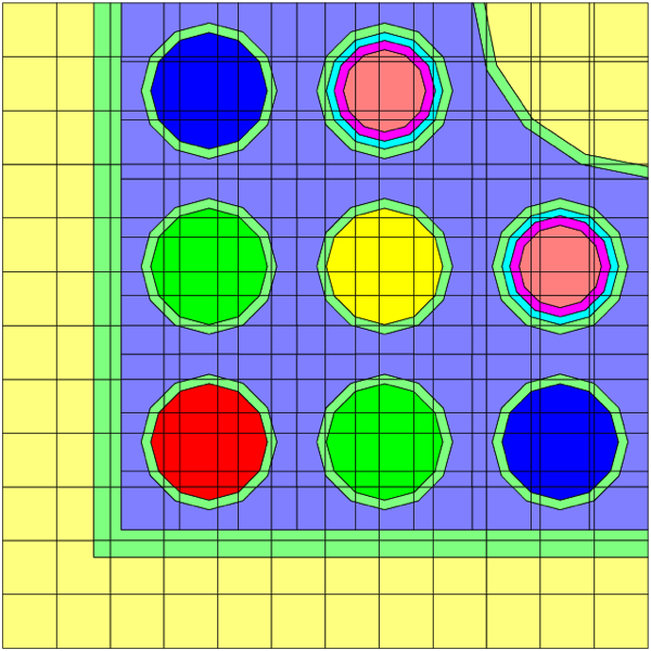
Fig. 3.1.12 BWR-like assembly design for triton8.

3.1.6.8. TRITON sample problem 10: triton10.inp

Sample problem triton10.inp performs NEWT-based depletion of a one-fourth symmetric assembly model. The primary intent of this sample problem is to test and to demonstrate the use of branches and archival of computed cross sections for a depletion case. The model includes two branch calculations-in addition to the nominal condition-that demonstrate the different perturbation outputs available in the BRANCH block. A two-group collapse is requested in the NEWT input, along with homogenization over all materials. (Note that the parameter specification parm=(addnux=1) is only used to reduce run-time of the sample problem.) At the end of the calculation, the binary file “xfile016” and text file “txtfile16” will exist in the temporary working directory and will contain all lattice physics parameters for all branches at all depletion states. These files are often copied back from the SCALE temporary working directory to another more permanent directory for subsequent post-processing.

' THIS SAMPLE PROBLEM TEST THE FOLLOWING:
'  ** t-depl sequence
'  ** v7-56 group library
'  ** centrm cross-section processing
'  ** latticecell cross-section processing option
'  ** deplete-by-constant power
'  ** parm=addnux=1 option to add 15 nuclides to fuel material
'  ** system power normalization
'  ** branch block to generate few-group cross-sections.
=t-depl parm=(addnux=1)
1/4 assembly model
v7-56
read comp
  uo2      1 0.95 923 92235 3.0 92238 97.0 end
  zirc2    2 1 595 end
  h2o      3 den=0.7135 1      579 end
  boron    3 den=0.7135 600e-6 579 end
  n        4 den=0.00125 1 595 end
  zirc2    5 1 579 end
  h2o      6 den=0.7135 1      579 end
  boron    6 den=0.7135 600e-6 579 end
  h2o      7 den=0.7135 1      579 end
  boron    7 den=0.7135 600e-6 579 end
  zirc2    8 1 579 end
  b4c      9 den=2.52 1 579 end
end comp
read celldata
  latticecell squarepitch pitch=1.4300 3 fueld=0.9294 1 gapd=0.9484  4 cladd=1.0719 2 end
end celldata
read depletion
  1
end depletion
read burndata
  power=40.0  burn=75 end
end burndata
read branch
  define fuel 1 end
  define mod  3 end
  define crout 8 9 end
  define crin  6 7 end
  define d2pset 10 1 0.53 end
  define d2pset 20 1 0.93 end
  tf=923 dm=.7135 tm=579 cr=0 sb=600 end
  dm=0.01 sb=0 d2p=20 end
  cr=1 d2p=10 tf=300 end
end branch
read model
1/4 assembly model
read parm
  echo=yes drawit=no cmfd=1 xycmfd=0 inners=2 epsilon=-5e-5 outers=300
end parm
read materials
  mix=1 pn=0 com="fuel"  end
  mix=2 pn=0 com="clad" end
  mix=3 pn=0 com="water" end
  mix=4 pn=0 com="gap" end
  mix=5 pn=0 com="guide tube" end
  mix=6 pn=0 com="CRout-clad" end
  mix=7 pn=0 com="CRout-abs" end
  mix=8 pn=0 com="CRin-clad" end
  mix=9 pn=0 com="CRin-abs" end
end materials
read geom
  unit 1
    com='fuel rod'
    cylinder 10 .4647
    cylinder 20 .4742
    cylinder 30 .53595
    cuboid   40  4p0.715
    media 1 1 10
    media 4 1 20 -10
    media 2 1 30 -20
    media 3 1 40 -30
    boundary  40 2 2
  unit 5
    com='guide tube'
    cylinder 10 .45
    cylinder 20 .52
    cylinder 30 .6502
    cylinder 40 .6934
    cuboid   50  4p0.715
    media 7 1 10
    media 6 1 20 -10
    media 3 1 30 -20
    media 5 1 40 -30
    media 3 1 50 -40
    boundary  50 2 2
  unit 11
    com='right half of fuel rod'
    cylinder 10 .4647   chord +x=0
    cylinder 20 .4742   chord +x=0
    cylinder 30 .53595  chord +x=0
    cuboid   40  0.715  0.0 2p0.715
    media 1 1 10
    media 4 1 20 -10
    media 2 1 30 -20
    media 3 1 40 -30
    boundary  40 1 2
  unit 12
    com='top half of fuel rod'
    cylinder 10 .4647   chord +y=0
    cylinder 20 .4742   chord +y=0
    cylinder 30 .53595  chord +y=0
    cuboid   40  2p0.715 0.715 0.0
    media 1 1 10
    media 4 1 20 -10
    media 2 1 30 -20
    media 3 1 40 -30
    boundary  40 2 1
  unit 51
    com='right half of guide tube'
    cylinder 10 .45   chord +x=0
    cylinder 20 .52   chord +x=0
    cylinder 30 .6502 chord +x=0
    cylinder 40 .6934 chord +x=0
    cuboid   50  0.715 0.0 2p0.715
    media 7 1 10
    media 6 1 20 -10
    media 3 1 30 -20
    media 5 1 40 -30
    media 3 1 50 -40
    boundary  50 1 2
  unit 52
    com='top half of guide tube'
    cylinder 10 .45   chord +y=0
    cylinder 20 .52   chord +y=0
    cylinder 30 .6502 chord +y=0
    cylinder 40 .6934 chord +y=0
    cuboid   50  2p0.715 0.715 0.0
    media 7 1 10
    media 6 1 20 -10
    media 3 1 30 -20
    media 5 1 40 -30
    media 3 1 50 -40
    boundary  50 2 1
  unit 53
    com='1/4 instrument tube'
    cylinder 10 .6502   chord +x=0 chord +y=0
    cylinder 20 .6934   chord +x=0 chord +y=0
    cuboid   40  0.715 0.0 0.715 0.0
    media 3 1 10
    media 5 1 20 -10
    media 3 1 40 -20
  boundary  40 1 1
global unit 10
    com='1/4 assembly'
    cuboid 10 10.725 0.0 10.725 0.0
    array 1 10 place 1 1 0 0
    media 3 1 10
  boundary 10 15 15
end geom
read coll
  40r1 16r2
end coll
read homog
  500 allmatl 1 2 3 4 5 6 7 8 9 end
end homog
read array
  ara=1 nux=8 nuy=8 typ=cuboidal pinpow=yes
  fill
    53  12 12 12 52 12 12 12
    11  1  1  1  1  1  1  1
    11  1  1  1  1  5  1  1
    11  1  1  5  1  1  1  1
    51  1  1  1  1  1  1  1
    11  1  5  1  1  5  1  1
    11  1  1  1  1  1  1  1
    11  1  1  1  1  1  1  1  end fill
end array
read bounds
  all=refl
end bounds
end model
end

3.1.6.9. TRITON sample problem 11: triton11.inp

Sample problem triton11.inp demonstrates the use of determining Dancoff factors for a BWR fuel assembly. The BWR assembly design contains a 7 $\times$ 7 array of fuel pins enclosed by a channel box (see Fig. 3.1.13). The in-channel moderator void fraction is 40%, and the bypass moderator void fraction is 0%. The input file contains an MCDANCOFF input file that calculates the Dancoff factors for each fuel pin (See the MCDANCOFF chapter). The MCDANCOFF input is essentially the equivalent of the KENO-VI model of the 2D assembly design. Following the MCDANCOFF input, the T-NEWT input is provided that shows how the computed Dancoff factors are inserted into the TRITON model. The Dancoff factors are inserted into the model via the centrmdata keyword entry in the CELLDATA block.

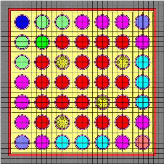
Fig. 3.1.13 triton11 BWR assembly design.

' THIS SAMPLE PROBLEM TESTS THE FOLLOWING:
'  ** mcdancoff sequence to compute problem dependent dancoffs.
=mcdancoff
PB CYCLE1
xn01
read comp
  uo2   1 den=10.42 0.99 900 92235 2.93 92234 0.0261 92236 0.0135 92238 97.0304 end
  uo2 201 den=10.42 0.99 900 92235 2.93 92234 0.0261 92236 0.0135 92238 97.0304 end
  uo2   2 den=10.42 0.99 900 92235 1.94 92234 0.0173 92236 0.0089 92238 98.0338 end
  uo2 202 den=10.42 0.99 900 92235 1.94 92234 0.0173 92236 0.0089 92238 98.0338 end
  uo2 212 den=10.42 0.99 900 92235 1.94 92234 0.0173 92236 0.0089 92238 98.0338 end
  uo2 203 den=10.42 0.99 900 92235 1.69 92234 0.0150 92236 0.0078 92238 98.2872 end
  uo2 213 den=10.42 0.99 900 92235 1.69 92234 0.0150 92236 0.0078 92238 98.2872 end
  uo2   4 den=10.42 0.99 900 92235 1.33 92234 0.0118 92236 0.0061 92238 98.6521 end
  uo2 500 den=10.29 0.97 900 92235 2.93 92234 0.0261 92236 0.0135 92238 97.0304 end
  gd2o3 500 den=10.29 0.03 900 end
  he 121 den=4.9559E-4 1 711.15 end
  zirc2 101 den=5.678 1 630 end
  h2o 111 den=0.4577 1 560 end
  zirc4 630 den=6.525 1 630 end
  h2o   620 den=0.738079 1 560  end
end comp
read parm
  gen=100 npg=100 nsk=0 htm=no flx=yes fdn=yes run=yes
end parm
read geom
  unit   11
    com="corner rod 1.33% enr"
    cylinder 1   0.60579  2p1.0
    cylinder 2   0.62103  2p1.0
    cylinder 3   0.71501  2p1.0
    cuboid   4 4p0.9375   2p1.0
    media   4 1 1
    media 121 1 2 -1
    media 101 1 3 -2
    media 111 1 4 -3
    boundary    4
  unit   12
    com="edge rod 1.69% enr"
    cylinder 1   0.60579  2p1.0
    cylinder 2   0.62103  2p1.0
    cylinder 3   0.71501  2p1.0
    cuboid   4 4p0.9375   2p1.0
    media 203 1 1
    media 121 1 2 -1
    media 101 1 3 -2
    media 111 1 4 -3
    boundary    4
  unit   14
    com="edge rod 1.94% enr"
    cylinder 1   0.60579  2p1.0
    cylinder 2   0.62103  2p1.0
    cylinder 3   0.71501  2p1.0
    cuboid   4 4p0.9375   2p1.0
    media 202 1 1
    media 121 1 2 -1
    media 101 1 3 -2
    media 111 1 4 -3
    boundary    4
  unit   17
    com="corner rod 1.69% enr"
    cylinder 1   0.60579  2p1.0
    cylinder 2   0.62103  2p1.0
    cylinder 3   0.71501  2p1.0
    cuboid   4 4p0.9375   2p1.0
    media 213 1 1
    media 121 1 2 -1
    media 101 1 3 -2
    media 111 1 4 -3
    boundary    4
  unit   22
    com="interior rod 1.94% enr"
    cylinder 1   0.60579  2p1.0
    cylinder 2   0.62103  2p1.0
    cylinder 3   0.71501  2p1.0
    cuboid   4 4p0.9375   2p1.0
    media   2 1 1
    media 121 1 2 -1
    media 101 1 3 -2
    media 111 1 4 -3
    boundary    4
  unit   23
    com="interior rod 2.93% enr"
    cylinder 1   0.60579  2p1.0
    cylinder 2   0.62103  2p1.0
    cylinder 3   0.71501  2p1.0
    cuboid   4 4p0.9375   2p1.0
    media   1 1 1
    media 121 1 2 -1
    media 101 1 3 -2
    media 111 1 4 -3
    boundary    4
  unit   33
    com="interior gad pin"
    cylinder 5   0.60579  2p1.0
    cylinder 6   0.62103  2p1.0
    cylinder 7   0.71501  2p1.0
    cuboid   8 4p0.9375   2p1.0
    media 500 1 5
    media 121 1 6 -5
    media 101 1 7 -6
    media 111 1 8 -7
    boundary    8
  unit   37
    com="edge rod 2.93% enr"
    cylinder 1   0.60579  2p1.0
    cylinder 2   0.62103  2p1.0
    cylinder 3   0.71501  2p1.0
    cuboid   4 4p0.9375   2p1.0
    media 201 1 1
    media 121 1 2 -1
    media 101 1 3 -2
    media 111 1 4 -3
    boundary    4
  unit   77
   com="corner rod 1.94% enr"
    cylinder 1   0.60579  2p1.0
    cylinder 2   0.62103  2p1.0
    cylinder 3   0.71501  2p1.0
    cuboid   4 4p0.9375   2p1.0
    media 212 1 1
    media 121 1 2 -1
    media 101 1 3 -2
    media 111 1 4 -3
    boundary    4
global unit 100
    cuboid  1   4p6.5625   2p1.0
    array 1 1  place 4 4 1  0.0 0.0 0.0
    cuboid  2   4p6.70306  2p1.0
    cuboid  3   4p6.90626  2p1.0
    cuboid  10  4p7.62     2p1.0
    media   111 1 2 -1
    media   630 1 3 -2
    media   620 1 10 -3
    boundary 10
end geom

read array
  ara=1 nux=7 nuy=7 nuz=1 typ=cuboidal
  fill
    17  14  37  37  37  14  77
    14  23  33  23  23  23  14
    14  23  23  23  33  23  37
    14  23  23  23  23  23  37
    12  23  33  23  23  33  37
    12  22  23  23  23  23  14
    11  12  12  14  14  14  17 end fill
end array
read bounds
  all=refl
end bounds
read start
  dancoff  array  1  1  1  1  unit  17  region 1
  dancoff  array  1  1  2  1  unit  14  region 1
  dancoff  array  1  1  3  1  unit  14  region 1
  dancoff  array  1  1  4  1  unit  14  region 1
  dancoff  array  1  1  5  1  unit  12  region 1
  dancoff  array  1  1  6  1  unit  12  region 1
  dancoff  array  1  1  7  1  unit  11  region 1
  dancoff  array  1  2  1  1  unit  14  region 1
  dancoff  array  1  2  2  1  unit  23  region 1
  dancoff  array  1  2  3  1  unit  23  region 1
  dancoff  array  1  2  4  1  unit  23  region 1
  dancoff  array  1  2  5  1  unit  23  region 1
  dancoff  array  1  2  6  1  unit  22  region 1
  dancoff  array  1  3  1  1  unit  37  region 1
  dancoff  array  1  3  2  1  unit  33  region 1
  dancoff  array  1  3  3  1  unit  23  region 1
  dancoff  array  1  3  4  1  unit  23  region 1
  dancoff  array  1  3  5  1  unit  33  region 1
  dancoff  array  1  4  1  1  unit  37  region 1
  dancoff  array  1  4  2  1  unit  23  region 1
  dancoff  array  1  4  3  1  unit  23  region 1
  dancoff  array  1  4  4  1  unit  23  region 1
  dancoff  array  1  5  1  1  unit  37  region 1
  dancoff  array  1  5  2  1  unit  23  region 1
  dancoff  array  1  5  3  1  unit  33  region 1
  dancoff  array  1  6  1  1  unit  14  region 1
  dancoff  array  1  6  2  1  unit  23  region 1
  dancoff  array  1  7  1  1  unit  77  region 1
end start
end data
end

3.1.6.10. TRITON sample problem 12: triton12.inp

Sample problem triton12.inp illustrates the use of the TRITON-NEWT with a model with numerous mixtures and aliases. Sample problem 11 demonstrates how MCDANCOFF is used to compute fuel pin Dancoff factors for designs where nonuniform lattice effects play a critical role in cross section processing. The Dancoff factors are inserted into the follow-on T-NEWT model through the centrmdata keyword in the CELLDATA block. The output for the T-NEWT model in sample problem 11 provides an adjusted moderator pitch needed to preserve the user-specified Dancoff factor. As common in other sample problems, several input options were used to reduce the run-time—and therefore solution accuracy—of the sample problem.

=t-newt   parm=(check)
PB CYCLE1
v7-252
' Data taken from:
'        Benchmark for Uncertainty Analysis in Modeling (UAM)
'        for Design, Operation and Safety Analyses of LWRs,
'        Nuclear Energy Agency, 2007.
read alias
 $gadpin 500 end
 $clad   101 102 103 104 105 301 302 303 304 305 end
 $mod    111 112 113 114 115 311 312 313 314 315 end
 $gap    121 122 123 124 125 321 322 323 324 325 end
end alias
read comp
' 2.93% enriched fuel pin
  uo2   1 den=10.42 0.99 900 92235 2.93 92234 0.0261 92236 0.0135 92238 97.0304 end
  uo2 201 den=10.42 0.99 900 92235 2.93 92234 0.0261 92236 0.0135 92238 97.0304 end
' 1.94% enriched fuel pin
  uo2   2 den=10.42 0.99 900 92235 1.94 92234 0.0173 92236 0.0089 92238 98.0338 end
  uo2 202 den=10.42 0.99 900 92235 1.94 92234 0.0173 92236 0.0089 92238 98.0338 end
  uo2 212 den=10.42 0.99 900 92235 1.94 92234 0.0173 92236 0.0089 92238 98.0338 end
' 1.69% enriched fuel pin
  uo2 203 den=10.42 0.99 900 92235 1.69 92234 0.0150 92236 0.0078 92238 98.2872 end
  uo2 213 den=10.42 0.99 900 92235 1.69 92234 0.0150 92236 0.0078 92238 98.2872 end
' 1.33% enriched fuel pin
  uo2   4 den=10.42 0.99 900 92235 1.33 92234 0.0118 92236 0.0061 92238 98.6521 end
' 3% Gd2O3 by weigh, 2.93% enriched fuel pin
  uo2   $gadpin den=10.29 0.97 900 92235 2.93 92234 0.0261 92236 0.0135 92238 97.0304 end
  gd2o3 $gadpin den=10.29 0.03 900 end
' gap/clad/moderator
  he    $gap  den=4.9559E-4 1 711.15  end
  zirc2 $clad den=5.678 1 630 end
  h2o   $mod    den=0.4577 1  560  end
' channel
  zirc4 630 den=6.525 1 630 end
' water in bypass
  h2o   620 den=0.738079 1 560  end
end comp
read celldata
  latticecell squarep pitch=1.87452 111 fuelr=0.60579   1 gapr=0.62103 121 cladr=0.71501 101 end
    centrmdata dan2pitch=0.504 end centrmdata
  latticecell squarep pitch=1.87452 112 fuelr=0.60579   2 gapr=0.62103 122 cladr=0.71501 102 end
    centrmdata dan2pitch=0.494 end centrmdata
  latticecell squarep pitch=1.87452 114 fuelr=0.60579   4 gapr=0.62103 124 cladr=0.71501 104 end
    centrmdata dan2pitch=0.362 end centrmdata
  latticecell squarep pitch=1.87452 311 fuelr=0.60579 201 gapr=0.62103 321 cladr=0.71501 301 end
    centrmdata dan2pitch=0.423 end centrmdata
  latticecell squarep pitch=1.87452 312 fuelr=0.60579 202 gapr=0.62103 322 cladr=0.71501 302 end
    centrmdata dan2pitch=0.423 end centrmdata
  latticecell squarep pitch=1.87452 313 fuelr=0.60579 203 gapr=0.62103 323 cladr=0.71501 303 end
    centrmdata dan2pitch=0.417 end centrmdata
  latticecell squarep pitch=1.87452 314 fuelr=0.60579 212 gapr=0.62103 324 cladr=0.71501 304 end
    centrmdata dan2pitch=0.359 end centrmdata
  latticecell squarep pitch=1.87452 315 fuelr=0.60579 213 gapr=0.62103 325 cladr=0.71501 305 end
    centrmdata dan2pitch=0.357 end centrmdata
  latticecell squarep pitch=1.87452 115 fuelr=0.60579 500 gapr=0.62103 125 cladr=0.71501 105 end
    centrmdata dan2pitch=0.506 end centrmdata
end celldata

read model
PB CYCLE1
read parm
 echo=yes timed=yes drawit=yes cmfd=1 epsilon=3e-3 inners=2 therm=yes therms=1 outers=9999 xycmfd=4
end parm
read materials
  mix=  1        pn=1  com='2.93% UO2'         end
  mix=  2        pn=1  com='1.94% UO2'         end
  mix=  4        pn=1  com='1.33% UO2'         end
  mix=$gadpin    pn=1  com='2.93% UO2 (3% Gd)' end
  mix=201        pn=1  com='2.93% UO2, edge'   end
  mix=202        pn=1  com='1.94% UO2, edge'   end
  mix=212        pn=1  com='1.94% UO2, corner' end
  mix=203        pn=1  com='1.69% UO2, edge'   end
  mix=213        pn=1  com='1.69% UO2, corner' end
  mix=111        pn=2  com='H2O(void)'         end
  mix=101        pn=1  com='Zirc2'             end
  mix=121        pn=1  com='Helium'            end
  mix=620        pn=2  com='H2O(solid)'        end
  mix=630        pn=1  com='Zirc4'             end
end materials
read geom
  unit   11
    com="corner rod 1.33% enr"
    cylinder 1   0.60579
    cylinder 2   0.62103
    cylinder 3   0.71501
    cuboid   4 4p0.9375
    media   4 1 1
    media 121 1 2 -1
    media 101 1 3 -2
    media 111 1 4 -3
    boundary    4  2 2
  unit   12
    com="edge rod 1.69% enr"
    cylinder 1   0.60579
    cylinder 2   0.62103
    cylinder 3   0.71501
    cuboid   4 4p0.9375
    media 203 1 1
    media 121 1 2 -1
    media 101 1 3 -2
    media 111 1 4 -3
    boundary    4  2 2
  unit   14
    com="edge rod 1.94% enr"
    cylinder 1   0.60579
    cylinder 2   0.62103
    cylinder 3   0.71501
    cuboid   4 4p0.9375
    media 202 1 1
    media 121 1 2 -1
    media 101 1 3 -2
    media 111 1 4 -3
    boundary    4  2 2
  unit   17
    com="corner rod 1.69% enr"
    cylinder 1   0.60579
    cylinder 2   0.62103
    cylinder 3   0.71501
    cuboid   4 4p0.9375
    media 213 1 1
    media 121 1 2 -1
    media 101 1 3 -2
    media 111 1 4 -3
    boundary    4  2 2
  unit   22
    com="interior rod 1.94% enr"
    cylinder 1   0.60579
    cylinder 2   0.62103
    cylinder 3   0.71501
    cuboid   4 4p0.9375
    media   2 1 1
    media 121 1 2 -1
    media 101 1 3 -2
    media 111 1 4 -3
    boundary    4  2 2
  unit   23
    com="interior rod 2.93% enr"
    cylinder 1   0.60579
    cylinder 2   0.62103
    cylinder 3   0.71501
    cuboid   4 4p0.9375
    media   1 1 1
    media 121 1 2 -1
    media 101 1 3 -2
    media 111 1 4 -3
    boundary    4  2 2
  unit   33
    com="interior gad pin"
    cylinder 1   0.270917524
    cylinder 2   0.383135237
    cylinder 3   0.469242916
    cylinder 4   0.541835048
    cylinder 5   0.60579
    cylinder 6   0.62103
    cylinder 7   0.71501
    cuboid   8 4p0.9375
    media 500 1 1
    media 500 1 2 -1
    media 500 1 3 -2
    media 500 1 4 -3
    media 500 1 5 -4
    media 121 1 6 -5
    media 101 1 7 -6
    media 111 1 8 -7
    boundary    8  2 2
  unit   37
    com="edge rod 2.93% enr"
    cylinder 1   0.60579
    cylinder 2   0.62103
    cylinder 3   0.71501
    cuboid   4 4p0.9375
    media 201 1 1
    media 121 1 2 -1
    media 101 1 3 -2
    media 111 1 4 -3
    boundary    4  2 2
  unit   77
   com="corner rod 1.94% enr"
    cylinder 1   0.60579
    cylinder 2   0.62103
    cylinder 3   0.71501
    cuboid   4 4p0.9375
    media 212 1 1
    media 121 1 2 -1
    media 101 1 3 -2
    media 111 1 4 -3
    boundary    4  2 2
global unit 100
   cuboid  1   4p6.70306
   array 1 1  place 4 4  0.0 0.0
   cuboid  2   4p6.90626
   cuboid  10  4p7.62
   media   111 1 1
   media   630 1 2 -1
   media   620 1 10 -2
   boundary 10 32 32
end geom
read array
  ara=1 nux=7 nuy=7 typ=cuboidal
  fill
    17  14  37  37  37  14  77
    14  23  33  23  23  23  14
    14  23  23  23  33  23  37
    14  23  23  23  23  23  37
    12  23  33  23  23  33  37
    12  22  23  23  23  23  14
    11  12  12  14  14  14  17 end fill
end array
read bounds
  all=refl
end bounds
end model
end

3.1.6.11. TRITON6 sample problem 1: triton6-1.inp

Sample problem triton6-1.inp is an example of KENO-VI-based depletion for an infinite lattice of cylinders fabricated with particulate TRISO fuel dispersed in a graphite matrix. This provides an example of the cross section processing specification of a doubly heterogeneous (DOUBLEHET) media and use of the resultant homogenized media in a depletion calculation.

' THIS SAMPLE PROBLEM TEST THE FOLLOWING:
'  ** t6-depl sequence
'  ** v7-252 group library
'  ** centrm cross section processing
'  ** double-heterogeneous cross section processing option
'  ** deplete-by-constant power and flux
'  ** system power normalization
=t6-depl      parm=centrm
Test case - infinite cylinder
v7-252
read comp
' fuel kernel
  u-238  101 0 1.72877e-2 293.6 end
  u-235  101 0 5.92585e-3 293.6 end
  o      101 0 4.64272e-2 293.6 end
  b-10   101 0 1.14694e-7 293.6 end
  b-11   101 0 4.64570e-7 293.6 end
' first coating
  c      102 0 5.26449e-2 293.6 end
' inner pyro carbon
  c      103 0 9.52621e-2 293.6 end
' silicon carbide
  c      104 0 4.77240e-2 293.6 end
  si     104 0 4.77240e-2 293.6 end
' outer pyro carbon
  c      105 0 9.52621e-2 293.6 end
' graphite matrix
  c      106 0 8.77414e-2 293.6 end
' carbon pebble outer coating
  c      107 0 8.77414e-2 293.6 end
  b-10   107 0 9.64977e-9 293.6 end
  b-11   107 0 3.90864e-8 293.6 end
  he-3    108 0 3.71220e-11 293.6 end
  he-4    108 0 2.65156e-5 293.6 end
end comp

read celldata
  doublehet  right_bdy=white fuelmix=10 end
    gfr=0.025    101
    coatt=0.009  102
    coatt=0.004  103
    coatt=0.0035 104
    coatt=0.004  105
    matrix=106 numpar=15000 end grain
  rod squarepitch right_bdy=white hpitch=3.0 108 fuelr=2.5 cladr=3.0 107 fuelh=365 end
end celldata
read depletion
  101 flux 107
end depletion
read burndata
  power=30 burn=600 down=30 nlib=1 end
end burndata
read model
read param
  npg=200 gen=350 nsk=100 htm=no
end param
read geometry
  global unit 1
    cylinder 1 2.5 99 -99
    cylinder 2 3.0 99 -99
    cuboid   3 4p3.0 99 -99
    media    10    1       1
    media     107    1       2  -1
    media     108    1       3  -2
  boundary     3
end geometry
read bounds
  all=mirror
end bounds
end data
end model
end

References

TRITONBPBR17: B. R. Betzler, J. J. Powers, N. R. Brown, and B. T. Rearden. Molten Salt Reactor Tools in SCALE. In ANS Mathematics & Computation Topical Meeting, Apr. 16–20. Jeju, Korea, 2017.
TRITONBPW17: B. R. Betzler, J. J. Powers, and A. Worrall. Molten salt reactor neutronics and fuel cycle modeling and simulation with scale. Annals of Nuclear Energy, 101:489–503, 2017. doi:10.1016/j.anucene.2016.11.040.
TRITONDB11: M.D. DeHart and S. M. Bowman. Reactor physics methods and analysis capabilities in scale. Nuclear Technology, 174(2):196–213, 2011. doi:10.13182/NT174-196.
TRITONVBWF20: P. V. Vicente, B. R. Betzler, W. A. Wieselquist, and M. Fratoni. Modeling Molten Salt Reactor Fission Product Removal with SCALE. Technical Report ORNL/TM-2019/1418, Oak Ridge National Laboratory, Oak Ridge, TN (USA), 2020.

3.1. TRITON: A Multipurpose Transport, Depletion, And Sensitivity and Uncertainty Analysis Module

3.1.1. Acknowledgments

3.1.2. Introduction

3.1.2.1. TRITON Sequences

3.1.2.1.1. Cross section processing sequence (T-XSEC)

3.1.2.1.2. Transport sequences (T-XSDRN, T-NEWT)

3.1.2.1.3. Depletion sequences (T-DEPL, T-DEPL-1D, T5-DEPL, T6-DEPL, T5-DEPL-SHIFT, T6-DEPL-SHIFT)

3.1.2.2. Predictor-corrector depletion process

3.1.2.3. Data resources

3.1.2.4. Lattice physics analysis

3.1.3. Input Description

3.1.3.1. Cross section processing

3.1.3.1.1. Combined two-region and SN cross section processing

3.1.3.1.2. User-defined Dancoff factors

3.1.3.2. Transport sequences

3.1.3.3. Depletion sequences input

3.1.3.3.1. BURNDATA block

3.1.3.3.2. BRANCH block

3.1.3.3.3. BRANCH block with user-defined Dancoff factors

3.1.3.3.4. DEPLETION block

3.1.3.3.4.1. Basic DEPLETION block format

3.1.3.3.4.2. ORIGEN depletion options

3.1.3.3.4.3. Cross section processing simplification using ASSIGN

3.1.3.3.5. TIMETABLE block

3.1.3.3.5.1. Temperature and density

3.1.3.3.5.2. Material swap

3.1.3.3.5.3. Material flow

3.1.3.3.6. OPUS block

3.1.3.3.6.1. Selection of materials for OPUS processing

3.1.3.3.6.2. Specification of stacked OPUS cases

3.1.3.3.7. TALLIES and DEFINITIONS block

3.1.3.4. ALIAS block

3.1.3.4.1. COMPOSITION block aliases

3.1.3.4.2. CELLDATA block aliases

3.1.3.4.3. DEPLETION block aliases

3.1.3.4.4. TIMETABLE block aliases

3.1.3.4.5. BRANCH block aliases

3.1.3.4.6. NEWT MATERIAL block aliases

3.1.3.4.7. KEEP_OUTPUT block

3.1.3.5. TRITON control parameters

3.1.3.5.1. Check mode: parm=check

3.1.3.5.2. Multigroup cross section processing options

3.1.3.5.3. Creating a broad group library: parm=weight, parm=(weight=N)

3.1.3.5.4. Inclusion of additional nuclides for depletion: parm=(addnux=N)

3.1.3.5.5. Few-group reaction cross section calculation control for continuous energy depletion: parm=(cxm=N)

3.1.3.5.6. Infinite dilution cutoff control: parm=(infdcutoff=X)

3.1.3.5.7. Override of the maximum number of days per depletion subinterval: PARM=(MAXDAYS=N)

3.1.4. Output Files Created by TRITON

3.1.4.1. Standard composition restart files

3.1.4.2. Lattice physics parameters

3.1.4.3. ORIGEN binary library files (.f33)

3.1.4.4. ORIGEN binary concentration file (.f71)

3.1.4.5. Binary mesh response files (.3dmap)

3.1.4.6. Nubar files (.txt)

3.1.4.7. Binary Shift output file (.h5)

3.1.5. Output Description

3.1.5.1. Control parameter edit

3.1.5.2. T-XSEC output

3.1.5.3. T-NEWT and T-XSDRN output

3.1.5.4. Depletion sequence output

3.1.5.4.1. Burnup history summary (all depletion sequences)

3.1.5.4.2. Embedded transport model output

3.1.5.4.3. System mass balance table

3.1.5.4.4. Power balance tables

3.1.5.4.4.1. ORIGEN binary concentration file listing

3.1.6. TRITON Sample Cases

3.1.6.1. TRITON sample problem 1: triton1.inp

3.1.6.2. TRITON sample problem 2: triton2.inp

3.1.6.3. TRITON sample problem 3: triton3.inp

3.1.6.3.1. TRITON sample problem 4: triton4.inp

3.1.6.4. TRITON sample problem 5: triton5.inp

3.1.6.5. TRITON sample problem 6: triton6.inp

3.1.6.6. TRITON sample problem 7: triton7.inp

3.1.6.7. TRITON sample problem 8: triton8.inp

3.1.6.8. TRITON sample problem 10: triton10.inp

3.1.6.9. TRITON sample problem 11: triton11.inp

3.1.6.10. TRITON sample problem 12: triton12.inp

3.1.6.11. TRITON6 sample problem 1: triton6-1.inp

3.1.7. Appendices

3.1.3.1.1. Combined two-region and S_N cross section processing