3.2. POLARIS - 2D Light Water Reactor Lattice Physics Module

Code Responsible(s): M. A. Jessee Contributors: M. A. Jessee, W. A. Wieselquist, A. M. Holcomb, S. W. Hart, J. W. Bae, K. S. Kim, C. A. Gentry, S. E. Skutnik, U. Mertyurek, J. Yang

ABSTRACT

Polaris is an easy-to-use light water reactor (LWR) lattice physics capability for SCALE. Originally released in SCALE 6.2, Polaris uses the Embedded Self Shielding Method (ESSM) for multigroup cross section processing and a transport solver based on the Method of Characteristics (MOC). The ESSM computes multigroup self-shielded cross sections using Bondarenko interpolation methods. The background cross section used in the interpolation is determined by iterative 2D MOC fixed-source transport calculations. Polaris is integrated with ORIGEN for depletion calculations. Each pin-or each radial subregion of the pin-is depleted based on the local power distribution. An optional critical spectrum calculation is incorporated into the depletion calculation and the output edits of few-group homogenized cross sections. Few-group cross sections are archived to the lattice physics archive (.t16 and .x16 extension) file, which can be used in subsequent core simulator calculations. Nuclide inventories are archived to the ORIGEN binary concentration file (.f71 extension), which can be used in subsequent SCALE calculations for source term characterization or radition shielding. Depletion and decay data are archived to the ORIGEN binary library file (.f33 extension), and can also be used in subsequent source term calculations.

ACKNOWLEDGMENTS

The authors express gratitude to the U.S. Nuclear Regulatory Commission (NRC) for funding Polaris development. The author acknowledges D. Algama (former NRC), A. Bielen, L. Kyriazidis, and H. Esmaili for their support of the project.

3.2.1. Introduction

Polaris was introduced in SCALE 6.2 to provide 2D lattice physics analysis capability for light water reactor (LWR) fuel designs. For multigroup cross section processing, Polaris uses the Embedded Self-Shielding Method (ESSM) [POLARISWK12]. Unlike SCALE multigroup sequences that use XSProc, ESSM does not require user-defined unit cell definitions. ESSM computes multigroup cross sections using Bondarenko interpolation methods. The background cross section used in the interpolation is determined by iterative 2D fixed source transport calculations. Both the ESSM fixed-source calculations and the keff calculation utilize a Method of Characteristics (MoC) transport solver developed in the Exnihilo computational package.

Polaris is integrated with ORIGEN for depletion calculations. Each pin-or each radial subregion of the pin-is depleted based on the local power distribution. An optional critical spectrum calculation is incorporated into the depletion calculation for computing depletion reaction rates and/or few-group homogenized cross sections. A complete description of the Polaris computational methods is provided in [POLARISJWM+21].

Polaris provides an easy-to-use input format to allow users to set up lattice models with minimal lines of input. All recognized Polaris commands are shown in Table 3.2.1. Note that many commands support short and long forms. The allowed basic Types for input are described in Table 3.2.2. The special Polaris TYPES are shown in Table 3.2.3. The convention used in this manual is that basic types appear italicized and capitalized (Type), while special Polaris types appear in all caps (TYPE).

Table 3.2.1 Polaris commands.
card	long command	short command(s)
system	system	sys
geometry	geometry	geom
composition	composition	comp
property	property	prop
material	material	mat
burnup	bu or dbu	-
power	power	pow
options	option	opt
time	t or dt	-
state	state	-
branch block	branch	-
pin geometry component	pin	-
assembly pin map	pinmap	-
assembly channel	channel	-
assembly half gap	hgap	-
channel box	box	-
shield	shield	-
deplete	deplete	-
slab geometry component	slab	-
power basis materials	basis	-
assembly inserts	insert	-
assembly control elements water cross geometry displacement maps spatial meshing detector tallies operating histories restart cumulative burnup	control cross dxmap (dymap) mesh detector history bui (ti)	- - - - - - -

Table 3.2.2 Basic Types in Polaris input.
basic type	description	examples	incorrect examples
Word	starts with a character A-Z or a-z and includes characters, numbers, underscores	uox bor_water_500ppm FUEL	uox_enr5.1 316SS uox-3.1
Int	integer	17 92235 2 565	31.4 uox
Bool	boolean/logical	yes false	TRUE No
Real	any number	565 10.257 1.5e-6	yes bor_water
String	a single or double quoted string	“INFMED” “Includes spaces” ‘NONE’	Includes spaces
Value	any non-word		Int\|Bool\|Real\| String

Table 3.2.3 Special Polaris Types.
Polaris type	description	variants
STYPE	system type	PWR \| BWR
GTYPE	geometry type	ASSM \| REFL
CTYPE	composition type	NUM \| WT \| FORM \| CONC \| LW \| UOX \| ENRU \| UN \| USI
PTYPE	property type	SOLP \| DOPANT
ETYPE	control element type	RODLET\|BLADE
OTYPE	option type	KEFF \| BOND \| ESSM \| CRITS PEC \| FG \| DEPL \| RUN \| PRINT \| GAMMA \| GEOM \| DATA

The Polaris input supports a very flexible input scheme that allows some elements to be suppressed for better readability. With key=value type input, when the standard order of keys is used, the keys may be suppressed. Consider the following input specification as an example.

geometry GNAME : ASSM npins=Int ppitch=Real [sym=<FULL>|SE]

The geometry card requires a geometry name (GNAME) in the first group, then a geometry type (GTYPE) which is ASSM here indicating an assembly geometry. The remaining arguments have keys: “npins” with an integer value, “ppitch” with a real value, and the optional “sym” with either FULL or SE values (optional arguments are always shown in square brackets: [sym=<FULL>|SE]. The default value is in angle brackets: <FULL>. The pipe “|” shows an or relation (i.e., FULL or SE is an acceptable value). With the flexible input processing, the following inputs are all valid and identical.

geometry FuelNode : ASSM npins=15 ppitch=1.43 sym=FULL
geometry FuelNode : ASSM 15 1.43 FULL
geometry FuelNode : ASSM sym=FULL ppitch=1.43 npins=15
geometry FuelNode : ASSM 15 1.43
geometry FuelNode ASSM 15 1.43

The group separator “:” is suppressed in the last variant. This is possible in any situation where (1) the group is implicitly terminated by running out of arguments or (2) the next type does not match the expected type in the current group. For example, consider the hgap card:

hgap [ d ] [: M ]

In this card, d and M are values (without keys) defined as Real and material name (MNAME), respectively. The following form would automatically bypass the Real value, which allows a default, and set the interassembly gap material name as COOL.2.

hgap COOL.2

3.2.2. SCALE 6.3 Polaris Input Updates

For the release of SCALE 6.2.3, several new input cards were implemented into Polaris to model boiling water reactor (BWR) geometries and neutron/gamma detectors, which requires a gamma transport calculation. Moreover, improvements to existing input cards were implemented, along with the ability to specify time-dependent state properties and the ability to specify one or more depletion histories. This section describes the new and modified input cards that are included in the Polaris input format for SCALE 6.3, which are accessible as part of the release of SCALE 6.2.3.

To maximize backwards compatibility for input files developed with the original SCALE 6.2.0 release, the new and modified input cards are not available by default with SCALE 6.2.3. The new and modified input cards were activated if the input file begins with =polaris_6.3 rather than =polaris. The suffix “_6.3” is an indicator to the Polaris input processor to use the SCALE 6.3 input format. For the SCALE 6.3 release, the original input cards supported in the SCALE 6.2 input format will be available if the input file begins with =polaris_6.2, with the new SCALE 6.3 defaults being used for inputs with =polaris.

The new input cards to model BWR geometries include:

cross – define the interior water cross geometry of SVEA assembly designs;
dxmap (or dymap) – define displacement maps that indicate that translation of the pin center in the x- (or y-) direction;
control <BLADE> – define the control blade geometry;
mesh – define advanced spatial meshing options for different materials; and
option <GEOM> – define geometry tolerances, advance meshing options, and plotting options.

The modified input cards to model BWR geometries include:

pin – define circular and square-based geometry zones, as well as arbitrarily sized pins, e.g. size=1.5 water rod in some 9x9 BWR lattice designs; and
box – define channel box geometry with arbitrary number of zones and cutout regions.

For neutron/gamma detector modeling, there is a new detector card and an addition to the existing option <FG> card to enable output to the few-group cross section output (T16) file.

To control the gamma calculation, an option <GAMMA> has been added.

The new input cards for time-dependent modeling include:

history – define one or more operating histories in the input file; and
bui (or ti) – define restart cumulative burnup (or time) values.

The modified input cards for time-dependent modeling include:

state – define one or more time-independent or time-dependent state properties;
bu (or t) – define cumulative burnup (or time) values; and
dbu (or dt) – define incremental burnup (or time) values.

Example input files are included in the ${SCALE}/regression/input directory:

polaris.6.3.atrium9x9.inp and polaris.6.3.atrium10x10.inp – prototypic ATRIUM models;
polaris.6.3.blade1.inp and polaris.6.3.blade2.inp – control <BLADE> examples;
polaris.6.3.ge7x7.inp through polaris.6.3.ge10x10.inp – prototypic GE models;
polaris.6.3.svea100.inp and polaris.6.3.svea64.inp – prototypic SVEA models; and
polarisHistory.inp: history example.

3.2.3. Setup

The cards in this section generally appear at the beginning of an input file. Note that the manual is organized with each card starting a new page. This is especially convenient when printing a few cards across different sections.

3.2.3.1. title - case title lines

title Line₁ Line₂ … Line_i … Line_N

param	type	name	details	default
Line_i	String	line	used in output file headers	“DEFAULT TITLE”

Examples:

title "Westinghouse 15x15"

title "Westinghouse 15x15"
        "Condition: Hot Full Power"
        "Date: 10/18/2012"

Comments:

The title card gives a title to this Polaris case, which appears as a descriptive header on the output file. The additional lines may be used to document a subcase or to embed additional information in the output file in an orderly way (e.g., author, date, project identifier).

The title card is optional.

See also:

lib

3.2.3.2. library - nuclear data libraries

lib [mg=*String*]

param	type	name	details	default
mg	String	multigroup library	multigroup cross section library	“fine_n”

Examples:

% a name of library in the DATA directory
% use SCALE 252g ENDF/B-VII.1 library
lib "fine_therm"   % Alias for the V7.1 252g-neutron 47g-gamma library

% use SCALE 56g ENDF/B-VII.1 library
lib mg="broad_lwr"   % Alias for the V7.1 56g-neutron 19g-gamma library

% a name of a local library in the temporary working directory
% (useful in SAMPLER calculations)
lib "perturbed_xs_library"

% fully specified path
lib "C:\scale6.3\data\scale.rev05.xn252v7.1"

Comments:

The lib card specifies the multigroup library location. See SCALE’s FileNameAliases.txt file in the installation directory for up-to-date library aliases for the fine and broad group libraries provided in SCALE’s data directory. Only the 252-group and the 56-group cross section libraries are recommended to be used in Polaris. Full specification of the file path is acceptable, as in the final example shown above.

The lib card is optional.

See also:

title

3.2.4. Geometry

The highest level structures in the model are named and defined with a geometry card. The general outline for a geometry definition is shown below. Two types of geometry are currently supported, ASSM for pressurized water reactor (PWR) or boiling water reactor (BWR) assemblies with fuel elements in a square-pitch, and REFL for an assembly-adjacent reflector.

geom GNAME : GTYPE arguments

param	type	name	details	default
GNAME	Word	geometry name
GTYPE	-	geometry type
	ASSM	assembly	see pin & pinmap
	REFL	reflector	see slab
arguments	-	remaining arguments	depends on GTYPE

The control element geometry is also enumerated with types, as shown below. To model PWR-type rod cluster control assemblies (RCCAs), the RODLET element type is used in conjunction with pin definitions. In future releases of Polaris, other control element types, such as BWR-type control blades will be supported..

control INAME : ETYPE arguments

param	type	name	details	default
INAME	Word	control element name
ETYPE	-	control element type
	RODLET	PWR-type RCCA	requires PINIDs
arguments	-	remaining arguments	depends on ETYPE

3.2.4.1. geometry<ASSM> – assembly

geom GNAME : ASSM

npins=Int
ppitch=Real
[sym=<FULL>|SE]
[modular=*Bool*]

param	type	name	details	default
GNAME	Word	assembly name
GTYPE	ASSM
npins	Int	number of pins	on each side of the assembly
ppitch	Real	pin pitch	units: cm
sym	FULL\|SE	symmetry	assembly symmetry, FULL: no symmetry, SE: south-east quarter	FULL
modular	Bool	modular option	True: modular geometry False: standard geometry Requires sym=FULL	False

Examples:

% simple pincell
geom MyPin : ASSM 1 1.5

% 17x17 Westinghouse with 1.26 cm pin pitch in quarter symmetry
geom FuelNode : ASSM 17 1.26 sym=SE

Comments:

Examples:

% simple pincell

geom MyPin : ASSM 1 1.5

% 17x17 Westinghouse with 1.26 cm pin pitch in quarter symmetry

geom FuelNode : ASSM 17 1.26 sym=SE

% Large 200x200 map of pins using modular option

geom FuelNode : ASSM 200 1.5 sym=FULL modular=True

Comments:

The assembly geometry describes the basic elements of an assembly. The pin and pinmap cards are required to finalize the assembly geometry. The hgap card specifies the interassembly half gap, and the channel specifies the channel material for the assembly.

The modular option is useful for large arrays of pins—for example, critical benchmarks such as KRITZ, DIMPLE, BW 1810. This option should be used only for problems >35 pins per side, FULL symmetry only, and without interassembly gaps or channel boxes. The modular option is set to False (or no) by default.

See also:

pinmap, pin, hgap, box, channel, control, insert

3.2.4.2. geometry<REFL> - reflector

geom GNAME : REFL

thick=REAL

param	type	name	details	default
GNAME	Word	reflector name
GTYPE	REFL
thick	Real	thickness	units: cm

Examples:

% defines a 20 cm reflector
geom ReflectorNode : REFL 20.0

Comments:

The reflector geometry describes the basic elements of a simple slab-type reflector. The slab card can be used to define geometric dimensions and mesh for the reflector geometry.

See also:

slab

3.2.4.3. channel - coolant channel

channel [M_chan =MCLASS]

param	type	name	details	default
M_chan	MCLASS	material class	initializes materials in outermost pin zone	*
*By default, M_chan will be set to COOL by “system PWR” and “system BWR.” Otherwise, M_chan is required.

Examples:

% define the channel material class to be COOL
channel COOL

Comments:

The channel card is used to set the default channel material class for the outermost region of each pin, typically containing reactor coolant. See the material card for a description of material classes.

See also:

pin, material, geometry<ASSM>

3.2.4.4. hgap - half distance between assemblies

hgap [ d_E d_N d_W d_S ]

[: ME MN MW MS ]
[: nfE nfN nfW nfS ]
[: ndE ndN ndW ndS ]

param	type	name	details	default
d_i	Real	list of widths with i: E: east N: north W: west S: south	accepts 1, 2, or 4 values E: all hgaps are same E+N: d_E =d:sub: S and d_N =d_W units: cm	0.0
M_i	MNAME	list of material names	requires same # as d_i	*
meshing options
nf_i	Int	list of number of faces per pin	requires same # as d_i	2
nd_i	Int	list of number of divisions	requires same # as d_i	1

*By default, hgap material will be set to COOL.1 by “system PWR.” For “system BWR,” the east and south hgap materials will be set to MOD.2, and the west and north hgap materials will be set to MOD.1. Otherwise hgap material is required.

Examples:

% defines a 17x17 Westinghouse assembly with 1.26 cm pin pitch
% with 0.04 cm half-gap filled with material COOL.1
geom w17x17 : ASSM 17 1.26 sym=SE
hgap 0.04 COOL.1

% defines a GE 7x7 assembly with 1.88 cm pin pitch
%   0.48 cm narrow gap on east and south edge
%   0.95 cm wide gap on north and west edge
%   narrow gap mesh is 3
%   wide gap mesh is 4
%   faces per pin is 2 for both narrow and wide gap
geom ge7x7 : ASSM 7 1.88
hgap 0.48 0.95 : MOD.1 MOD.1 : 2 2 : 3 4

Comments:

The hgap specifies the outermost geometry region in an assembly. If a channel box exists, then hgap specifies the material and mesh from outer channel box edge to the problem boundary. Otherwise, hgap specifies the material and mesh from the edge of the fuel array to the problem boundary. In both cases, hgap represents the half-distance between adjacent assemblies for single assembly calculations. Fig. 3.2.1 shows some of the hgap meshing options. Referring to the south edge of the assembly, the number of faces per pin refers to the extra cells introduced by “splitting” the pin cell boundary, and the number of divisions refers to extra horizontal lines dividing half gap into smaller width cells.

See also:

pinmap, control, insert, geometry<ASSM>, channel, box

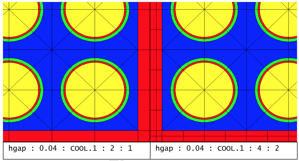
Fig. 3.2.1 Interassembly half gap meshing variants.

3.2.4.5. box - channel box geometry

box thick=Real [rad=*Real*] [hspan=*Real*] [Mbox=MNAME] [cothick=*Real*] [cobtm=*Real*] [cotop=*Real*]

[: t2 t3 … ti … tN
[: a2 a3 … ai … aN
[: b2 b3 … bi … bN
[: M2 M3 … Mi … MN
[: r2 r3 … ri … rN+1 ]]]]]

param	type	name	details	default
thick	Real	nominal thickness (cm)	must be > 0.0
rad	Real	inner corner radius (cm)	must be $\geq$ 0.0	0.0
hspan	Real	half inner span (cm)	——-See comments— —-
Mbox	MNAME	box material		_*
cothick	Real	interior cutout region thickness (cm)	thick > cothick $\geq$ 0.0	0.0
cobtm	Real	distance from box centerline to bottom of interior cutout region (cm)	hspan-rad > cobtm $\geq$ 0.0	0.0
cotop	Real	distance from box centerline to top of interior cutout region (cm)	cobtm $\geq$ cotop $\geq$ 0.0	cobtm

options for additional box zones
t_i	Real	zone thickness (cm)	must be $\geq$ 0
a_i	Real	distance from box centerline to bottom of zone cutout region (cm)	—–See comments— –
b_i	Real	distance from box centerline to top of zone cutout region (cm)	—–See comments— –
M_i	MNAME	zone material	—–See comments— –
ri	Real	zone inner corner radius (cm)	—–See comments— –

*By default, box material will be set to CAN.1 by “system BWR.” Otherwise box material is required.

Examples:

% simple
box 0.2

% rounded corner, rad 0.9
box 0.2 0.9

% rounded corner and user-defined inner span
box 0.2 0.9 6.7

% two zones
box 0.2 0.9 6.7
  : 0.2
  : 4.0
  : 4.3

Comments:

The box specifies the channel box geometry that surrounds the pinmap. The three primary dimensions of the channel box are the thickness (thick), the inner corner radius (rad), and the half inner span (hspan). Several additional dimensions for both box and cross are defined with respect to the channel box center. The channel box center is not to be confused with the lattice center: the former is the centroid of the inner channel box square boundary and the latter will depend on the wide and narrow gap dimensions provided on the hgap card. By default, the half inner span is equal to the half pin pitch multiplied by the number of pins on each side of the assembly (see npins and ppitch on the geometry<ASSM> card). If a cross card is applied, the default half inner span is increased by the half width of the interior cross buffer region (see hwidth on the cross card).

Additional channel box zones can be specified on the box card. The additional zones are useful for defining thick corner regions of the channel box. Each additional zone must have a user-defined thickness (t_i, i = 2 to N). Note that the starting index begins at “2” rather than “1” because the zone 1 thickness has already been defined by the “thick” input field.

“Cutout regions” may be defined in which a portion of the channel box zone is replaced by the corresponding hgap material along the horizontal and vertical centerlines of the channel box. The cutout region is defined by the distance from the channel box centerline to the bottom additional channel box zone (a_i) and the top of the channel box zone (b_i). The values of a_i and b_i determine the size of trapezoidal cutout region centered along each face of the channel box. The b_i value must be greater than or equal to the a_i value. The a_i value must be greater than or equal to the previous zone’s b_i value, i.e., b_i-1. By default, a₂ and b₂ are zero. If only M cutout regions are specified for N additional zones, i.e., M < N, both a_i and b_i is set to b_M for i = M+1 to N.

Additional zones can also have a different inner corner radius (r₂ … r_N). The outer corner radius of the last zone may also be specified (r_N+1). By default, r₂ is zero if rad is zero. If rad is greater than zero, the default value of r₂ is rad+thick. Similar rules apply for determining the default corner radii for additional zones if they are omitted in the input specification.

Additional zones can also have a different material (M_i). By default, M₂ is M_box. If additional materials are omitted in the input, the default value of M_i is M_i-1 for i = 3 to N.

The spatial mesh along each face of the channel box will be determined by the nf values specified on the hgap card.

The four examples listed above are displayed in Fig. 3.2.2. For additional examples, see the polaris.6.3 regression input files described at the beginning of Sect. 3.2.2.

See also:

geometry<ASSM>, hgap, cross

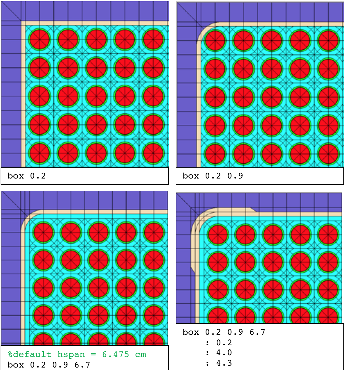
Fig. 3.2.2 Box card examples.

3.2.4.6. pin - pincell comprised of nested geometry zones of variable shape

pin PINID [size=*Real*]

: r1 r2 … ri … rN
: M1 M2 … Mi … MN [Mout]
[: S1 S2 … Si … SN]

param	type	name	details	default
PINID	Word\|Int	pin identifier
size	Real	pin size multiplicat ion factor	must be $\geq$ 1.0	1.0
r_i	Real	zone interior radius (cm)	r₁ must be > 0. Additional zones must be > r_i-1
M_i	MNAME	zone material	.1 added if given MCLASS, e.g., FUELFUEL.1
M_out	MNAME	outermost zone material	.1 added if given MCLASS	*
S_i		CIR or SQR or SQR(X)	circular zone or square zone with optional corner radius, X $\geq$ 0.0	CIR X=0.0

*If not specified, the material class MCLASS is taken from the channel card (M_chan) and set to the first member of that class, “M_chan.1.” For example if M_chan=”COOL,” then M_out= “COOL.1.”

Examples:

%standard fuel pin
pin 1 : 0.4096 0.418 0.475 : FUEL.1 GAP.1 CLAD.1

%2x2 water rod
pin W 2.0 : 1.6   1.7 : MOD.1 TUBE.1

%3x3 square water box (ATRIUM)
pin W 3.0 : 1.68 1.75 : MOD.1 TUBE.1 : SQR SQR

%noninteger size water rod (GE9x9)
pin W 1.76 : 1.16 1.259 : MOD.1 TUBE.1 COOL.2

Comments:

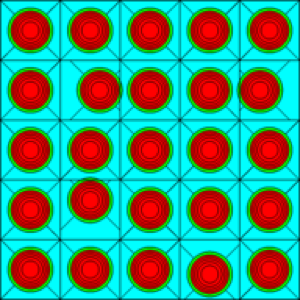
The pin card is one of the basic building blocks of the assembly model. pin and slab are the only geometry components which allows an integer (Int) identifier as well as a Word-all other geometric identifiers use Word. Note that the materials are required, except for the last M_out, which can be used to overwrite the material given by a channel for the outermost region in the pincell. The pin geometry is constructed from the inside out, using either circle zones (defined by the radius) or square zones (defined by the half-width, and optional corner radius). Different examples of pin geometries are displayed in Fig. 3.2.3. All meshing options for the pin are provided through the mesh card.

If the pin size is an integer value, the pin consumes a size $\times$ size subarray in the pinmap (e.g. 1 $\times$ 1, 2 $\times$times` 3, etc). If the pin size is noninteger, the pin consumes a ceil(size) $\times$ ceil(size) subarray in the pinmap. ceil(x) represents the ceiling function to round the value of x to the nearest integer greater than or equal to x. For size equal to 1.3, each instance of the pin will consume a 2 $\times$ 2 subarray in the pinmap. Each instance of a noninteger-sized pin must share a location with another instance of a noninteger-sized pin, but not necessarily the same pin. The shared location must be set to “_” in the pinmap. The identification of the shared location is necessary to determine the center of each pin. The pin center is at a distance of size*half pitch*sqrt(2) from the opposite corner of the shared location, along the diagonal of the pin boundary. An example of an integer-sized pins is displayed in Fig. 3.2.3. An example of noninteger-sized pins is displayed in Fig. 3.2.4.

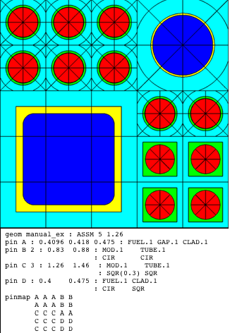
Fig. 3.2.3 Pin examples with different shape geometries

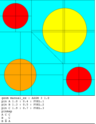
Fig. 3.2.4 Pin examples with noninteger pin size.

For additional examples, see the polaris.6.3 regression input files described at the beginning of Sect. 3.2.2

See also:

slab, pinmap, channel, mesh

3.2.4.7. pinmap - pin layout

pinmap PINID₁

PINID₂ …

PINID_i … PINID_N

param

type

name

details

default

PINID_i

Word|Int

list of

pin identifiers

supports full, quarter, or octant symmetry

quarter: assumes southeast (SE)

octant: assumes south-by-so utheast (SSE)

Examples:

%Westinghouse 17x17 pinmap in octant symmetry
pinmap
  2
  1 1
  1 1 1
  3 1 1 3
  1 1 1 1 1
  1 1 1 1 1 3
  3 1 1 3 1 1 1
  1 1 1 1 1 1 1 1
  1 1 1 1 1 1 1 1 1

%Westinghouse 17x17 pinmap in quarter symmetry
pinmap
  2 1 1 3 1 1 3 1 1
  1 1 1 1 1 1 1 1 1
  1 1 1 1 1 1 1 1 1
  3 1 1 3 1 1 3 1 1
  1 1 1 1 1 1 1 1 1
  1 1 1 1 1 3 1 1 1
  3 1 1 3 1 1 1 1 1
  1 1 1 1 1 1 1 1 1
  1 1 1 1 1 1 1 1 1

%Westinghouse 17x17 pinmap in full
pinmap
  1 1 1 1 1 1 1 1 1 1 1 1 1 1 1 1 1
  1 1 1 1 1 1 1 1 1 1 1 1 1 1 1 1 1
  1 1 1 1 1 3 1 1 3 1 1 3 1 1 1 1 1
  1 1 1 3 1 1 1 1 1 1 1 1 1 3 1 1 1
  1 1 1 1 1 1 1 1 1 1 1 1 1 1 1 1 1
  1 1 3 1 1 3 1 1 3 1 1 3 1 1 3 1 1
  1 1 1 1 1 1 1 1 1 1 1 1 1 1 1 1 1
  1 1 1 1 1 1 1 1 1 1 1 1 1 1 1 1 1
  1 1 3 1 1 3 1 1 2 1 1 3 1 1 3 1 1
  1 1 1 1 1 1 1 1 1 1 1 1 1 1 1 1 1
  1 1 1 1 1 1 1 1 1 1 1 1 1 1 1 1 1
  1 1 3 1 1 3 1 1 3 1 1 3 1 1 3 1 1
  1 1 1 1 1 1 1 1 1 1 1 1 1 1 1 1 1
  1 1 1 3 1 1 1 1 1 1 1 1 1 3 1 1 1
  1 1 1 1 1 3 1 1 3 1 1 3 1 1 1 1 1
  1 1 1 1 1 1 1 1 1 1 1 1 1 1 1 1 1
  1 1 1 1 1 1 1 1 1 1 1 1 1 1 1 1 1

%large central 2x2 water rod in 6x6 assembly
%pinmap must show adjacent Ws
pin W size=2 : 0.8
             : COOL
pinmap
F F F F F F
F F F F F F
F F W W F F
F F W W F F
F F F F F F
F F F F F F

Comments:

The pinmap card defines the layout of pin cells in the assembly. The symmetry is determined by the number of pin identifiers given on the card and must not be more general than the symmetry option given on the assembly geometry card (i.e., do not define a full pin map for a sym=SE assembly model). If the pin has a large size specifier, size>1, then the pinmap must reflect that with those pins occurring in blocks of size $\times$ size.

See also:

pin, control, insert

3.2.4.8. control<RODLET> - RCCA-type layout

control INAME: RODLET

PINID1
PINID2 …
PINIDi … PINIDN

param	type	name	details	default
INAME	Word	insert name
ETYPE	RODLET
PINID_i	Word\|Int	list of pin identifiers	same format as pinmap “_” indicate empty locations

Examples:

% B4C control rods
mat GAS.1  : FILLGAS
mat CLAD.1 : ZIRC4
mat MOD.1  : LW
mat TUBE.1 : SS304
mat CNTL.1 : B4C

pin B : 0.214  0.231 0.241 0.427 0.437 0.484 0.561 0.602
      : GAS    TUBE  GAS   CNTL  GAS   TUBE  MOD   CLAD

control  BankD  : RODLET
  _
  _ _
  _ _ _
  B _ _ B
  _ _ _ _ _
  _ _ _ _ _ B
  B _ _ B _ _ _
  _ _ _ _ _ _ _ _
  _ _ _ _ _ _ _ _ _

Comments:

Note that control elements and inserts share the INAME identifiers, so an insert and a control element cannot have the same name. Different control rod banks may be included in a single input file using more than one control card with unique INAMEs. The main difference between the inserts defined by control element and insert cards is that by default, control element materials are not depleted, whereas insert materials are depleted.

The outer dimensions of the tube must be included in the pin card that is inserted.

See also:

pinmap, control, insert, state

3.2.4.9. control<BLADE> - BWR control blade

control INAME : BLADE hwgthck=Real sththck=Real cslnth=Real
[sthmat=*MNAME*] [csmat=*MNAME*] [hcsthck=*Real*] [wgcrv=*Real*]
: ID1 ID2 … IDN
: L1 L2 … LN
[: N1 N2 … NN]

param	type	name	details	default
hwgthck	Real	half blade wing thickness (cm)	must be >0
sththck	Real	sheath thickness (cm)	must be >=0
cslnth	Real	central support length (cm)	must be >=hwgthck
sthmat	MNAME	sheath material		STRUCT.1^*
csmat	MNAME	central support material		STRUCT.1^*
hcsthck	Real	half central support thickness (cm)	must be >0	hwgthck
wgcrv	Real	wing tip radius (cm)	must be >=0	0
ID_i `	Word\|Int	pin or slab identifier	——- See comments ———-
L_i	Real	length of section i	——- See comments ———-
N_i	Real	# of pins or slabs in section i	——- See comments ———-
*Default values for shtmat and csmat are set by “system BWR.” If “system BWR” is omitted, the material definitions are required.

Comments:

The blade card defines a control blade geometry. The control blade identifier (INAME) can be used to insert the control blade using state or add statements to define histories or branches respectively. INAME=yes inserts the control blade into the northwest corner of the lattice.

The control blade geometry is described with reference to the blade wing on the northern edge of the lattice in Fig. 3.2.5. The blade wing on the west edge is a reflection of the northern edge wing along the diagonal symmetry line that extends from the northwest corner to the southeast corner of the lattice.

The two primary regions of the blade are the central support and the active blade wing. The central support has a length (cslnth), half width (hcsthck), and material (csmat). The central support half width is the vertical distance between the north face of the lattice and the south boundary of the central support. The central support length is the horizontal distance from west face of the lattice to the east boundary of the central support. See Fig. 3.2.5 for details.

The active portion of the blade wing begins at the east boundary of the central support. The active portion has a half width (hwgthck), sheath thickness (sththck), sheath material (sthmat), and wing tip radius (wgcrv). The half width is the vertical distance between the north face of the lattice and the southern boundary of the active blade wing, including the sheath. The wing tip radius can be any nonnegative number. If the radius is zero, the wing tip is a straight edge.

The active portion of the blade wing is subdivided into sections. Each section has a length (L_i), and identifier associated with a pin or slab (ID_i), and the number of pins or slabs for each section (N_i). The list of section lengths and section identifiers is required and must have consistent list lengths. The final list for number of pin/slabs per section is optional. If omitted, the default number of pin or slabs per section is one.

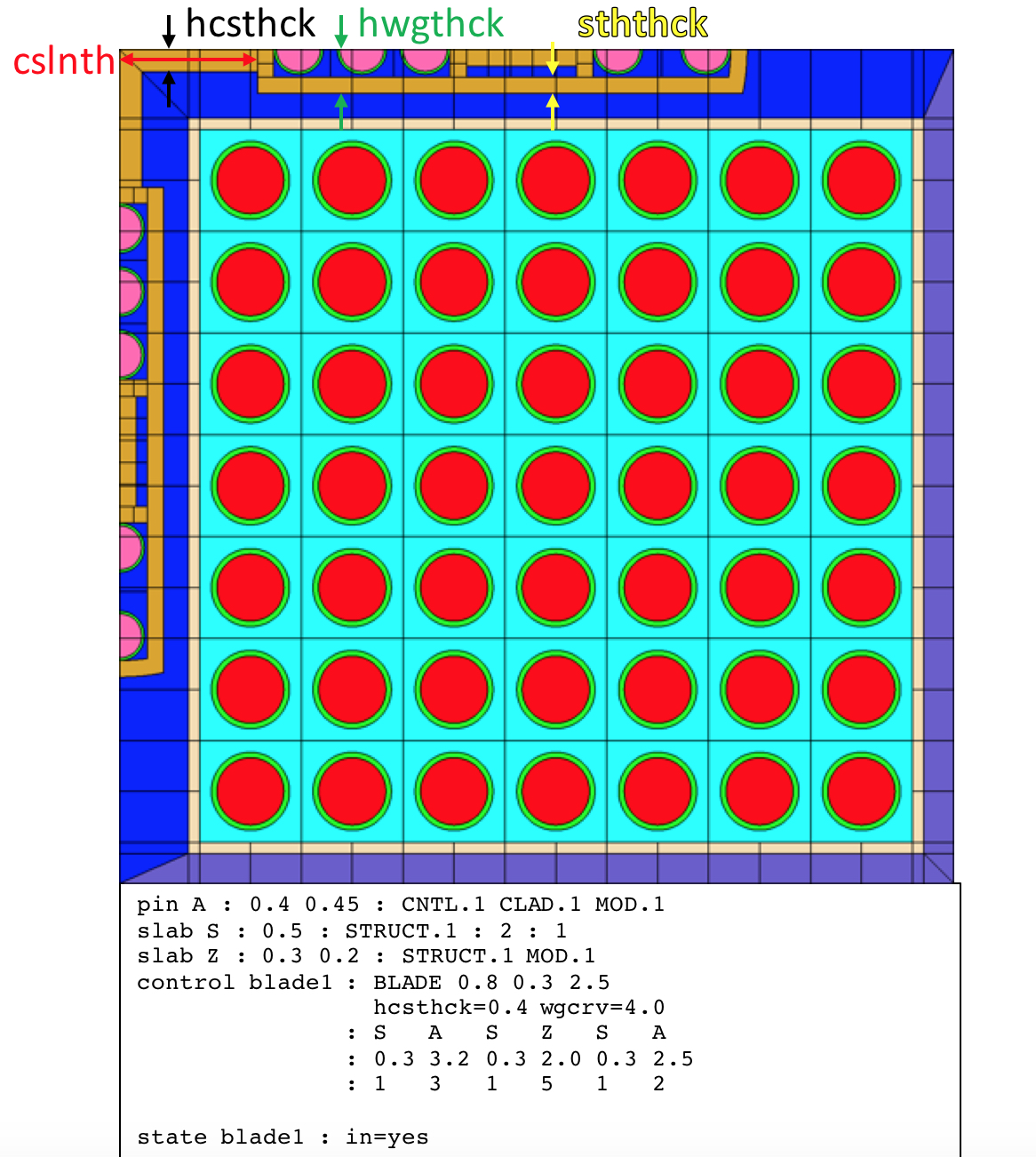
Fig. 3.2.5 Control blade example.

If there is only one pin in a pin section, the pin is placed in the section center. If there are multiple pins, the first and last pin are positioned flush against the west and east section boundary respectively, and the interior pins are uniformly spaced between the two edge pins. Slab sections are built from the blade centerline in the vertical direction towards the interior sheath boundary. Each slab zone has width equal to the section length. Each slab zone can be subdivided in the vertical direction by the zone nx parameter on the slab card. The slab zone can be subdivided in the horizontal direction by the product of the zone ny parameter and the number of slabs in the blade wing section.

The blade is further subdivided by the mesh nf/nd settings for hgap material in the north and west bypass region, typically MOD.1 for models that include system BWR.

3.2.4.10. insert - insert layout

insert INAME:

PINID1
PINID2 …
PINIDi … PINIDN

param

type

name

details

default

INAME

Word

insert name

PINID_i

Word|Int

list of

pin identifiers

same format as pinmap

“_” indicate empty locations

Examples:

%pyrex inserts
pin P : 0.214  0.231 0.241 0.427 0.437 0.484 0.561 0.602
      : GAS    TUBE  GAS   BP.3  GAS   TUBE  COOL  CLAD

insert PyrexInserts :
  _
  _ _
  _ _ _
  P _ _ P
  _ _ _ _ _
  _ _ _ _ _ P
  P _ _ P _ _ _
  _ _ _ _ _ _ _ _
  _ _ _ _ _ _ _ _ _

Comments:

The insert card defines a set of pins to be used to model inserts such as WABA. When the insert is “in,” the insert pins replace overlapping regions of the pins defined on the assembly pinmap. An underscore (_) is used to indicate locations without inserts. See the notes on the control<RODLET> card for additional guidelines.

See also:

pinmap, control, insert

3.2.4.11. slab - slab geometry

slab [SLABID]

: t1 t2 … ti … tN
: M1 M2 … Mi … MN
[: nx1 nx2 … nxi … nxN ]
[: ny1 ny2 … nyi … nyN ]

param	type	name	details	default
SLABID	Word	slab geometry identifier		reflector GNAME
t_i	Real	list of slab thicknesses	units: cm
M_i	MNAME	list of material names
meshing options
nx_i	Int	list of number of x-divisions		1
ny_i	Int	list of number of y-divisions		1

Examples:

% a reflector definition
% 2.22 cm of baffle
% 15 cm of moderator
geom ReflectorNode : REFL 17.22
  slab 2.22 15 : BAFFLE.1  MOD.1

Comments:

The slab card may be used to define three things: (1) the materials and thicknesses of a reflector initiated on a geometry card, (2) slabs in a control blade, and (3) spacer grids. If the first argument identifier is not present, then the first purpose of describing the various material thicknesses in a reflector is assumed. The meshing options allow each material slab to be spatially refined in x and y, increasing the number of cells in the transport problem. The meshing option for the number of x divisions creates the equivalent of additional “sub-slabs” in each user-defined slab thickness. The y-divisions create additional cells vertically. The default of one y-division corresponds to the entire assembly.

See also:

geometry<REFL>

3.2.4.12. cross - cross geometry

cross hwidth=Real lthick=Real
[Mcross=MNAME] [row=Int] [Min=MNAME] [ld=Int] [Mout=MNAME]
[ : x1 x2 … xN]
[ : y1 y2 … yN]
[ : yin1 yin2 … yinN]
[ : nx1 nx2 … nxN-1]
[ : ny1 ny2 … nyN-1]

Comments:

The cross card performs two tasks. First, it subdivides the pinmap into four subarrays, optionally adding a horizontal and vertical gap between the subarrays. The row parameter is uses to subdivide the pinmap. If the pinmap is 10 $\times$ 10 and row=5, each of the four subarrays is 5 $\times$ 5. If the pinmap is 10 $\times$ 10 and row=4, the northwest subarray is 4 $\times$times`6, the southwest subarray is 6 $\times$ 4, and the southeast subarray is 6 $\times$ 6. The hwidth parameter controls the half-spacing of the horizontal and vertical gap in between the subarrays. The hwidth parameter must be $\geq$ 0.0 and if hwidth is > 0.0, the gap is filled with material M_out (default is COOL.2 with system BWR).

The second task is the insertion of the cross structure into the lattice geometry. The process is described with reference to the example in Fig. Fig. 3.2.6. In the example, the pinmap is 9 $\times$ 9 and row=3, hwidth=1.5, and hspan=10.5. The top left plot contains the four following lines:

the line in the center of the vertical cross gap,
the line in the center of the horizontal cross gap,
the diagonal line from the northwest (NW) channel box corner to the southeast (SE) corner, and
the diagonal line, perpendicular to line 3, passing through the intersection of line 1 and line 2.

These four lines intersect and form 8 separate regions, i.e., octants, within the channel box interior. The intersection point, i.e., cross center, is not necessarily equal to the box center as shown in this example. In the top left plot, the red triangle represents the WNW octant. In the bottom left plot, the red triangle represents the SSE octant.

% Centered cruciform flow channel
cross   0.625  0.08  5
: -6.86 -6.53 -5.20 -4.81 -3.77 -3.39 -2.05  0.0  2.05  3.39  3.77  4.81  5.20  6.53  6.86
: 0.625  0.0   0.0   0.24  0.24  0.0   0.0  2.05  0.0   0.0   0.24  0.24  0.0   0.0   0.625

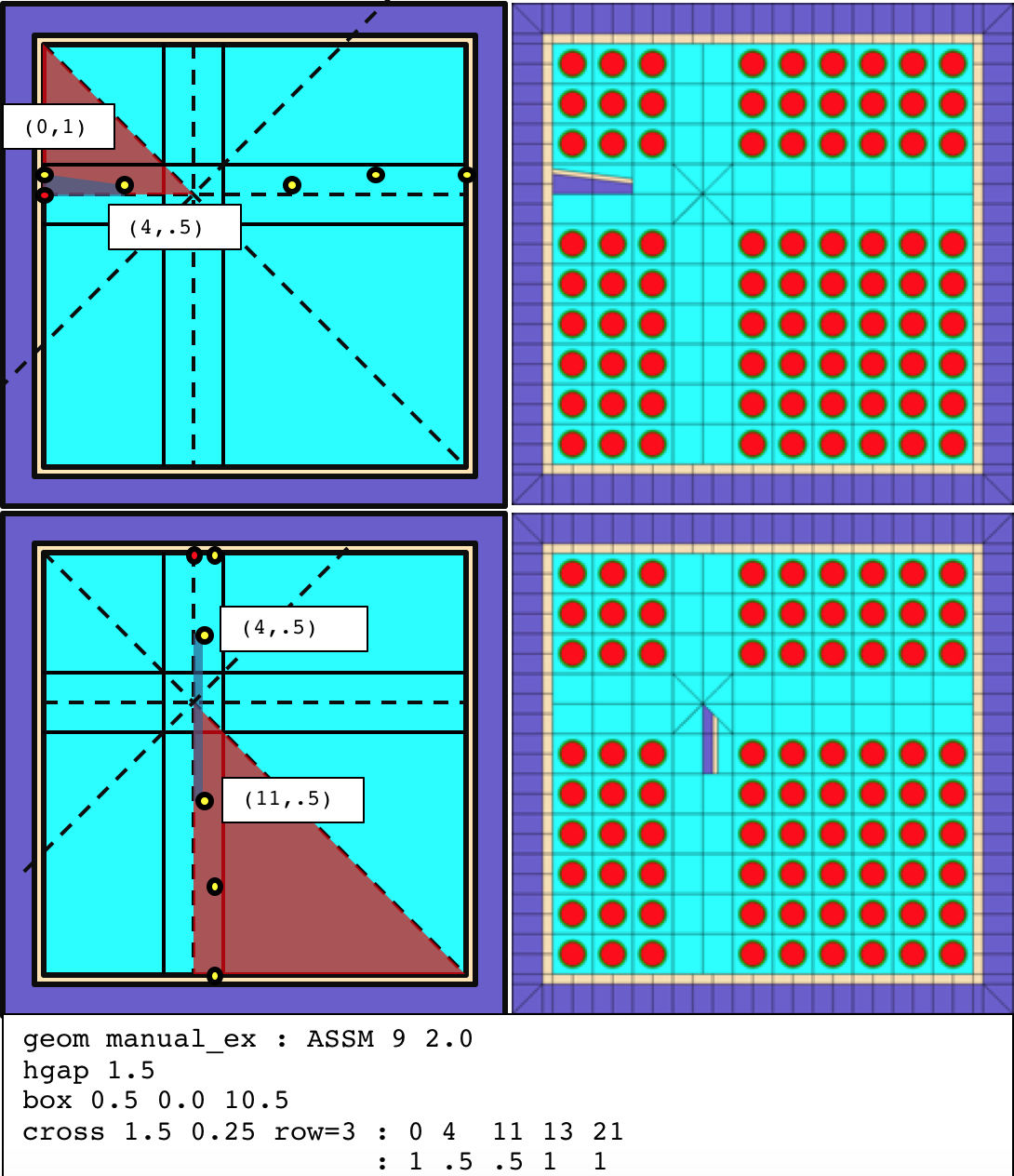
Fig. 3.2.6 Construction of the BWR cross geometry (full example shown later).

The cross structure is defined be a series of vertices (x_i, y_i). Shown as yellow points in the top left plot, the cross vertices are defined based on an origin displayed as the red point, which is the intersection of the inner west edge of the channel box and the horizontal line in that passes through the cross center.

The top plots demonstrate how Polaris inserts a section of the cross into the WNW octant. In the top left plot, the blue polygon is constructed based on the first two vertices defined on the cross card: (0.0,1.0) and (4.0,0.5). The intersection of the blue polygon and red polygon is inserted into the lattice and filled with cross interior material (M_in). The liner is then inserted above the blue polygon, padded by the liner thickness (lthick), and clipped by WNW red polygon if needed.

Similarly, the bottom plots demonstrate insertion into the SSE octant. For SSE insertions, the origin and the cross vertices are rotated 90 degrees about the cross center. The blue polygon is constructed from the second and third vertices on the cross card: (4.0,0.5) and (11,0.5). The intersection of the blue polygon and red polygon is inserted into the lattice and filled with cross interior material (M_in). The liner is then inserted above the blue polygon, padded by the liner thickness (lthick), and clipped by SSE red polygon if needed.

For each consecutive set of cross vertices, Polaris inserts a polygonal region into each of the 8 octants. The cross vertices are entered in the input as an x-values list followed by a y-values list of the same length. The coordinate system of the x- and y- lists is displayed in the top left plot of Fig. 3.2.6. The coordinate system is transformed based on the following rules for each octant:

WNW, ENE: no transform,
NNW, SSW: reflected across the diagonal line from NW to SE channel box corners,
NNE, SSE: rotated 90 degrees about the cross center, and
ESE, WSW: reflected across the line in the center of the horizontal cross gap.

The cross liner is inserted above the cross vertex values. The liner has a uniform thickness (lthick) and uniform material (M_cross). The uniform liner thickness is constructed with a miter joint at each cross vertex as shown in the following diagram:

After the set of y-values on the cross card, an optional list of interior y-values can be specified. The length of the interior y-values list must be equal to the length of the x- and y- lists. The optional interior y-values list is used to split the polygons into two material regions as shown in the following diagram:

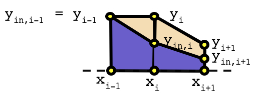
For the left-hand polygon, y_in,i-1 is the same as y_i-1, but y_in,i is less than y_i. In this scenario, the trapezoid region is filled with M_in, and the triangular region is filled with M_cross. Similarly for the right-hand polygon, the lower trapezoid is filled with M_in and the upper trapezoid is filled with M_cross. Note that the uniform liner above the y-values is not shown for simplicity.

The interior y-list values can be specified in one of two ways. First, a positive value may be entered that is greater than or equal to zero and less than or equal to the corresponding y-value. Second, a negative value may be entered that represents the relative distance of the interior y-value below the corresponding y-value. Note the Polaris input processor interprets “-0” different than “0”. “-0” implies that the internal y-value is the same as the y-value. “0” implies that the internal y-value is zero. If the interior y-list is omitted, the default for all internal y-values is “-0”, i.e., the polygon regions defined are completely filled with M_in.

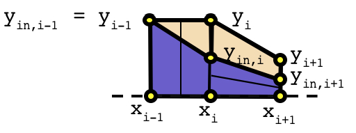
In addition to the interior y-values list, two additional lists can be used to refine the spatial mesh in the x- and y- directions. The list of nx- and ny- values subdivide the polygon regions along the x- and y- directions respectively. Both lists must have one less entry than the x-, y-, and y_in- lists. If omitted, the default values for both the nx- and ny- lists are 1, i.e., no additional spatial refinement is applied to the polygon regions. For refinement in the y-direction, only the M_in material is refined. The following diagram shows nx=2 refinement for the left polygon and ny=2 refinement for the right polygon:

The full cross example from Fig. 3.2.6 is displayed in the top left plot of Fig. 3.2.7. The bottom plot shows a centered cross structure with a diamond water box and empty pins surrounding the water box.

For additional examples, see the polaris.6.3 regression input files described at the beginning of Sect. 3.2.2.

See also:

box, system BWR, pinmap

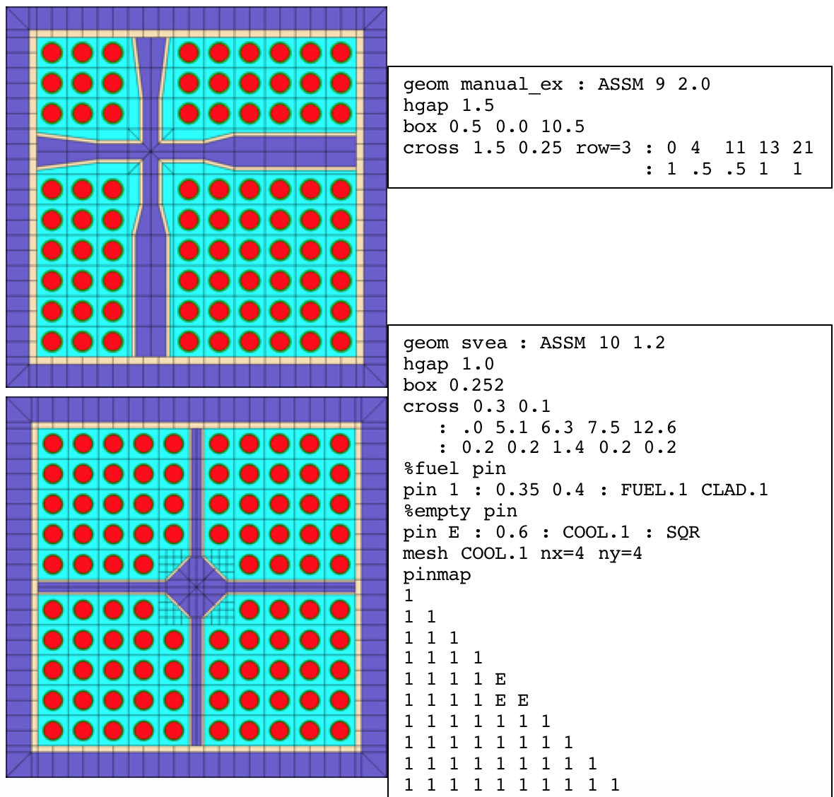
Fig. 3.2.7 Additional cross examples.

3.2.4.13. dxmap and dymap - pin-by-pin displacement maps

dxmap d₁ d₂ … d_i … d_N

dymap d₁ d₂ … d_i … d_N

param	type	details	default
d_i	Real	pin center displacement value in the x or y direction (cm)	0.0

Comments:

The dxmap and dymap cards displace pins from their natural position in the geometry (see comments for the pin card). If displacement maps are required, both the dxmap and dymap must be specified in the input and they must have the same length. However, the length of the displacement maps does not have to equal of length of the pinmap if the displacement maps have reduced symmetry. For integer-sized pins greater than 1, the displacement value should be entered in the northwest corner element of the size $\times$ size subarray. For noninteger-sized pins, the displacement value should be in the corner element opposite of shared corner location. Note the following symmetry restrictions for the displacement maps:

dy_i value must be zero on a horizontal symmetry line for an odd $\times$ odd pinmap,
dx_i value must be zero on a vertical symmetry line for an odd $\times$ odd pinmap, and
dx_i must equal dy_i for an element on a diagonal symmetry line.

Examples:

dxmap
0  0.0  0.0  0.0  0.0
0  0.2  0.0  0.0 -0.2
0  0.0  0.0  0.0  0.0
0  0.0  0.0  0.0  0.0
0  0.0  0.0  0.0  0.0
dymap
0  0.0  0.0  0.0  0.0
0  0.0  0.0  0.0  0.0
0  0.0  0.0  0.0  0.0
0  0.2  0.0  0.0  0.0
0  0.0  0.0 -0.1  0.0

See also:

pinmap

3.2.4.14. mesh - advanced material dependent meshing options

mesh MSPEC : [m=Real] [nx=Int] [ny=Int] [mx=Real] [my=Real]

[nr=Int] [ns=Int] [mr=Real] [ms=Real]

[nf=Int] [nd=Int] [mf=Real] [md=Real]

param	type	name	details	default
MSPEC	MCLASS \|MNAME	material identifier
nx	Int	# of x divisions	must be >0	MeshNumX^*
ny	Int	# of y divisions	must be >0	MeshNumY^*
nr	Int	# of radial rings	must be >0	MeshNumRings^*
ns	Int	# of radial sectors	must be nonzero	MeshNumSectors^*
nf	Int	# of faces/pin	must be >0	2^**
nd	Int	# of gap divisions	must be >0	1
meshing multipliers
m	Real	global multiplier	must be >0	1.0
mx	Real	x divisions	must be >0	1.0
my	Real	y divisions	must be >0	1.0
mr	Real	radial rings	must be >0	1.0
ms	Real	radial sectors	must be >0	1.0
mf	Real	faces/pin	must be >0	1.0
md	Real	gap divisions	must be >0	1.0

^* The global mesh default values are set on the option <GEOM> card using the parameter name in the table above.

^** Default number of faces per pin is 1. Default is 2 for system BWR or system PWR.

Examples:

mesh COOL : nr=3 ns=4 nx=2 ny=2 %coolant mesh: 3 ring, 4 sectors, 2 in x and y

mesh MOD.1 : nf=2 nd=4          %mesh used for wide gap (MOD.1): nf=2 nd=4

mesh MOD.2 : nf=2 nd=3          %mesh used for narrow gap (MOD.2): nf=2 nd=3

mesh FUEL : mr=2.0              %double the fuel radial mesh

mesh FUEL.2 : m=3.0             %triple all mesh values for FUEL.2

mesh CLAD : ms=0.5              %coarsen the clad sector mesh by a factor of 1/2.

Comments:

Polaris supports three different mesh types: 1) cylindrical mesh for CIR shapes in the pin card, 2) Cartesian mesh for SQR shapes in the pin card, and 3) a special Cartesian mesh for the region external to the pinmap region. As shown in the examples above, the mesh card is used to define, refine, or coarsen the mesh parameters for one or more of the mesh types associated with a given material class or material name. The default values for mesh parameters are defined through the option<GEOM> card and the system card. The default values on the option<GEOM> card are nr=1, ns=1, nx=1, ny=1, nf=1, nd=1, and MeshMult=1.0. The “MeshMult” multiplier from the option<GEOM> is a global mesh multiplier applied in conjunction with any material-specific multiplier (see option<GEOM> example for details). If system BWR or system PWR is applied, new default values include nf=2, ns=8, and nr=2 (only for the channel material class). If the final mesh value is noninteger, Polaris rounds down to determine the applied value.

3.2.4.15. detector - insert a detector geometry

det DNAME : PINID at=PINID|GNAME loc=String

: rx=RSPEC fmat=MNAME rmat=MNAME

Examples:

% declare detector materials
mat DET.2 : SS304 %transmitter
mat DET.3 : Al 2.7 %active material matrix (with u235 dopant not modeled)

% declare detector geometry
% - transmitting wire
% - active material
% - sheath
pin PD : 0.03 0.04 0.0787
: DET.2 DET.3 TUBE.1

%u235 for reaction rate material
mat DET.1 : detu 1e-5
   comp detu : WT u235=99.9 u238=0.1

% place detector D1, described by pin PD
% into instrument tube pin.IT, at the center
% with signal proportional to fission in material DET.1
% but with flux inside material matrix DET.3
det D1 : pin.PD at=pin.IT loc=CENTER
: R(n,FIS) fmat=DET.3 rmat=DET.1

% enable detector output in XFile16
opt FG DetectorEdit=D1

Comments:

The detector card is not intended to produce arbitrary reaction rates, but model a simple, discrete detector inserted into the geometry. The first line of detector input defines the detector and where it should be placed. The second line of input defines the “signal” the detector produces. The most complex piece of the input is the reaction specificer (RSPEC) which denotes the units (reaction rate or energy rate), incident particle, and type of reaction. For example, neutron absorption rate would be denoted “R(n,ABS)” and gamma energy deposition rate “E(g,CAP)”.

The detector signal is collected for the material specified as the flux material, “fmat”. In some cases, e.g. PWR fission detector modeling, it is desirable to model a reaction rate for fissile material that does not exist, e.g. a U-235 fission rate in an gaseous fission chamber that does not have trace amounts of U-235 present in the composition definition. The optional reaction material, “rmat”, gives a way to specify this type of scenario. In this case the “fmat” would be a physical material in the model like the detector fill gas whereas the “rmat” would be another material (not present in the model) with composition and temperature defined appropriately.

3.2.5. Materials

A material contains two main types of information: (1) the composition, or distribution of nuclides, and (2) the properties which include basic (required) properties like density and temperature, and as well as (optional) properties like soluble poison content, void, or grid spacer smearing. The composition is defined by a composition card. The basic specification for a material is shown below.

[mat MNAME : CNAME [dens=*Real*] [temp=*Real*] [: properties]]

argument	type	name	details	default
MNAME= MCLASS.MSUB	Word. Int	material name	used to reference this material
CNAME	Word	composition name
dens	Real	density	basic property units: g/cm³	composition reference density, if defined
temp	Real	temperature	basic property units: K	293
properties	Word=Value	properties	extra properties are defined with property cards	no extra properties

A material name has two parts, the material class, or MCLASS, and a member identifier, or MSUB. For example, FUEL.2 has an MCLASS=FUEL and an MSUB=2. All properties are defined by MCLASS. The composition referenced by CNAME is created with a composition card, as shown below.

[comp CNAME : CTYPE arguments]

Table 3.2.4 :class: longtable
argument	type	name	details	default
CNAME	Word	composition name	used to reference this composition later in materials and property definitions
CTYPE	-	composition type
	General Composition Constructors
	NUM	number fraction
	WT	weight fraction
	FORM	Formula
	CONC	Concentrations
	Reactor Composition Constructors
	LW	borated light water
	UOX	uranium oxide fuel
arguments	-	remaining arguments	depends on CTYPE

Additional properties are defined with the property card, which defines the property PNAME for a material class MCLASS. The property type, PTYPE, determines the remaining arguments.

prop PNAME MCLASS : PTYPE arguments

argument	type	name	details	default
PNAME	Word	property name	used to reference this property
PTYPE	PTYPE	property type
	SOLP	soluble poison	used to define soluble boron content
arguments	-	remaining arguments	depends on PTYPE

3.2.5.1. material - material initialization

mat MNAME : CNAME [dens=Real] [temp=Real]

[: p₁=val₁ p₂=val₂ … p_i=val_i … p_N=val_N]

argument	type	name	details	default
MNAME	Word. Int	material name	uses form MCLASS.MSUB
CNAME	Word	composition name
dens	Real	density	basic property units: g/cm³	composition reference density
temp	Real	temperature	basic property units: K	293
p_i =val_i	PNAME=Value	properties	additional properties	0

Examples:

% define a gas gap material
mat GAP.1  : FILLGAS

% define a 3.5% enriched fuel material
comp uox_e350 : UOX 3.5
mat FUEL.1 : uox_e350 dens=10.257 temp=900

% define a cladding material
mat CLAD.1 : ZIRC4

% define a guide tube material
mat TUBE.1 : SS304

% define a control rod material
mat CNTL.1 : AIC

Comments:

Material properties may be set on either a material card or on a state card. If a temperature is specified rather than a density, the “temp=” key must be used to skip over the density argument.

See also:

state, composition, property

3.2.5.2. composition<NUM|WT> – general atom/wt fraction

comp CNAME: NUM|WT
[scale=<PCT>|ABS|PPM]
[norm=Bool]
[refdens=Real]
[structure=Function]
id1=val1 id2=val2 … idi=vali … idN=valN

Examples:

% create a plutonium vector and then plutonium oxide
comp puvec : WT scale=PCT
  Pu238=1.2
  Pu239=63.3
  Pu240=21.0
  Pu241=8.6
  Pu242=5.9
comp puox : FORM puvec=1 O=2

% create an 85/10/5 Ag/In/Cd composition
% using 10% In, 5% Cd,
% and filling the remainder up to 100% with Ag
comp aic : WT In=10 Cd=5 Ag=-100

Comments:

IDs in weight or number fraction-based compositions may be any of the following:

nuclide IDs (Int), e.g., 92235,
nuclide names (Word), e.g., U235 or u235,
element Z numbers (Int), e.g., 92,
element names (Word), e.g., U or u, or
other composition names (CNAME).

See also:

composition<FORM>

3.2.5.3. composition<FORM> - general chemical formula

comp CNAME : FORM

[refdens=Real]
[structure=Function]
id1=val1 id2=val2 … idi=vali … idN=valN

param	type	name	details	default
CNAME	Word	composition name
CTYPE	FORM	formula
refdens	Real	reference density	default density for materials using this composition units: g/cm³	*
structure	Function	structure	see Structure names	FREE
id_i =val_i	Word\|Int=Real	id/value pairs	see acceptable id forms below values in atoms per molecule (e.g., H₂O is given as “H”=2 “O”=1)

*The density property must be defined for each material either explicitly on the material card itself or implicitly through the “reference density” of the material’s composition.

Examples:

% define Gd2O3 using element names
% (using elements implies natural abundances used in isotopics)
comp gd2o3 : FORM Gd=2 O=3

% define Gd2O3 using 100% Gd 155
comp gd2o3 : FORM Gd155=2 O=3

% define D2O using nuclide IDs and element names
comp d2o : FORM 1002=2 8000=3
comp d2o : FORM H2=2 O=3

Comments:

IDs in formula-based composition may be any of the following:

nuclide IDs (Int), e.g., 92235,
nuclide names (Word), e.g., U235 or u235,
element Z numbers (Int), e.g., 92,
element names (Word), e.g., U or u, or
other composition names (CNAME).

See also:

composition<NUM|WT>, composition<CONC>

3.2.5.4. composition<CONC> - general number density

comp CNAME : CONC [refdens=Real]

id₁=val₁ id₂=val₂ … id_i=val_i … id_N=val_N

param	type	name	details	default
CNAME	Word	composition name
CTYPE	CONC	concentration
refdens	Real	reference density	default density for materials using this composition units: g/cm³	**
id_i =val_i	Int=Real	id/value pairs	see acceptable id forms below note: cannot use other CNAMEs for IDs in CONC input units: #/barn-cm

**A reference density is automatically calculated from concentrations input. If specified, it will simply scale up concentrations linearly.

% pyrex composition
comp pyrex_e125 : CONC
         5010=9.63266E-04
         5011=3.90172E-03
         8016=4.67761E-02
        14028=1.81980E-02
        14029=9.24474E-04
        14030=6.10133E-04

% fuel composition
comp uox_e310_gd180 : CONC
        92234=3.18096E-06
        92235=3.90500E-04
        92236=1.79300E-06
        92238=2.10299E-02
        64152=3.35960E-06
        64154=3.66190E-05
        64155=2.48606E-04
        64156=3.43849E-04
        64157=2.62884E-04
        64158=4.17255E-04
        64160=3.67198E-04
         8016=4.53705E-02

% wet annular burnable absorber (WABA) composition
comp waba : CONC
         5010=2.98553E-03
         5011=1.21192E-02
         6000=3.77001E-03
         8016=5.85563E-02
        13027=3.90223E-02

Comments:

IDs in concentration-based composition may be any of the following:

nuclide IDs (Int), e.g., 92235;
nuclide names (Word), e.g., U235 or u235;
element Z numbers (Int), e.g., 92;
element names (Word), e.g., U or u; and
SCALE-specific Nuclide IDs (Int), e.g., 3006000 (Only available for comp(CONC) card).

Other composition names (CNAME) cannot be used in a concentration definition. To easily ensure consistency of input when comparing codes, the composition input should be used in the concentrations described here. In all other cases, the other composition constructors are recommended because they are much simpler and easier to use.

See also:

composition<FORM>, composition<NUM|WT>

3.2.5.5. composition<LW> - borated light water

comp CNAME : LW [borppm=Real] [refdens=Real]

param	type	name	details	default
CNAME	Word	composition name
CTYPE	LW	light water
borppm	Real	boron	parts per million by weight of natural boron (B) in light water (H₂ O)	*
refdens	Real	reference density	default density for materials using this composition units: g/cm³	0.0

*The density property must be defined for each material either explicitly on the material card itself or implicitly through the “reference density” of the material’s composition.

Examples:

% define a 600ppm boron moderator composition
comp mod_600ppm : LW 600

% same composition using FORM and WT
comp mod : FORM H=2 O=1
comp mod_600ppm : WT scale=PPM norm=yes
                  mod=1e6 B=600

Comments:

Internally, the borated light water composition is built from composition<FORM> and composition<WT> cards assuming natural boron. To use different boron isotopics such as depleted or enriched boron, the more general composition cards should be used.

See also:

composition<FORM>, composition<WT>

3.2.5.6. composition<UOX> -UO₂ fuel

comp CNAME : UOX enr=Real [bu=Real] [refdens=Real]

param	type	name	details	default
CNAME	Word	composition name
CTYPE	UOX	uranium dioxide
enr	Real	enrichment	U-235 wt. % (see composition<ENRU> for formula)
bu	Real	burnup	only available for $0\leq bu \leq 100$ units: GWd/MTU	0*
refdens	Real	reference density	default density for materials using this composition units: g/cm³	**

*Note that the burnup parameter should not be specified. It is a future option to create a fixed, representative, burned fuel composition. The composition is interpolated using linear interpolation from an internal burnup- and enrichment-dependent data matrix.

**The density property must be defined for each material either explicitly on the material card itself or implicitly through the “reference density” of the material’s composition.

Examples:

% define a 4.95% enriched fuel composition with a reference density
comp uox_495 : UOX 4.95 refdens=10.25

% same result as above
comp u_495 : ENRU 4.95
comp uox_495 : FORM u_495=1 O=2

Comments:

Internally, the UO₂ composition is built from composition<FORM> and composition<ENRU> cards.

See also:

composition<ENRU>, composition<FORM>

composition<USI> – U₂Si₃ fuel

comp CNAME : USI enr=Real [bu=Real] [refdens=Real]

param	type	name	details	default
CNAME	Word	composition name
CTYPE	USI	uranium silicide
enr	Real	enrichment	U-235 wt. % (see composition<ENRU> for formula)
bu	Real	burnup	only available for $0\leq bu \leq 100$ units: GWd/MTU	0*
refdens	Real	reference density	default density for materials using this composition units: g/cm³	**

*Note that the burnup parameter should not be specified. It is a future option to create a fixed, representative, burned fuel composition. The composition is interpolated using linear interpolation from an internal burnup- and enrichment-dependent data matrix.

**The density property must be defined for each material either explicitly on the material card itself or implicitly through the “reference density” of the material’s composition.

Examples:

% define a 4.95% enriched fuel composition with a reference density
comp usi_495 : USI 4.95 refdens=11.54

% same result as above
comp u_495 : ENRU 4.95
comp usi_495 : FORM u_495=2 Si=3

Comments:

Internally, the U₂Si₃ composition is built from composition<FORM> and composition<ENRU> cards.

See also:

composition<ENRU>, composition<FORM>

3.2.5.7. composition<UN> - UN fuel

comp CNAME : UN enr=Real [n15enr=Real][bu=Real] [refdens=Real]

param	type	name	details	default
CNAME	Word	composition name
CTYPE	UN	uranium nitride
enr n15enr	Real Real	enrichment nitrogen enrichment	U-235 wt. % (see composition<ENRU> for formula) N-15 wt. %	100%*
bu	Real	burnup	only available for $0\leq bu \leq 100$ units: GWd/MTU	0**
refdens	Real	reference density	default density for materials using this composition units: g/cm³	***

* Natural nitrogen is 0.4 wt. % ¹⁵N, but the reactivity penalty of ¹⁴N warrants using the highest ¹⁵N composition possible.

**Note that the burnup parameter should not be specified. It is a future option to create a fixed, representative, burned fuel composition. The composition is interpolated using linear interpolation from an internal burnup- and enrichment-dependent data matrix.

***The density property must be defined for each material either explicitly on the material card itself or implicitly through the “reference density” of the material’s composition.

Examples:

% define a 4.95% enriched fuel composition with a reference density
comp usi_495 : UN 4.95 refdens=11.3

% same result as above
comp u_495  : ENRU 4.95
comp un_495 : FORM u_495=1 7015=1

% define a 3.25% enriched fuel composition with a reference density and
% specify natural 15N composition
Comp un_495 : UN 3.25 refdens=11.3 n15enr=0.4

Comments:

Internally, the uranium nitride composition is built from composition<FORM>, composition<WT>, and composition<ENRU> cards.

See also:

composition<ENRU>, composition<FORM>

3.2.5.8. composition<ENRU> – enriched uranium

comp CNAME : ENRU enr=Real [refdens=Real]

param	type	name	details	default
CNAME	Word	composition name
CTYPE	UOX	uranium dioxide
enr	Real	enrichment	*U-235 wt. %
refdens	Real	reference density	default density for materials using this composition units: g/cm³	**

*The following formula from [POLARISGod14] is used to determine the ²³⁴U and ²³⁶U wt% from the ²³⁵U enrichment. Note that this formula is only valid for U-235 enrichments less than 10 wt%.

w_u234 = 0.007731*(enr) ^1.0837

w_u236 = 0.0046*enr

w_u238 = 100 - w_u234 - enr - w_u236

**The density property must be defined for each material either explicitly on the material card itself or implicitly through the “reference density” of the material’s composition.

Examples:

% 5% enriched metal fuel
comp umetal : ENRU 5

Comments:

This composition for enriched uranium is used internally to create uranium oxide, silicide, and nitride fuels using the composition<UOX>, composition<USI>, and composition<UN> cards.

See also:

composition<UOX>, composition<USI>, composition<UN>

3.2.5.9. composition library (pre-defined)

The Polaris composition library contains predefined compositions that may be used without a constructor by simply referencing the CNAME below. Each predefined library composition has a reference density, so it can be used directly on a material card.

Table 3.2.5 Standard molecular compositions
CNAME	Description
H2O B4C Er2O3 Gd2O3 SiC ZrH Zr5H8 ZrH2 fillgas Cr2O3 Al2O3 BeO	light water with structure=BOND(H2O) Boron carbide burnable poison material Erbium oxide burnable poison material Gadolinium oxide burnable poison material Silicon carbide zirconium hydride alloy with structure=CRYS(orthorhombic_zrh) zirconium hydride alloy with structure=CRYS(cubic_zrh) zirconium hydride alloy with structure=CRYS(tetragonal_zrh) Helium gas Chromium dioxide (chromia, Cr₂O₃) Aluminum dioxide (alumina, Al₂O₃) Beryllium dioxide (beryllia, BeO)

Table 3.2.6 Standard reactor mixtures and alloys
CNAME	Description
aic pyrex zirc2 zirc4 ss304 ss316 inc718 water	Ag-In-Cd control rod absorber material Pyrex glass Zircaloy-2 clad material Zircaloy-4 clad material Stainless Steel 304 Stainless Steel 316 Inconel 718 H2O with trace amount of boron
pyroc	Pyrolytic carbon, C with structure=CRYS(pyrolytic_c)
graphite	Graphite, C with structure=CRYS(hexagonal_c)

Table 3.2.7 Structure names.

Note

The cross section IDs can only be used on composition cards with the CONC variant to input number densities directly.

3.2.5.10. property<SOLP> - soluble poison by weight

prop PNAME M1 … : SOLP poison [scale=<PPM>|PCT|ABS]

param	type	name	details	default
PNAME	Word	property name	property value p $\geq$ 0
M1 …	MCLASS	material class	one or more material classes to gain this property
PTYPE	SOLP	soluble poison
poison	CNAME	soluble poison composition name
scale	PCT\|ABS\|PPM	scaling factor	all values are divided by this factor PCT: percentage (divide by 100) PPM: parts per million (divide by 1e6) ABS: absolute (divide by 1)	PPM

Examples:

% define a soluble boron property for moderator
% and coolant material classes
% using natural boron
prop boron MOD COOL : SOLP B

% investigate coolant crud/impurity activation
%  1. define a general impurity property to mix in coolant,
  comp crud : NUM Ni=12.7 Cr=2.3 Fe=-100 %mostly Fe
  prop impurity COOL : SOLP crud
% 2. create coolant material with 100ppm of crud
  mat COOL.1 : LW dens=0.75 : impurity=100
% 3. make sure to "deplete" coolant so crud gets activated
  deplete COOL=true

Comments:

None

See also:

pinmap, control, insert

3.2.5.11. property<DOPANT> - fuel dopant by weight

prop PNAME M1 … : DOPANT dopant [scale=<PPM>|PCT|ABS]

param	type	name	details	default
PNAME	Word	property name	property value $p\geq 0$
M1 …	MCLASS	material class	one or more material classes to gain this property
PTYPE	DOPANT	fuel dopant
dopant	CNAME	Fuel dopant composition name
scale	PCT\|ABS\|PPM	scaling factor	all values are divided by this factor PCT: percentage (divide by 100) PPM: parts per million (divide by 1e6) ABS: absolute (divide by 1)	PPM

Examples:

% define three dopants properties for the fuel
% using predefined Cr2O3, Al2O3, and BeO
% then dope (deferred definition) fuel with 0.3% chromia,
% 0.2% alumina, 0.1% beryllia
prop Cr2O3 FUEL: DOPANT Cr2O3
prop Al2O3 FUEL: DOPANT Al2O3
prop BeO   FUEL: DOPANT BeO
mat FUEL.1 : uox_e310  temp=565 : Cr2O3=1000

% can also set the values through system properties
% works for both PWR and BWR
=polaris
title "pincell with UOX fuel doped with Cr2O3, Al2O3, and BeO"
lib "broad_lwr"
sys PWR
geom wec17 : ASSM 1 1.26
comp uox_e310 : UOX 3.10
mat FUEL.1 : uox_e310  10.5 : cr2o3=3000 al2o3=2000 beo=1000
pin 1 : 0.4096 0.418 0.475 : FUEL.1 GAP CLAD
end

Comments:

None

See also:

solp

3.2.5.12. property<TWOPHASE> - density property used to control two phase mixtures

property PNAME MCLASS : TWOPHASE liqden=Real vapden=Real

param	type	name	details	default
PNAME	String	name for this property	Name with which to refer to this TWOPHASE property in other cards.
MCLASS	MCLASS	material class(es) for which this property is valid	Generally COOL or MOD but can be any material.
liqden vapden	Real Real	density of the liquid density of the vapor	In g/cm³. In g/cm³.

Examples:

% define a TWOPHASE combination for moderator and coolant
prop vf MOD COOL : TWOPHASE 0.7 0.04

Comments:

The two-phase property is used to model materials that exist in two phases, such as water existing in a liquid or gas. This is typically used for water in BWR systems where the density of the water changes as one moves axially through the core. This property is defined by the liquid and vapor density. Later, in the state or history cards, a number between 0% and 100% is entered and the final density is calculated by interpolating between the liquid and vapor density values. The only requirement is that the liquid density must be greater than the vapor density.

3.2.5.13. deplete - material depletion and decay

deplete M₁=Bool M₂=Bool … M_i=Bool … M_N=Bool

param

type

name

details

default

M_i

MNAME|MCLASS

list of

material names or

material classes

use ALL for all materials

Note

Only one deplete card is allowed in an input. ALL only applies in the first position.

Examples:

% turn on depletion/decay for two new materials
sys PWR
deplete MyMaterial=true MyOtherMaterial=true

% activate/deplete/decay every material
deplete ALL=true

% impose strict conditions
sys PWR
deplete ALL=false FUEL=true CLAD=true

Comments:

The deplete card not only instructs Polaris to deplete a material, but also to solve the Bateman equations with ORIGEN for that material. Thus if the flux/power is zero, only materials that are flagged to “deplete” will undergo decay. The deplete card modifies the depletables included in a system card to avoid the situation in which “deplete MyMaterial=true” would make only MyMaterial depletable. Thus to completely re-specify the depletable materials, “ALL=false” should be used as the first argument. This is in contrast to the basis card, which completely specifies a new power basis.

See also:

material, shield, basis

3.2.5.14. basis - power basis materials

basis M₁=Bool M₂=Bool … M_i=Bool … M_N= Bool

param

type

name

details

default

M_i

MNAME|MCLASS

list of

material names or

material classes

use ALL for all materials

ALL

Note

Only one basis card is allowed per input. ALL is only allowed in the first position.

Examples:

% use only FUEL materials as the basis
basis ALL=no FUEL=YES

% Specify FUEL.3 as the basis
basis ALL=no FUEL.3=YES

Comments:

The basis card is used to specify the materials to use in power normalization. By default, the energy release from all materials is taken into account, including (n,gamma) reactions in structural materials such as cladding. It is not recommended to change the default of ALL in most situations. Exceptions include (1) when comparing results to other codes that only use fuel in the basis and (2) fixing the power in a specific pin is known-a material should be created only for that pin, and the power basis should be specified for that material only. The basis card overrides any power basis imposed by a system card. Thus it behaves differently than a deplete card, which is combined with depletable materials imposed by a system card.

See also:

material, shield, deplete

3.2.5.15. shield - cross section self-shielding expansion specification

shield M₁=XTYPE M₂=XTYPE … M_i=XTYPE … M_N= XTYPE

param

type

name

Details

default

M_i

MNAME| MCLASS

list of

material names or

material classes

use ALL for all materials

XTYPE

N|P|R|S

self-shield ing expansion type

shield across various mesh elements

N: no expansion

P: pins

R: rings (P implicit)

R

Note

Only one shield card is allowed per input. ALL is only allowed in the first position.

Examples:

%create a unique self-shielded FUEL cross sections in each pin
%consider all other materials to have a single self-shielded cross section
shield ALL=N FUEL=P

%assess effect of self-shielding each pin's cladding
shield CLAD=P

%re-specify self-shielding to be P by default, R for the FUEL
shield ALL=P FUEL=R

Comments:

The shield card controls how materials are internally expanded for self-shielding purposes. By default, Polaris expands all materials across pins and rings (R). For example, a fuel region defined on a pin card as having 10 rings will be expanded internally to have 10 different self-shielded cross sections. Because the R option also implicitly includes the P option, each instance of that pin will also get different cross sections.

When using specific systems (e.g., system PWR), this card is generally not needed. The shield card modifies the self-shielding options included in a system card. Thus, to completely re-specify the expansion, use “ALL=N” as the first argument. This is in contrast to the basis card, which completely specifies a new power basis.

See also:

material, deplete, system

3.2.6. State

The idea of a “state” or “statepoint” is a standard concept in lattice physics calculations. In Polaris, the concept of state is mostly tied to the values of material properties. The base state for a calculation is determined as follows:

The base state is initialized with any property values set on material cards.
The base state is updated with any state cards that apply to ALL.
The base state is updated with any other state cards, and the power card is used to set the base state power.

This sequence ensures that the state does not change, even if the order of inputs changes. A time or burnup card is then used to initiate a calculation as a function of time or burnup, thus producing a sequence of states. A branch block is used to perform branches off the base state at specific times or burnups.

single value mode:

state NAME : p₁=val₁ p₂=val₂ … p_i=val_i … p_N=val_N

[NAME : p₁=val₁ p₂=val₂ … p_i=val_i … p_N=val_N … ]

array mode with M burnup/time values, only in history block:

state NAME : p1=val1 [val2 …
vali … valM]
p2=val2 [val2 … vali …
valM]
…
pi=val1 …
pN=val1 …
[ NAME : p1=val1 … ]

param	type	name	details	default
NAME	MNAME\|MCLASS, or INAME, or GNAME	material name/class insert/cont rol geometry	use ALL for all materials in=yes\|no pres=yes\|no
p_i	PNAME	property name
val_i	Value	property value

Examples:

state ALL : temp=293
     COOL : dens=1.0 boron=1100
    BPMAP : in=yes

read history
  %--------------------------------------%
  % cycle 1
  %--------------------------------------%
  pow 39
  state   ALL :  temp=600
         COOL : boron=900 850 700 600 400
                dens =0.6
         FUEL : temp =900 910 920 890 880
  dt                   50  50 100 100 200
  pow 0
  dt 70
  %--------------------------------------%
  % cycle 2
  %--------------------------------------%
  state  BPMAP :    in= no
          COOL : boron=900 850 700 600 300
          FUEL : temp =900 910 920 890 880
  pow                   42  41  38  39  37
  dt                    50  50  50 100 250
  pow 0
  dt 80
end history

Comments:

The state card is used to specify properties for different materials, control maps, control blades, and insert maps. The state card can specify one or multiple properties simultaneously. The property specifications can either be a single value or multiple values, each value corresponding to a burnup/time step in the burnup/time input card (bu|bui|dbu|t|ti|dt).

The state card can be used outside a history block or inside a history block. Outside the history block, i.e., at the “root” input level, a single state card can initialize property values to a single value. If one or more power histories are defined at the root input level, the state properties are constant throughout the calculation. The state properties are only modified for branch calculations.

Time-dependent state properties are allowed through the history block. One or more power histories are allowed inside a history block. Each power history contains a power card (single value or array value) and a burnup/time card (bu|bui|dbu|t|ti|dt). Before the burnup/time card, a state card can be used to define one or more state properties. The property specifications are either a single value or an array of values that correspond to each burnup/time step. If a property is omitted in a state card, the value is defined based on the following precedence:

the last value specified through the closest preceding state card in a given history block, or
the value specified in the state card at the root input level, or
the default property value.

By default, all control or insert geometries are not inserted (in=no). Material property defaults are defined on the material card or through the system card.

See also:

history, system

3.2.6.1. power - total power

pow [: p₁ p₂ … p_i … p_N]

param	type	name	details	default
p_i	Real	list of specific powers in W/g initial heavy metal		0

Examples:

% set power to 35 W/gIHM
power 35.0

% provide a power history
% must have same number of values as following time/burnup card
power : 35.0 40.0 45.0 45.0 40.0 5.0 0.0
time  : 10   20   30   40   50   60  70

Comments:

The power card specifies the total power of the basis materials specified by a basis card. The power value may be specified only once.

See also:

t, bu, history, basis, state<MNAME>

3.2.6.2. bu - initiate calculation with cumulative burnups

bu [b₁ b₂ … b_i … b_N]

[: units=<GWD/MTIHM>|MWD/MTIHM]

param

type

name

default

b_i

Real

list of

burnups

0

units

GWD/MTIHM|

MWD/MTIHM

burnup units

GWD/MTIHM

Examples:

% simple depletion case with constant power and absolute/cumulative burnups
power 40
bu     5 10 15 20 30 40 50 60 80

% using MWd/MTIHM units with variable power
% 40 W/gIHM for 0→5000 MWD/MTIHM, then 30 W/gIHM for 5000→10000 MWD/MTIHM
power  40    30
bu    5000 10000 MWD/MTIHM

% combine burnup and time cards
% 20 W/gIHM for 0→5 then 5→10 GWD/MTIHM steps, then
% 40 W/gIHM for a 5-day step then 30 W/gIHM for a 5-day step
power 20
bu     5 10 GWD/MTIHM
power 40 30
dt     5  5 DAYS

Comments:

The bu card initiates a calculation for a given sequence of cumulative/absolute burnups. A burnup or time card usually follows a power card, the two effectively specifying the power history. If multiple burnups are given, then the power card must have either a single power or a list of powers the same size as the list times. A value of 0 is implicit at the beginning of the first burnup list. Multiple burnup/time cards may be specified in an input. This can be convenient for switching units or changing from burnup-based to time-based depletion. Internal automatic substeps are always in effect unless modified with the option<DEPL> card.

See also:

t, dt, ti, bui, dbu, power, option<DEPL>, branch, deplete

3.2.6.3. bui - initiate calculation with cumulative burnups (with restart)

bui [b₁ b₂ … b_i … b_N]

[: units=<GWD/MTIHM>|MWD/MTIHM]

param

type

name

default

b_i

Real

list of

burnups

0

units

GWD/MTIHM|

MWD/MTIHM

burnup units

GWD/MTIHM

Examples:

power 30
  bui    5 10   %equivalent to: bu 5 10

  power 40
  bui    5 10   %equivalent to: bu 15 20

Comments:

The bui card initiates a calculation for a given sequence of cumulative burnups. If only one burnup list is provided, the bui card is identical to the bu card. For any subsequent burnup list, the bui card specifies cumulative burnups that restart at zero at the beginning of each list (see example above).

See also:

t, dt, ti, bu, dbu, power, option<DEPL>, branch, deplete

3.2.6.4. dbu - initiate calculation with incremental burnups

dbu [b₁ b₂ … b_i … b_N]

[: units=<GWD/MTIHM>|MWD/MTIHM]

param

type

name

details

default

b_i

Real

list of

incremental burnups

0

units

GWD/MTIHM|

MWD/MTIHM

burnup units

GWD/MTIHM

Examples:

% incremental burnups equivalent to
%   power 40
%   bu 0 5 10 15 20 30 40 50 60 80
power 40
dbu 5 5 5 5 10 10 10 10 20

Comments:

The dbu card initiates a calculation for a given sequence of incremental burnups. Otherwise, it is identical to the bu card for specifying cumulative burnups.

See also:

t, dt, ti, bu, bui, power, option<DEPL>, branch, deplete

3.2.6.5. t - initiate calculation by cumulative time

t [t₁ t₂ … t_i … t_N]

[:units=SECONDS|MINUTES|HOURS|<DAYS>|YEARS]

param

type

name

details

default

t_i

Real

list of

times

0

units

SECONDS | MINUTES | HOURS | DAYS | YEARS

time units

DAYS

Examples:

% burn with 40 W/gIHM for 300 days in 100-day increments
power 40
t 100 200 300

% simulate 2 cycles of time-dependent irradiation with shutdown cooling
% note that time defaults to DAYs
%
% cycle 1
power 40   30   30   30
t    100  200  300  400
power  0
t    415
%
% cycle 2
power 30   20   20   20
t    515  615  715  815
power  0
t    830

Comments:

The t card initiates a calculation for a given sequence of cumulative/absolute times. One of the time cards (t, dt, or ti) is required to model periods of decay in conjunction with power 0. Otherwise, the time card t is similar in functionality to the burnup bu card but with different units.

See also:

ti, dt, bu, bui, dbu, power, option<DEPL>, branch, deplete

3.2.6.6. ti - initiate calculation by cumulative time (with restart)

t [t₁ t₂ … t_i … t_N]

[:units=SECONDS|MINUTES|HOURS|<DAYS>|YEARS]

param

type

name

details

default

t_i

Real

list of

times

0

units

SECONDS|MINUTES|

HOURS|DAYS |YEARS

time units

DAYS

Example with t card:

% cycle 1
power 40
t 100 200 300 400

power  0
t    415

% cycle 2
power 30
t 515  615  715  815

power  0
t    830

Equivalent example with ti card:

% cycle 1
power 40
ti 100 200 300 400

power  0
ti    15

% cycle 2
power 30
ti    100 100 100 100

power  0
ti    15

Comments:

The ti card initiates a calculation for a given sequence of cumulative times. If only one time list is provided, the ti card is identical to the t card. For any subsequent time list, the ti card specifies cumulative times that restart at zero at the beginning of each list (see example above).

See also:

t, dt, bu, bui, dbu, power, option<DEPL>, branch, deplete

3.2.6.6.1. dt - initiate calculation by incremental time

t [t₁ t₂ … t_i … t_N]

[:units=SECONDS|MINUTES|HOURS|<DAYS>|YEARS]

param

type

name

details

default

t_i

Real

list of

times

0

units

SECONDS|MINUTES|

HOURS|DAYS|YEARS

time units

DAYS

Examples:

% burn with 40 W/gIHM for 300 days in 100-day increments equivalent to
%     power 40
%     t 100 200 300
power 40
dt 100 100 100

% decay for 30 minutes
power 0
dt 30 MINUTES

Comments:

The dt card is identical to the cumulative time card t except that the values given are incremental.

See also:

t, ti, bu, bui, dbu, power, option<DEPL>, branch, deplete

3.2.6.7. branch - instantaneous change

read branch [BNAME]

add …

[add …]

end branch

param	type	name	details	default
BNAME	Word	branch name		DEFAULT
allowed cards in branch block
add	-	-	adds a list of states to branch on

Examples:

% fuel temperature and boron branches (results in 7 total states)
read branch
  add FUEL : temp=800 1000 1200
  add COOL : boron=0 400 800 1400
end branch

% branch to different
% fuel temp/coolant temp/coolant density, synchronizing
% states (results in 3 total states)
read branch
  %            state 1    2    3
  add FUEL : temp=800  1000 1200
      COOL : temp=565   585  620
      COOL : dens=0.73 0.71 0.68
end branch

Comments:

The branch card initiates so-called “branch” calculations, i.e., instantaneous changes of state at specific burnups/times during the base depletion sequence of calculations. The syntax for the add card is identical to the state card except, instead of taking a list of different properties and their values, it takes a single property and a list of values. Note that a time or burnup card is not necessary-if not found, branches will be performed at every burnup/time specified in the base state. The initial state for any branch card is the base state as specified in the main file. This means branch cards have no knowledge of one another.

See also:

add, bu, t, title

3.2.6.8. history - time-dependent history

read history [HNAME]

power …
[state …]
bu|bui|dbu|t|ti|dt …
[power …
[state …]
bu|bui|dbu|t|ti|dt …]
…

end history

param	type	name	details	default
HNAME	Word	history name		DEFAULT
allowed cards in history block
power	-	-	specific power
state	-	-	state properties
bu\|bui\|dbu\|t\|ti\|dt	-	-	burnup or time

Examples:

state ALL : temp=293
     COOL : dens=1.0 boron=1100
    BPMAP : in=yes

read history
  %--------------------------------------%
  % cycle 1
  %--------------------------------------%
  pow 39
  state   ALL :  temp=600
         COOL : boron=900 850 700 600 400
                dens =0.6
         FUEL : temp =900 910 920 890 880
  dt                   50  50 100 100 200
  pow 0
  dt 70
  %--------------------------------------%
  % cycle 2
  %--------------------------------------%
  state  BPMAP :    in= no
          COOL : boron=900 850 700 600 300
          FUEL : temp =900 910 920 890 880
  pow                   42  41  38  39  37
  dt                    50  50  50 100 250
  pow 0
  dt 80
end history

Comments:

The history card initiates a time-dependent calculation with user defined power history and time-dependent material or geometry properties. Each history block is independent from one another. Each history calculation generates an ORIGEN binary concentration file with the name filename_hname.f71 where filename is the root name of the input file and hname is the name for the history. Similarly, if few-group cross section files are requested, the filenames are filename.hname.t16. If ORIGEN binary library files are requested, the names are filename.hname.XXX.f33 where XXX is the name of the material (or system) for the corresponding library.

History calculations are also allowed in conjunction with branch calculation. At this time, all history calculations will perform all branch calculations defined in the input file. Selection of the burnup values for branch calculations is available on the option <FG> card.

See also:

state, branch, option<FG>, power, bu, bui, dbu, t, ti, dt

3.2.6.9. add<MNAME> - material branch

add MNAME|MCLASS

[incr=Bool]
[scale=<ABS>|PCT] :
PNAME=val1 val2 … vali … valN
[MNAME|MCLASS
… ]

param	type	name	details	default
MNAME\|MCLASS	-	material name or material class	use ALL for all materials
incr	Bool	increment	values are added to reference value	false
scale	ABS\|PCT	Scaling	scaling ABS: absolute units PCT: percentage units	ABS
PNAME	-	property name
val_i	Value	list of property values

Examples:

% fuel temperature branches using incremental
% changes from the base state of 900 K
state FUEL : temp=900
read branch
  add FUEL incr=true : temp=-200 -100 +100 +200 +500
end branch


% material properties may be varied together (synchronized)
% by chaining additional material/properties together
% the first block below results in 2 states
% the second is 6 states
read branch
  add FUEL : temp=900 1200
      FUEL : dens=10.4 10.3
      COOL : dens=0.7  0.65
end branch
read branch
  add FUEL : temp=900 1200
  add FUEL : dens=10.4 10.3
  add COOL : dens=0.7  0.65
end branch

Comments:

The add card is only valid inside a branch block. This version adds a set of branches for a specific material name (MNAME) or class (MCLASS). Branches are always with respect to the base state. Although similar to the state card, the add card has a single property name and a list of values. The state card has a list of property=value pairs.

See also:

material, state<MNAME>

3.2.6.10. add<INAME> - insert/control branch

add INAME : in=Bool1[Bool2]

Table 3.2.8 Options for control element insertion branch cases
param	type	name	details	default
INAME	-	insert name or control element name
in	Bool	list of insertion states	“in=” is required

Examples:

% branch to remove WABA inserts
state InsWABA4 : in=true
read branch
  add InsWABA4 : in=false
end branch

% synchronize rods in with material branches (5 states)
read branch
  add BankD : in=true false false false true
      FUEL  : temp=600 900 1200 2000 2000
end branch

% swap control banks
read branch
  add BankB : in=true  false false
      BankC : in=false true  false
      BankD : in=false false true
end branch

Comments:

This form of the add card is required to add branches to insert/remove control elements or inserts. Given that only two possible states exist, specifying “true false” will result in a calculation at the other state not specified by the base state.

See also:

insert, control, state<INAME>

3.2.6.11. add<GNAME> - geometry branch

add GNAME : pres=Bool1[Bool2]

param	type	name	details	default
GNAME	-	geometry name
pres	Bool	list of geometry states	“pres=” is required

Examples:

% perform a reflector calculation on a branch
state ReflectorNode : pres=no
read branch
  add ReflectorNode : pres=yes
end branch

Comments:

This form of the add card is required to add branches for new geometry, such as reflector calculations. Given that only two possible states exist, specifying “true false” will result in a calculation at the other state not specified by the base state.

See also:

geometry, state<GNAME>

3.2.7. Options

An extensive set of options is provided for manipulating the solvers and output. Most option cards support a key=value style of input, with reasonable defaults in place for all parameters.

3.2.7.1. option<KEFF> - eigenvalue

opt KEFF [key₁=val₁ key₂=val₂ … key_i=val_i … key_N=val_N]

Examples:

% change the MOC ray spacing for the
% eigenvalue calculation to 0.01 cm
opt KEFF RaySpacing=0.01

%P3 scattering
opt KEFF PnOrder=3

3.2.7.2. option<ESSM> - embedded self-shielding

opt ESSM
[key1=val1 key2=val2 …  keyi=vali … keyN=valN]
[: MG1=met1 MG2=met2 …  MGi=meti … MGM=metM]
[: E1 E2 … Ei … EK ]

param	type	details	default
MG_i	String	Material group name for ESSM group i. All materials in the model with a material ID which contains the material group name will have their ESSM escape cross-section calculations performed together. The method used to performed these calculations will be designated by met_i	ALL
met_i	String	The ESSM calculation method to be used by material group MG_i. Acceptable values are either “G” for full “Group-wise” treatment, or “I” for the Enhanced Neutron Current based tabular “Interpolation” approximation method.	G
E_i	Real	Energy values in units of eV which specify the energies to be used for tabular Interpolation. These values must be provided in ascending order.	0.1 1 10

Examples:

% change within group solver to use source iterations
opt ESSM WithinGroupSolver=SOURCE

% change all CLAD to use the interpolation
% self-shielding method (faster)
opt ESSM RaySpacing=0.08
         NumAzim=1
         NumPolar=1
         MinEnergy=1e3
         MaxEnergy=1e7
         : CLAD=I FUEL=G
         : 10 100 1000 10000

3.2.7.3. option<BOND> - Bondarenko search

opt BOND [key₁=val₁ key₂=val₂ … key_i=val_i … key_N=val_N]

key	value type	details	default
MaxIterations	Int	number of Bondarenko iterations (0 is disabled)	0*
ConvergenceXS	String	cross section used in Bondarenko convergence iterations “SIGA”: absorption “SIGT”: total	“SIGA”**
developer options (generally should not change)
IterationCriteria	Real		1e-3
TempSearchMaxIterations	Int		20
TempSearchCriteria	Real		1e-8
TempSearchEqual Tolerance	Real		1e-3
TempSearchMaxPower	Real		35.0
Sig0SearchMaxIterations	Int		20
Sig0SearchCriteria	Real		1e-8
Sig0SearchEqual Tolerance	Real		1e-3
Sig0SearchMaxPower	Real		35.0

* By setting the Bondarenko iterations >0, resonance interference effects may be taken into account. The default MaxIterations=0 effectively disables the Bondarenko resonance interference model.

**In SCALE, the transport cross section (“SIGT”) has historically been used in Bondarenko iterations.

Examples:

% introduce Bondarenko iterations on total cross section
opt BOND
   MaxIterations=10
   ConvergenceXS="SIGT"

3.2.7.4. option<DEPL> - depletion

opt DEPL [key₁=val₁ key₂=val₂ … key_i=val_i … key_N=val_N]

key	value type.	details	default
TrackingSet	String	set of nuclides tracked in depletion calculations “None”: set of nuclides present in user input “Complete”: complete set of all nuclides available on ORIGEN data libraries	“Complete”
Solver	String	“MATREX”: legacy ORIGEN solution method “CRAM”: Chebyshev Rational Approximation Method	“MATREX”
Method	String	“PREDICTOR” “PREDICTOR_CORR ECTOR”	“PREDICTOR_CORR ECTOR”
StepRefinement	Int	divide the user input steps by this factor>0, i.e., refinement of 2 divides all steps by 2 (NOT ENABLED)	1
NumSubsteps	Int	Number of internal substeps for depletion calculations	4
DepleteMode	String	“BOSS” or “MOSS.” The depletion power renormalization is done at the beginning of each substep (BOSS) or the middle of each substep (MOSS)	“BOSS”
ArchiveF71	ALL\|NONE	Archive all of materials on the .f71 file, or do not archive any isotope inventories	ALL
ArchiveF33	ALL \|NONE\|SYSTEM	Archive all of materials on the .f33 file, or no materials, or just the system average.	SYSTEM

Examples:

% Set the number of origen substeps per time steps to 2
% (may be useful for convergence studies)
opt DEPL
   NumSubsteps=2

% disable the addition of depletion nuclides to input materials
opt DEPL TrackingSet="NONE"

% use CRAM solver
opt DEPL Solver="CRAM"

3.2.7.5. option<CRITSPEC> - critical spectrum

opt CRITSPEC [key₁=val₁ key₂=val₂ … key_i=val_i … key_N=val_N]

key

value type

details

default

Mode

String

critical spectrum mode

“SEARCH”: search for critical mode (k-eff=1)

“SPECIFIED”: provide B2 below

“NONE”: do not use critical spectrum

“SEARCH”

B2

Real

value of critical buckling if Mode=”SPECIFIED “

units: cm^-2

0.0

Method

String

critical spectrum system

“B1”: solve the B₁ equations

“P1”: solve the P₁ equations

“P1”

Examples:

% enable critical buckling search using B1 equations for a buckling of 1e-3
opt CRITSPEC
  Mode="SPECIFIED"
  B2=1e-3
  Method="B1"

3.2.7.6. option<PRINT> - printing

opt PRINT [key₁=val₁ key₂=val₂ … key_i=val_i … key_N=val_N]

key	value type	details	default
XSSummary	Bool	print a cross section summary in the output file	yes
CritSpecSummary	String	print critical spectrum summary “NONE”: no print out “BUCKLING”: limited buckling info “SPECTRUM”: full spectrum	“BUCKLING”
XFile16	Bool	output a TRITON xfile016 nodal data library	no
InputDataContainer InputPropertySummary	Bool Bool	print out the input data container print out the user defined properties	yes yes
InputCompositionSummary	Bool	print compostion card input summary	yes
InputMaterialSummary	Bool	print material card input summary	yes
LibrarySummary	Bool	print cross section library summary	no
MaterialSummary	Bool	print material summary at each statepoint	no
FgNodalSummary	Bool	print few-group nodal output summary	yes
DeplF71Summary	Bool	print .f71 archive summary	yes
DeplF33Summary	Bool	print .f33 archive summary	yes

Examples:

% print the xfile016
% if input file is polaris.inp, file name will be polaris.x16
opt PRINT XFile16=yes

% print summaries
opt PRINT XSSummary=yes
          CritSpecSummary="SPECTRUM"
          InputCompositionSummary=yes
          InputMaterialSummary=yes
          LibrarySummary=yes
          MaterialSummary=yes   % disabled for now

3.2.7.7. option<FG> - few-group cross section generation

opt FG

[AdjointMode=String InvVelMode=String DetectorEdit=DNAME]
[: b1 b2 … bi … bN ]
[: E1 E2 … Ei … EN-1 ]

param	type	details	default
AdjointMode	String	type of adjoint calculation to use in few-group data generation “INFMED”: infinite medium adjoint “CRITICAL”: critical spectrum adjoint “UNIFORM”: uniform adjoint	“INFMED”
InvVelMode	String	weighting option for few-group inverse velocities “FORWARD”: forward flux weighting “ADJOINT”: adjoint flux weighting	“FORWARD”
DetectorEdit	DNAME	Name of the detector to use in XFile16 detector edits (see detector card)	none
b_i	Real	list of burnups to include in output few-group cross section database, e.g., XFile16 output units: GWd/MTHM	all burnups available
E_i	Real	note descending order and only N-1 divisions are needed for an N group structure E₀ is maximum energy (typically 2e7 eV) E_N is minimum (typically 1e-5 eV) units: eV	0.625 eV division (two groups)

Examples:

% enable a detector edit to the XFile16 based on detector D1
opt FG : DetectorEdit=D1

% enable the critical spectrum adjoint
opt FG AdjointMode="CRITICAL"

%only include 0,10,15,20 GWd/MTHM burnups in few-group outputs, including XFile16
opt FG : 0 10 15 20

%redefine group energy divisions for 3 groups with divisions at 10 and 0.625 eV
opt FG : : 10 0.625

3.2.7.8. option<RUN> - run time

opt RUN [key₁=val₁ key₂=val₂ … key_i=val_i … key_N=val_N]

key	value type	details	default
CheckOnly	Bool	check input and terminate	true
HomogenizeGrains	Bool	homogenize grains (DISABLED)	false

Examples:

% check input
opt RUN CheckOnly=true

3.2.7.9. option<GEOM> - geometry options

opt GEOM [key₁=val₁ key₂=val₂ … key_i=val_i … key_N=val_N]

key	value type	details	default
NumPlotRays	Int	Number of rays used to generate the geometry PNG file	1500
MeshMult	Real	Global mesh multiplier	1.0
MeshNumRings	Int	Default number of radial rings for circular pin zones	1
MeshNumSectors	Int	Default number of radial sectors for circular pin zones	1
MeshNumX	Int	Default number of Cartesian x subdivisions for square pin zone	1
MeshNumY	Int	Default number of Cartesian y subdivisions for square pin zone	1
LegacyChannelMe sh	Bool	Use legacy radial mesh approach in the pin outermost circular zone	false

Table 3.2.9 Developer options controlling geometry
AreaTol	Real	1e-6
RelTol	Real	5e-8
AbsThresh	Real	5e-10
PlaneHitTol	Real	1e-13
PlaneParallelTol	Real	1e-13
PolyAcceptTol	Real	5e-10
PolyHitTol	Real	1e-9
PolyPointTol	Real	1e-12
UnitPointTol	Real	0.0
UnitLookAheadPointTol	Real	1e-9

Examples:

% Make the png file smaller
opt GEOM NumPlotRays=1000

% Double the mesh everywhere
opt GEOM MeshMult=2.0

% Default the ring mesh to 3
opt Geom NumMeshRings=3

See also: mesh

3.2.7.10. option<GAMMA> - gamma transport calculation

opt GAMMA [key₁=val₁ key₂=val₂ … key_i=val_i … key_N=val_N]

Examples:

% change the solver method to source iteration
opt GAMMA
  Solver="SOURCE"

3.2.7.11. option<DATA> – data libraries

opt DATA [key₁=val₁ key₂=val₂ … key_i=val_i … key_N=val_N]

key	value type	details	default
YieldResource	String	Fission yield data	yield.data
ReducedYieldResource	String	Reduced fission yield data	lwr_yields.h5
DecayResource	String	ORIGEN decay data	decay.data
NuclideResource	String	Nuclide mass and abundance data	nuclide.data
KineticsResource	String	Kinetics data	kinetics.h5
ReactionResource	String	JEFF reaction data for ORIGEN	reaction.data
TransitionDefinition	String	Master ORIGEN transition data	transition.def

Examples:

% change the data resources to different values
% Can be aliases from FileNameAliases.txt or filenames
opt DATA
  KineticsResource="kinetics_Tuttle.h5"
  ReactionResource="n302.reaction.data"

3.2.8. System

The system cards provide a way to initialize a set of defaults to simplify input and add robustness for a well-known and well-characterized system.

system STYPE

argument	type	name
STYPE		system type
	PWR	pressurized water reactor
	BWR	boiling water reactor

The system card performs the following actions:

defines a set of materials and properties, imposing standard names for the materials and properties;
warns user of potential mistakes; and
uses heuristics to modify unspecified mesh and solver options for robust results.

3.2.8.1. system<PWR> - pressurized water reactor

sys PWR

Definitions

Description

Twelve reactor materials are initialized with compositions and densities from the predefined composition set. In most cases, all that remains is to define fuel materials, all material temperatures, and properties such as COOL/MOD soluble boron and density. Note that some rules are based on naming conventions. For example, burnable poisons (the material class BP) are declared to be depletable materials, whereas the CNTL (control elements) class of materials is not.

Examples:

% a complete input file for a PWR pincell model
=polaris
system PWR
geom MyPin : ASSM 1 1.5
comp f35 : UOX 3.5
mat FUEL.1 : f35 dens=10.25
pin 1 : 0.5 0.6 : FUEL CLAD
state ALL : temp=565
state MOD : dens=0.743
state COOL: dens=0.743
state ALL : boron=600
power 40
burn 0 0.1 0.2 0.5 1 2 5 10 15
     20 25 30 35 40 45 50 55 60
end

3.2.8.2. system<BWR> - boiling water reactor

sys BWR

Definitions

3.2.9. Sample Problems

Within the SCALE distribution, 31 Polaris sample problems are provided to demonstrate the differences in calculation and geometry options, and 21 sample problems consider the Consortium for Advanced Simulation of Light Water Reactors (CASL) Virtual Environment for Reactor Applications (VERA) benchmark problems for pin cell and lattice configurations described in [POLARISRE13]. The VERA pin cell problems are identified as polaris_1a.inp through polaris_1e.inp. The VERA lattice problems are identified as polaris_2a.inp through polaris_2p.inp.

The remaining ten sample problems are described as follows:

polaris_TMI1_Cycle1-2.inp – 15 $\times$ 15 PWR geometry model with branch block definition for lattice physics calculations
polaris_bench_taka3_sf97-4_assm.inp, polaris_bench_taka3_sf97-4_pin.inp – Takahama UOX depletion benchmark for radiochemical assay NT3G24-SF97-4 described in [POLARISBS96].
polaris.6.3_rca_pwr.inp – Additional Takahama UOX depletion benchmark with time-dependent boron concentraion defined in a history block.
polaris_bwr10x10.inp, polaris_bwr7×7.inp – example BWR geometry models for 10 × 10 and 7 x 7 fuel.
polaris_dv1a.inp – simple PWR pin cell depletion calculation.
polaris_twophase.inp – simple BWR 8 x 8 fuel example to demonstrate the TWOPHASE property.
polaris_dopants.inp – pin cell demonstrations of built-in dopant properties for LWR fuel.
polarisHatchT1ASimple.inp - BWR model with detector model in narrow-narrow corner.

References

POLARISBS96: S. M. Bowman and T. Suto. Scale-4 analysis of pressurized water reactor critical configurations: Volume 5, North Anna Unit 1 Cycle 5. Technical Report, Oak Ridge National Laboratory, Oak Ridge, TN (USA), 1996.
POLARISGod14: Andrew T. Godfrey. VERA core physics benchmark progression problem specifications. Consortium for Advanced Simulation of LWRs, 2014.
POLARISJWM+21: Matthew A. Jessee, William A. Wieselquist, Ugur Mertyurek, Kang Seog Kim, Thomas M. Evans, Steven P. Hamilton, and Cole Gentry. Lattice physics calculations using the embedded self-shielding method in polaris, part i: methods and implementation. Annals of Nuclear Energy, 150:107830, 2021.
POLARISRE13: B. Roque and M. Erlund. International Comparison of a Depletion Calculation Benchmark on Fuel Cycle Issues, Results from Phase 1 on UOx Fuels. Technical Report, NEA/NSC/DOC, 2013.
POLARISWK12: Mark L. Williams and Kang Seog Kim. The embedded self-shielding method. In PHYSOR 2012. 2012.

3.2.10. Appendices

3.2.10.1. SCALE 6.2 Polaris Input Format

3.2. POLARIS - 2D Light Water Reactor Lattice Physics Module

3.2.1. Introduction

3.2.2. SCALE 6.3 Polaris Input Updates

3.2.3. Setup

3.2.3.1. title - case title lines

3.2.3.2. library - nuclear data libraries

3.2.4. Geometry

3.2.4.1. geometry<ASSM> – assembly

3.2.4.2. geometry<REFL> - reflector

3.2.4.3. channel - coolant channel

3.2.4.4. hgap - half distance between assemblies

3.2.4.5. box - channel box geometry

3.2.4.6. pin - pincell comprised of nested geometry zones of variable shape

3.2.4.7. pinmap - pin layout

3.2.4.8. control<RODLET> - RCCA-type layout

3.2.4.9. control<BLADE> - BWR control blade

3.2.4.10. insert - insert layout

3.2.4.11. slab - slab geometry

3.2.4.12. cross - cross geometry

3.2.4.13. dxmap and dymap - pin-by-pin displacement maps

3.2.4.14. mesh - advanced material dependent meshing options

3.2.4.15. detector - insert a detector geometry

3.2.5. Materials

3.2.5.1. material - material initialization

3.2.5.2. composition<NUM|WT> – general atom/wt fraction

3.2.5.3. composition<FORM> - general chemical formula

3.2.5.4. composition<CONC> - general number density

3.2.5.5. composition<LW> - borated light water

3.2.5.6. composition<UOX> -UO2 fuel

3.2.5.7. composition<UN> - UN fuel

3.2.5.8. composition<ENRU> – enriched uranium

3.2.5.9. composition library (pre-defined)

3.2.5.10. property<SOLP> - soluble poison by weight

3.2.5.11. property<DOPANT> - fuel dopant by weight

3.2.5.12. property<TWOPHASE> - density property used to control two phase mixtures

3.2.5.13. deplete - material depletion and decay

3.2.5.14. basis - power basis materials

3.2.5.15. shield - cross section self-shielding expansion specification

3.2.6. State

3.2.6.1. power - total power

3.2.6.2. bu - initiate calculation with cumulative burnups

3.2.6.3. bui - initiate calculation with cumulative burnups (with restart)

3.2.6.4. dbu - initiate calculation with incremental burnups

3.2.6.5. t - initiate calculation by cumulative time

3.2.6.6. ti - initiate calculation by cumulative time (with restart)

3.2.6.6.1. dt - initiate calculation by incremental time

3.2.6.7. branch - instantaneous change

3.2.6.8. history - time-dependent history

3.2.6.9. add<MNAME> - material branch

3.2.6.10. add<INAME> - insert/control branch

3.2.6.11. add<GNAME> - geometry branch

3.2.7. Options

3.2.7.1. option<KEFF> - eigenvalue

3.2.7.2. option<ESSM> - embedded self-shielding

3.2.7.3. option<BOND> - Bondarenko search

3.2.7.4. option<DEPL> - depletion

3.2.7.5. option<CRITSPEC> - critical spectrum

3.2.7.6. option<PRINT> - printing

3.2.7.7. option<FG> - few-group cross section generation

3.2.7.8. option<RUN> - run time

3.2.7.9. option<GEOM> - geometry options

3.2.7.10. option<GAMMA> - gamma transport calculation

3.2.7.11. option<DATA> – data libraries

3.2.8. System

3.2.8.1. system<PWR> - pressurized water reactor

3.2.8.2. system<BWR> - boiling water reactor

3.2.9. Sample Problems

3.2.10. Appendices

3.2.5.6. composition<UOX> -UO₂ fuel