7.4. CENTRM: A Neutron Transport Code for Computing Continuous-Energy Spectra in General One-Dimensional Geometries and Two-Dimensional Lattice Cells
M. L. Williams and K. S. Kim
Abstract
CENTRM computes continuous-energy neutron spectra for infinite media, general one-dimensional (1D) systems, and two-dimensional (2D) unit cells in a lattice, by solving the Boltzmann transport equation using a combination of pointwise and multigroup nuclear data. Several calculational options are available, including a slowing-down computation for homogeneous infinite media, 1D discrete ordinates in slab, spherical, or cylindrical geometries; a simplified two-region solution; and 2D method of characteristics for a unit cell within a square-pitch lattice. In SCALE, CENTRM is used mainly to calculate problem-specific fluxes on a fine energy mesh (10,000–70,000 points), which may be used to generate self-shielded multigroup cross sections for subsequent radiation transport computations.
ACKNOWLEDGMENTS
Several current and former ORNL staff made valuable contributions to the CENTRM development. The author acknowledges the contributions of former ORNL staff members D. F. Hollenbach and N. M. Greene; as well as current staff member L. M. Petrie. Portions of the original code development were performed by M. Asgari as partial fulfillment of his PhD dissertation research at Louisiana State University (LSU); and Riyanto Raharjo from LSU made significant programming contributions for the inelastic scattering and thermal calculations.
7.4.1. Introduction
CENTRM (Continuous ENergy TRansport Module) computes “continuous-energy” neutron spectra using various deterministic approximations to the Boltzmann transport equation. Computational methods are available for infinite media, general one-dimensional (1-D) geometries, and two-dimensional (2D) unit cells in a square-pitch lattice. The purpose of the code is to provide fluxes and flux moments for applications that require a high resolution of the fine-structure variation in the neutron energy spectrum. The major function of CENTRM is to determine problem-specific fluxes for processing multigroup (MG) data with the XSProc self-shielding module (Introduction in XSProc chapter), which is executed by all SCALE MG sequences. XSProc calls an application program interface (API) to perform a CENTRM calculation for a representative model (e.g., a unit cell in a lattice), and then utilizes the spectrum as a problem-dependent weight function for MG averaging. The MG data processing is done in XSProc by calling an API for the PMC code, which uses the CENTRM continuous-energy (CE) flux spectra and cross-section data to calculate group-averaged cross sections over some specified energy range. The resulting application-specific library is used for MG neutron transport calculations within SCALE sequences. In this approach the CENTRM/PMC cross-section processing in XSProc becomes an active component in the overall transport analysis. CENTRM can also be executed as a standalone code, if the user provides all required input data and nuclear data libraries; but execution through XSProc is much simpler and less prone to error.
7.4.1.1. Description of problem solved
CENTRM uses a combination of MG and pointwise (PW) solution techniques to solve the neutron transport equation over the energy range ~0 to 20 MeV. The calculated CE spectrum consists of PW values for the flux per unit lethargy defined on a discrete energy mesh, for which a linear variation of the flux between energy points is assumed. Depending on the specified transport approximation, the flux spectrum may vary as a function of space and direction, in addition to energy. Spherical harmonic moments of the angular flux, which may be useful in processing MG matrices for higher order moments of the scattering cross section, can also be determined as a function of space and energy mesh.
CENTRM solves the fixed-source (inhomogeneous) form of the transport equation, with a user-specified fixed source term. The input source may correspond to MG histogram spectra for volumetric or surface sources or it may be a “fission source” which has a continuous-energy fission-spectrum distribution (computed internally) appropriate for each fissionable mixture. Note that eigenvalue calculations are not performed in CENTRM-these must be performed by downstream MG transport codes that utilize the self-shielded data processed with the CENTRM spectra.
7.4.1.2. Nuclear data required for CENTRM
A MG cross section library, a CE cross section library, and a CE thermal kernel [S(\(\alpha\), \(\beta\))] library are required for the CENTRM transport calculation. During XSProc execution for a given unit cell in the CELL DATA block, the MG library specified in the input is processed by BONAMI prior to the CENTRM calculation, in order to provide self-shielded data based on the Bondarenko approximation for the MG component of the CENTRM solution. The shielded MG cross sections are also used in CENTRM to correct infinitely dilute CE data in the unresolved resoance range. The CRAWDAD module is executed by XSProc to generate the CENTRM CE cross section and thermal kernel libraries, respectively, by concatenating discrete PW data read from individual files for the nuclides in the unit cell mixtures. CE resonance profiles are based strictly on specifications in the nuclear data evaluations; e.g., Reich-Moore formalism is specified for most materials in ENDF/B-VII. PW data in the CENTRM library are processed such that values at any energy can be obtained by linear interpolation within some error tolerance specified during the library generation (usually ~0.1% or less). CRAWDAD also interpolates the CE cross section data and the Legendre moments of the thermal scattering kernels to the appropriate temperatures for the unit cell mixtures. The format of the CENTRM library is described in Sect. 7.4.6.1.
7.4.1.3. Code assumptions and features
As shown in Fig. 7.4.1, the energy range of interest is divided into three intervals called the Upper Multigroup Range (UMR), Pointwise Range (PW), and Lower Multigroup Range (LMR), respectively, which are defined by input. MG fluxes are computed using standard multigroup techniques for the UMR and LMR, and these values are then divided by the group lethargy width to obtain the average flux per lethargy within each group. This “pseudo-pointwise” flux is assigned to the midpoint lethargy of the group, so that there is one energy point per group in the UMR and LMR energy intervals. However, for each group in the PW range there are generally several, and possibly many, energy points for which CENTRM computes flux values. In this manner a problem-dependent spectrum is obtained over the entire energy range.
The default PW range goes from 0.001 eV to 20 keV, but the user can modify the PW limits. The energy range for the PW transport calculation is usually chosen to include the interval where the important absorber nuclides have resolved resonances, while MG calculations are performed where the cross sections characteristically have a smoother variation or where shielding effects are less important. In the SCALE libraries the thermal range is defined to be energies less than 5.0 eV. Above thermal energies, scattering kinematics are based on the stationary nucleus model, while molecular motion and possible chemical binding effects are taken into account for thermal scattering, which can result in an incease in the neutron incident energy. The CENTRM thermal calculation uses Legendre coefficients from the CE kernel library that describes point-to-point energy transfers for incoherent and coherent scattering, as function of temperature, for all moderators that have thermal scattering law data provided in ENDF/B. Thermal kernels for all other materials are generated internally by CENTRM based on the free-gas model.
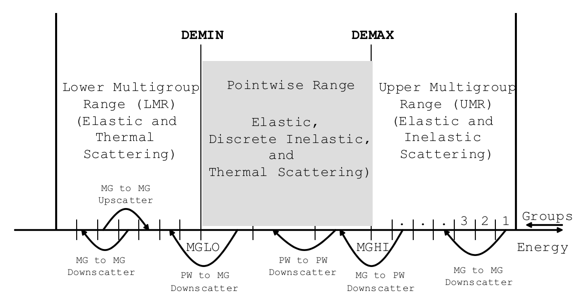
Fig. 7.4.1 Definition of UMR, PW, and LMR energy ranges.
Several transport computation methods are available for both MG and PW calculations. These include a space-independent slowing down calculation for infinite homogeneous media, 1D discrete ordinates or P1 methods for slab, spherical, and cylindrical geometries, and a 2D method of chracateristics (MoC) method for lattice unit cells. A simplified two-region collision-probablity method is also available for ther pointwise solution. In general the user may specify different transport methods for the UMR, PW, and LMR, respectively; however, if the 2D MoC method is specified for any range, it will be used for all.
The CENTRM 1D discrete ordinates calculation option has many of the same features as the SCALE MG code XSDRNPM. It represents the directional dependence of the angular flux with an arbitrary symmetric-quadrature order, and uses Legendre expansions up to P5 to represent the scattering source. No restrictions are placed on the material arrangement or the number of spatial intervals in the calculation, and general boundary conditions (vacuum, reflected, periodic, albedo) can be applied on either boundary of the 1D geometry. Lattice cells are represented in the CENTRM discrete ordinates option by a 1D Wigner-Sitz cylindrical or spherical model with a white boundary condition on the outer surface.
Starting with SCALE-6.2, CENTRM also includes a 2D MoC solver for lattice cell geometries consisting of a cylindrical fuel rod (fuel/gap/clad) contained within a rectangular moderator region. The MoC calculation is presently limited to square lattices. The 2D unit cell uses a reflected boundary condition on the outer square surface, which provides a more rigorous treatment than the 1D Wigner-Seitz model; however the MoC option requires a longer execution time than the 1D discrete ordinates method. The MoC option has been found to improve results compared to the 1D Wigner-Seitz cell model for many cases, but in other cases the improvement is marginal.
A variable PW energy mesh is generated internally to accurately represent the fine-structure flux spectrum for the system of interest. This gives CENTRM the capability to rigorously account for resonance interference effects in systems with multiple resonance absorbers. Because CENTRM calculates the space-dependent PW flux spectrum, the spatial variation of the self-shielded cross sections within an absorber body can be obtained. A radial temperature distribution can also be specified, so that space-dependent Doppler broadening can be treated in the transport solution. Within the epithermal PW range, the slowing-down source due to elastic and discrete-level inelastic reactions is computed with the analytical scatter kernel based upon the neutron kinematic relations for s-wave scattering. Continuum inelastic scatter is approximated by an analytical evaporation spectrum, assumed isotropic in the laboratory system. For many thermal reactor and criticality safety problems, self-shielding of inelastic cross sections has a minor impact, and by default these options are turned off for faster execution. As previously discussed, the thermal scatter kernel is based on the ENDF/B scattering law data for bound moderators, and uses the free-gas model for other materials.
7.4.2. Theory and Analytical Models
This section describes the coupled MG and PW techniques used to solve the neutron transport equation.
7.4.2.1. Energy/lethargy ranges for MG and PW calculations
The combined MG/PW CENTRM calculation is performed over the energy range spanned by the group structure in the input MG library. The energy boundaries for the “IGM” neutron groups specified on the MG library divide the entire energy range into energy intervals. The lowest energy group contained in the UMR is defined to be “MGHI”; while the highest energy group in the LMR is designated “MGLO.” The boundary between the PW and UMR energy intervals is set by the energy value “DEMAX,” while “DEMIN” is the boundary between the PW and LMR. The default values of 0.001 eV and 20 keV for DEMIN and DEMAX, respectively, can be modified by user input, but the input values are altered by the code to correspond to the closest group boundaries. Hence, DEMAX is always equal to the lower energy boundary of group MGHI and DEMIN the upper energy boundary of MGLO. The PW calculation is performed in terms of lethargy (u), rather than energy (E). The origin (u=0) of the lethargy coordinate corresponds to the energy E=DEMAX, which is the top of the PW range. See Fig. 7.4.2.
The highest energy group of the thermal range is defined by the parameter “IFTG,” obtained from the MG library. If DEMIN is less than the upper energy boundary of IFTG, the PW range extends into thermal. In this case, scattering in the PW region of the thermal range is based on the PW scattering kernel data; and the LMR calculation uses 2D transfer matrices for incoherent and coherent scattering on the MG library. Coupling between the MG and PW thermal calculations is treated, and outer iterations are required to address effects of upscattering.

Fig. 7.4.2 Definition of High and Transition regions in upper multigroup region.
With the exception of hydrogen moderation, elastic down-scattering coupling the UMR and PW ranges, occurs only within a limited sub-range of the UMR called the “transition region”. The highest energy group in the transition region is designated “MGTOP.” The precise definition of the transition region is given in Sect. 7.4.2.6.1.
Energy boundaries of the group structure on the input MG library correspond to the IGM+1 values, { G1, G2, … Gg, Gg+1, …, GIGM+1}. It is convenient to designate the number of groups in the UMR, PW, and LMR ranges equal to NGU, NGP, and NGL, respectively, so that IGM = NGU + NGP + NGL; or in terms of the parameters MGHI and MGLO introduced previously:
NGU = MGHI; NGP = MGLO - MGHI - 1; NGL = IGM - MGLO + 1.
The flux per unit lethargy is calculated for a discrete energy (or lethargy) mesh spanning the MG structure. Groups in the UMR and LMR each contain a single energy mesh point, while groups in the PW range generally contain several points. The number of mesh points in the UMR, PW, and LMR is equal respectively to NGU, NP, and NGL; and the total number of points in the entire energy mesh is designated as “NT,” which is equal to NGU + NP + NGL. Thus the lethargy (u) mesh consists of the set of points: {u:sub:1,….uNGU, uNGU+1,….uNGU+NP, uNGU+NP+1,…uNT}. Based on the lethargy origin at E=DEMAX, the lethargy “un” associated with any energy point “En” is equal to,
un = ln(DEMAX/En).
Lethargy points are arranged in order of increasing value. The lethargy origin is at point NGU+1, the lower energy boundary of group MGHI; i.e., uNGU+1=0. Note that the entire UMR (E>DEMAX) corresponds to negative lethargy values. Lethargy values for the first NGU and the last NGL points in the mesh are defined to be the midpoint lethargies of groups in the UMR and LMR ranges, respectively. For example, for the NGU groups within the UMR,
u1 = 0.5[ln(DEMAX/G1) + ln(DEMAX/G2)];
uNGU = 0.5[ln(DEMAX/GMGHI) + ln(DEMAX/GMGHI + 1)];
and similarly for the NGL groups in the LMR,
uNGU + NP + 1 = 0.5[ln(DEMAX/GMGLO) + ln(DEMAX/GMGLO + 1)]
uNT = 0.5[ln(DEMAX/GIGM) + ln(DEMAX/GIGM + 1)]
The remaining NP points in the mesh (i.e., values uNGU+1 to uNGU+NP) are contained within the NGP groups that span the PW range. By definition the first point in the PW range is the lower energy boundary of group MGHI. The other mesh points are computed internally by CENTRM, based on the behavior of the macroscopic PW total cross sections and other criteria.
The neutron flux, as a function of space and direction, is calculated for each energy/lethargy point in the mesh by solving the Boltzmann transport equation. The transport equation at each lethargy point generally includes a source term representing the production rate due to elastic and inelastic scatter from other lethargies, which couples the solutions at different lethargy mesh points. Except in the thermal range, neutrons can only gain lethargy (lose energy) in a scattering reaction; thus the PW flux is computed by solving the transport equation at successive mesh points, sweeping from low to high lethargy values.
7.4.2.2. The Boltzmann equation for neutron transport
The steady state neutron transport equation shown below represents a particle balance-per unit phase space, at an arbitrary point :math:` ho` in phase space,
where:
\(\psi\left(\rho \right)\) = angular flux (per lethargy) at phase space coordinate \(\rho\);
\(\rho = \left(r,u,\Omega \right)\) = phase space point defined by the six independent variables;
r = (x1,x2,x3) = space coordinates;
u = ln( Eref /E) = lethargy at energy E, relative to an origin (u=0) at Eref;
\(\Omega\) = ( \(\mu\), \(\zeta\)) = neutron direction defined by polar cosine \(\mu\) and azimuthal angle \(\zeta\);
\(\Sigma_t\left(r, u \right)\) = macroscopic total cross section;
\(\Sigma\left(u^{\prime}\rightarrow u; \mu_0 \right)\) = double differential scatter cross section;
\(\mu_0\) = cosine of scatter angle, measured in laboratory coordinate system;
\(Q_{ext} \left( \rho \right)\) = external source term, including fission source;
The left and right sides of Eq. (7.4.1) respectively, are equal to the neutron loss and production rates, per unit volume-direction-lethargy. In CENTRM the spatial distribution of the fission source is input as a component of the external source Q; hence, a fixed source rather than an eigenvalue calculation is required for the transport solution.
The angular dependence of the double-differential macroscopic scatter cross section of an arbitrary nuclide “j” is represented by a finite Legendre expansion of arbitrary order L:
where \(P_{\ell} \left( \mu_0 \right)\) = Legendre polynomial evaluated at the laboratory scattering cosine \(mu_0\); and
\(\Sigma^{\left(j \right)}\left(u^{\prime} \rightarrow u\right)\) = cross section moments of nuclide j, defined by the expression
After substitution of the above Legendre expansions for the scattering data of each nuclide, and applying the spherical harmonic addition theorem in the usual manner, the scattering source on the right side of Eq. (7.4.1) becomes [CENTRM-BG70]:
wherein,
\(\mathrm{Y}_{\ell \mathrm{k}}(\Omega)=\mathrm{Y}_{\ell \mathrm{k}}(\mu, \zeta)\) = the spherical harmonic function evaluated at direction \(\Omega\)
\(\mathrm{S}_{\ell \mathrm{k}}\) = spherical harmonic moments of the scatter source, per unit letharagy.
The summation index \("\ell k"\) indicates a double sum over \(\ell\) and \(k\) indices; in the most general case it is defined as:
where “L” is the input value for the maximum order of scatter (input parameter “ISCT”).
Due to symmetry conditions, some of the source moments may be zero. The parameter LK is defined to be the total number of non-zero moments (including scalar flux) for the particular geometry of interest, and is equal to,
LK = L + 1 for 1D slabs and spheres;
LK = L*(L+4)/4+1 for 1D cylinders, and
LK = L*(L+3)/2+1 for 2D MoC cells
More details concerning the 1-D Boltzmann equation can be found in the XSDRNPM chapter of the SCALE manual.
7.4.2.3. Legendre moments of the scattering source
The \(S_{\ell k}\) moments in Eq. (7.4.4) correspond to expansion coefficients in a spherical harmonic expansion of the scatter source. These can be expressed in terms of the cross section and flux moments by
where \(\psi_{\ell k}= \left(u\right)\) = spherical harmonic moments of the angular flux;
and \(S_{\ell k}^{\left(j \right)} \left(u^{\prime} \rightarrow u \right)\) = moments of the differential scatter rate from lethargy u\(\prime\) to u, for nuclide “j”;
The \(\psi_{\ell k}\) flux moments are the well known coefficients appearing in a spherical harmonic expansion of the angular flux. These usually are the desired output from the transport calculation. In particular, the \(\ell=0\), \(k=0\) moment corresponds to the scalar flux [indicated here as \(\phi\left( r,u\right )\)],
In general the epithermal component of the scatter source in Eq. (7.4.4) contains contributions from both elastic and inelastic scatter reactions; however, inelastic scatter is only possible above the threshold energy corresponding to the lowest inelastic level. The inelastic Q values for most materials are typically above 40 keV; therefore, elastic scatter is most important for slowing down calculations in the resolved resonance range of most absorber materials of interest. For example, the inelastic Q values of 238U, iron, and oxygen are approximately 45 keV, 846 keV, and 6 MeV, respectively; while the upper energy of the 238U resolved resonance range is 20 keV in ENDF/B-VII. The inelastic thresholds of some fissile materials like 235U and 239Pu are on the order of 10 keV; however, with the exception of highly enriched fast systems, these inelastic reactions usually contribute a negligible amount to the overall scattering source. CENTRM assumes that continuum inelastic scatter is isotropic in the laboratory system, while discrete level inelastic scatter is isotropic in the center of mass (CM) coordinate system.
Over a broad energy range, elastic scatter from most moderators can usually be assumed isotropic (s-wave) in the neutron-nucleus CM coordinate system. In the case of hydrogen, this is true up to approximately 13 MeV; for carbon up to 2 MeV; and for oxygen up to 100 keV. However, it is well known that isotropic CM scatter does not result in isotropic scattering in the laboratory system. For s-wave elastic scatter the average scatter-cosine in the laboratory system is given by: \(\bar{\mu}_{0}=0.667 / \mathrm{~A};^{3}\) where “A” is the mass number (in neutron mass units) of the scattering material. This relation indicates that s-wave, elastic scattering from low A materials tends to be more anisotropic in the laboratory, and that the laboratory scattering distribution approaches isotropic \(\left(\bar{\mu}_{0}=0 ; \theta_{0}=90\right)\) as A becomes large. For example, the \(\bar{\mu}_{0}\) of hydrogen is 0.667 (48.2°); while it is about 0.042 (87.6°) for oxygen. Because s-wave scattering from heavy materials is nearly isotropic in the laboratory system, the differential scattering cross section (and thus the scattering source) can usually be expressed accurately by a low order Legendre expansion. On the other hand light moderators like hydrogen may require more terms-depending on the flux anisotropy-to accurately represent the elastic scatter source in the laboratory system. The default settings in CENTRM are to use P0 (isotropic lab scatter) for mass numbers greater than A=100, and P1 for lighter masses.
An analytical expression can be derived for the cross-section moments in the case of two-body reactions, such as elastic and discrete-level inelastic scattering from “stationary” nuclei. Stationary here implies that the effect of nuclear motion on neutron scattering kinematics is neglected.
Note
The stationary nucleus approximation for treating scattering kinematics does not imply that the effect of nuclear motion on Doppler broadening of resonance cross sections is ignored, since this effect is included in the PW cross-section data.
In CENTRM the stationary nucleus approximation is applied above the thermal cutoff, typically around 3-5 eV, but is not valid for low energy neutrons. CENTRM has the capability to perform a PW transport calculation in the thermal energy range using tabulated thermal scattering law data for bound molecules, combined with the analytical free-gas kernel for other materials. In this case the cross-section moments appearing in Eq. (7.4.3) include upscattering effects. The expressions used in CENTRM to compute the PW scatter source moments in the thermal range are given in Sect. 7.4.2.6.
The following two sections discuss the evaluation of the scatter source moments for epithermal elastic and inelastic reactions, respectively.
7.4.2.3.1. Epithermal Elastic Scatter
Consider a neutron with energy E\(\prime\), traveling in a direction \(\Omega\)\(\prime\), that scatters elastically from an arbitrary material “j,” having a mass A(j) in neutron-mass units. Conservation of kinetic energy and momentum requires that there be a unique relation between the angle that the neutron scatters (relative to the initial direction) and its final energy E after the collision. If the nucleus is assumed to be stationary in the laboratory coordinate system, then the cosine (μ0) of the scatter angle (\(\theta\)0) measured in the laboratory system, as a function of the initial and final energies, is found to be
where the kinematic correlation function G relating E\(\prime\), E, and μ0 for elastic scatter is equal to
The final energy E of an elastically scattered neutron is restricted to the range,
where \(\alpha^{(j)}\) = maximum fractional energy lost by elastic scatter
The corresponding range of scattered neutrons in terms of lethargy is equal to
where
The double-differential scatter kernel of nuclide j (per unit lethargy and solid angle) for s-wave elastic scatter of neutrons from stationary nuclei, is equal to
The presence of the Dirac delta function completely correlates the angle of scatter and the values of the initial and final energies. Substituting the double differential cross-section expression from Eq. (7.4.16) into Eq. (7.4.3) gives the single-differential Legendre moments of the cross section, per final lethargy:
where \(P_{\ell}\) = Legendre polynomial evaluated at argument G(j) equal to the scatter cosine.
When the above expressions are used in Eq. (7.4.6), the following is obtained for the \(\ell k\) moment of the epithermal elastic scattering source at lethargy u:
7.4.2.3.2. Epithermal Inelastic Scatter
If the input value of DEMAX is set above the inelastic threshold of some materials in the problem, then inelastic scattering can occur in the PW range. The pointwise transport calculation may optionally include discrete-level and continuum inelastic reactions in computing the PW scatter source moments. The multigroup calculations always consider inelastic reactions.
Discrete-level inelastic reactions are two-body interactions, so that kinematic relations can be derived relating the initial and final energies and the angle of scatter. It can be shown that the kinematic correlation function for discrete-level inelastic scatter can be written in a form identical to that for elastic scatter by redefining the parameter a1 in Eq. (7.4.11) to be the energy dependent function [CENTRM-Wil00],
The parameter Q(m, j) is the Q-value for the mth level of nuclide “j”. The Q value is negative for inelastic scattering, while it is zero for elastic scatter. The threshold energy in the laboratory coordinate system is proportional to the Q-value of the inelastic level, and is given by:
The range of energies that can contribute to the scatter source at E, due to inelastic scatter from the mth level of nuclide j is defined to be [E:sub:L , E:sub:H], where EH >E:sub:L >E:sub:T. This energy range has a corresponding lethargy range of [u:sub:LO , u:sub:HI] which is equal to,
The energy-dependent alpha parameters in the above expressions are defined as,
where
Modifying the epithermal elastic scatter source in Eq. (7.4.18) to include discrete-level inelastic scatter gives the following expression
Detailed expressions for the lethargy limits are given in [CENTRM-Wil00]. Since \(\Delta^{\left( m,j\right)}\) is equal to unity for elastic scatter, the above equation reduces to Eq. (7.4.15) if there is no discrete-level inelastic contribution.
At high energies, the inelastic levels of the nucleus become a continuum. In this case CENTRM represents the energy distribution of the scattered neutrons by an evaporation spectrum with an isotropic angular distribution in the lab system; thus, only the P0 moment appears in the continuum inelastic scattering source. Including continuum inelastic reactions in the PW calculation usually has a small impact on the spectrum used for resonance self-shielding, and may adversely impact the computer memory requirements and execution time. Therefore, by default, CENTRM does not include continuum inelastic reactions in the pointwise solution; however, it is always included in the UMR solution.
7.4.2.3.3. Thermal Scatter
Since thermal neutrons have energies comparable to the mean kinetic energy of molecules in thermal equilibrium, the scattering kernels must account for molecular motion. The scatter moments include both downscatter as well as upscatter contributions; hence, the integration limits appearing in Eq. (7.4.18) must be extended from the lowest to the highest energy of the thermal range. Furthermore the cross-section moments correspond to the Legendre expansion coefficients of the thermal scatter kernel, which has a substantially different form than the epithermal kernel discussed in the previous two sections. In general the \(\ell^{\mathrm{th}}\) Legendre moment of the thermal scattering kernel at temperature T, describing scattering from \(E\) to \(E^{\prime}\), is given by
where \(\beta\left(E^{\prime} \rightarrow E \right)\) and \(\alpha \left(E^{\prime},E,\mu_0 \right)\) are dimensionless variables (functions of temperature) defining the energy and momentum exchange, respectively, of the collision [CENTRM-BG70]; \(\sigma\)b is the rigidly bound scatter cross section, which is proportional to the free atom cross section; and S(\(\alpha\), \(\beta\); T) describes the temperature-dependent thermal scattering law.
If atomic bonding effects are neglected, the atoms of a material behave like a gas in thermal equilibrium at the temperature of the medium. In this case S(\(\alpha\), \(\beta\)) can be expressed by an analytical function. CENTRM uses the free gas model for all nuclides except those materials that have thermal scattering laws available in the ENDF/B nuclear data files. The ENDF/B scattering law data account for the effects of molecular bonding and possible polyatomic crystalline structure. While free-gas kernels are computed internally in CENTRM, the kernel moments describing bound thermal scatterers are stored in a data file that can be accessed by CENTRM.
7.4.2.3.4. Bound thermal kernels
Thermal scattering from bound atoms is classified either as an “inelastic reaction,” in which the neutron energy may change, or an “elastic reaction,” in which the neutron changes direction, but does not change energy. In ENDF/B the former reactions are treated as incoherent inelastic scattering with a doubly differential kernel describing the secondary neutron energy and angle distribution. The latter reactions are usual treated as coherent elastic scatter characterized by diffractive interference of the scattered deBroglie waves, although a few materials are modeled by the incoherent elastic approximation. Legendre moments for thermal elastic kernels describe the secondary angular distribution with no energy exchange, at a given neutron energy. Bound scatter kernels have been processed by the AMPX code system for most of the ~25 compounds with thermal scatter laws in ENDF/B, and are stored in individual kinematics files distributed with the SCALE code system. These include materials such as: H in water, H and C in polyethylene, H and Zr in ZrH, C in graphite, deuterium in heavy water, Be metal, Be in BeO, etc. The CRAWDAD module processes scattering kernel data for individual nuclides into a combined library used in CENTRM, and also interpolates the kernels to the appropariate temperatures.
The bound scatter kernels are tabulated at different energy points from the flux solution mesh; therefore it is necessary to map the data onto the desired energy mesh in the CENTRM calculation. Because thermal elastic scattering results in no energy loss, the elastic moments only appear in the within-point term of the scattering source in the CENTRM thermal calculation. Thus the coherent elastic data is easily interpolated since it only involves a single energy index and temperature. However, the incoherent inelastic moments are 2-D arrays in terms of the initial and final energies, so that a 2-D interpolation must be done for each temperature. CENTRM uses a simple type of “unit-base transform” method to interpolate incoherent inelastic kernels onto the flux solution mesh. The method attempts to preserve the absolute peak of the secondary energy distribution, at given initial energy. For water-bound hydrogen and several other moderators, this is quite adequate, since the kernel generally has only a single maximum. However, if more than one local extrema is present, such as for graphite, the other local peaks are not explicitly preserved in the interpolation method. For this reason it is necessary to include a fairly dense set of initial energies in the tabulated kernels of graphite and similar materials, to avoid gross changes in the kernel shape at adjacent initial energy panels.
7.4.2.3.4.1. Free gas thermal kernels
CENTRM computes free-gas kernels using the approach proposed by Robinson [CENTRM-Rob81] as a modification to the original FLANGE [CENTRM-HF71] methodology. Legendre moments of the free-gas scatter kernel per unit lethargy are expressed as,
where \(W_{\ell n}\) are constant coefficients associated with the Legendre polynomial of order \(\ell\); \(\Sigma_{free}\) is the constant free-atom cross section for the material; and Hn are the \(\alpha\)-moments of the free-gas scatter law, given as
The limits on the above integral correspond to:
The alpha moments for n > 0 can be evaluated very efficiently using a recursive relation [CENTRM-Wil00]:
where Fn is the function,
Analytical expressions for the initial two moments, H0 and H:sub:` -1`, are given in [CENTRM-Rob81].
The standard free-gas kernel is based on the assumption of a constant free atom cross section. When averaged over the molecular velocity distribution, this gives a 1/v variation in the effective free-gas cross section at low energies. To approximately account for nuclear structure effects on the energy dependence of the thermal cross section (e.g., low energy resonances), the free-gas moments are multiplied by the ratio \(\sigma\)s(E)/\(\sigma\)FG(E), where \(\sigma\)s is the Doppler broadened scatter cross section processed from ENDF/B data; and \(\sigma\)FG is the effective free-gas cross section,
where \(\mathrm{y}^{2}=\mathrm{~A} \frac{\mathrm{E}}{\mathrm{kT}}\).
7.4.2.4. Sub-moment expansion of the epithermal scattering source
One difficulty in computing the epithermal scatter source moments is that the Legendre polynomial in the integrand of Eq. (7.4.18) and Eq. (7.4.24) is a function of both the initial and final lethargy (or energy) of the scattered neutrons, due to the correlation function \(G^{\left(j \right)} \left(E,E^{\prime} \right)\)). At each lethargy u this requires that the \(u^{\prime}\)-integral be recomputed over all lower lethargies, for every nuclide and moment. A more efficient algorithm would be possible if the differential scattering moments appearing in the integrand could be factored into a product of a function of u multiplied by a function of \(u^{\prime}\) such as
where F and H are the two factors (to be specified later).
If this is done, the u-function can be factored from the scatter source integrals, leaving only integrals over the u\(\prime\)-function as shown below:
Because the factored integrand does not depend on the variable u, a running summation over all \(u^{\prime}\) points can be accumulated and saved as the calculation sweeps from low to high lethargy. For example, note that the \(\ell=0\) moment in Eq. (7.4.18) is already separable into a product of u times \(u^{\prime}\) because P0 is equal to one at all values of G. Thus the isotropic component of the elastic differential scatter rate (per unit lethargy) from \(u^{\prime}\) to u is proportional to E/E^{prime}, where
Therefore, the two separable factors in the lowest moment, \(S^{\left( j \right)}_{0.0} \left( u^{\prime} \rightarrow u \right)\) are identified as,
However, the higher order Legendre moments contain the term \(P_{\ell} \left( G \right)\) in the integrand; and the expression for \(G\left(E^{\prime},E \right)\) is a difference of two terms that depend on both E and \(E^{\prime}\). A new method called a “sub-moment expansion” has been developed for CENTRM that allows the Legendre polynomials appearing in the differential scatter moments to be factored into the desired separable form. Each spherical harmonic moment of the scattering source appears expanded in a series of factored “sub-moments.”
The Legendre polynomial of order \(\ell\) is a polynomial containing terms up to the \(ell^{\mathrm{th}}\) power. Applying the binomial expansion theorem and some algebraic manipulation, the standard expression for \(P_{\ell}\) evaluated at “G” can be expressed as
where \(h_k \left(E \right) = E^{1+K/2}\); and the expansion coefficients \(\tilde{\mathrm{g}}_{\ell, \mathrm{k}}\) are equal to, \(\tilde{\mathrm{g}}_{\ell \mathrm{K}}=\frac{\mathrm{g}_{\ell \mathrm{K}}}{N_{\ell} \times \alpha_{1}^{\ell}}\) where the \(g_{\ell,K}\) (no tilde) parameters were defined in [CENTRM-WA95] to be:
In Eq. (7.4.36)-Eq. (7.4.37), the constants \(b_{m,\ell}\) and \(N_{\ell}\) are the standard Legendre constants and normalization factors, respectively, which are tabulated in Table 7.4.1 for orders through P7; and \(\left(\begin{array}{c} \mathrm{m} \\ \mathrm{i} \end{array}\right)=\) the binomial expansion coefficients(20) \(= \frac{\mathrm{m} !}{(\mathrm{m}-\mathrm{i}) ! \quad \mathrm{i} !}\)

|
The explicit dependence of the constants a1 and a2 on the nuclide index j [see Eq. (7.4.11)] has been suppressed to simplify notation. For discrete-level inelastic scatter the parameter a1 is an energy dependent function given by Eq. (7.4.19), but for elastic scatter this reduces to the constant in Eq. (7.4.11). Note that the \(g_{\ell,K}\) value is zero unless \(\ell\) and K are both even or both odd, respectively, so that about half the terms appearing in the summation of Eq. (7.4.36) vanish. Table 7.4.2 through Table 7.4.4 give values for the submoment expansion coefficients for several nuclides.
The sub-moment expansion of the scattering source, including both elastic and discrete-level inelastic reactions, is obtained by substituting the expansion of the Legendre polynomial from Eq. (7.4.36) into Eq. (7.4.26), giving
where \(Z_{\ell \mathrm{K}}^{(\mathrm{m}, \mathrm{j})}(E)=a_{1}^{\ell}(E) \frac{\tilde{g}_{\ell, K}^{(m, j)}(E)}{\left(1-\alpha^{(j)}\right)}\). For elastic scatter, the Z coefficients are independent of energy.
With this approach the scatter source moments in Eq. (7.4.39) have been further expanded into a summation of “submoments” identified by index K (although some of these terms are equal to zero, due to the behavior of the \(g_{\ell,K}\) coefficients). Each term has the desired factored form expressed in Eq. (7.4.32); i.e., separable in terms of the variables u and \(u^{\prime}\) with
so that the lkth moment of the scatter source can be written as
7.4.2.4.1. Characteristics and Properties of the Sub-Moment Expansion
The expansion in Eq. (7.4.36) becomes numerically unstable for heavy nuclides (large A), with high Legendre orders. Using double precision arithmetic, it was found that the accuracy of the expansion begins to break down for heavy nuclides (A100) if the order of scatter exceeds P5; although the expansion for lighter nuclides (viz, moderators) is very accurate even for scattering orders as high as P7 or more. For this reason CENTRM has an option to restrict the Legendre expansion to lower orders for heavy masses, while using the input value of “ISCT” for lighter nuclides. The restricted Legendre order and mass cut-off value can be controlled by user input, but the default is P0 (i.e., isotropic lab scattering) for A>100. Table 7.4.5 shows the maximum error observed in the series representation of Legendre polynomials up to P5, for selected mass numbers. These values were obtained by evaluating the series expansion for \(P_{\ell} \left( G \left(x \right) \right)\) in Eq. (7.4.36), and comparing to the exact value computed at 11 equally spaced values for \(E/E^{\prime}\). The observed error in the P5 polynomial expansion is < 1% even for heavy materials such as 238U, while nuclides whose mass is < 100 are computed nearly exactly by the expansion.
Although the accuracy of the submoment expansion is good through P7 scattering in moderators, Legendre expansions above P3 are not recommended because the number of terms in the expansion increases rapidly with increasing scattering order, especially for 2D MoC and 1D cylindrical systems. The number of spherical harmonic moments appearing in the scattering source depends on the order (L=ISCAT) of the Legendre expansion used to represent the differential scatter cross section, as well as on the type of geometry (slab, spherical, cylindrical, or 2D MoC) used in the transport calculation. The submoment method further expands each source moment. Table 7.4.6 shows the number of moments in the cross-section expansion, and the number of moments and submoments in the scatter source expansion, as a function of scatter order and geometry type. Although the use of cumulative integrals discussed below allows the sub-moments to be evaluated rapidly, the large number of terms becomes prohibative for high scattering orders. Fortunately a P1 Legendre order is sufficient for most self-shielding calculations, and orders beyond P2 should seldom be required for reactor physics and criticality applications.
\(\tilde{g}_{1, K} \quad, \quad \mathrm{~K}=-1, \ldots, 1\) |
||||||||
|---|---|---|---|---|---|---|---|---|
Legendre order (\(\ell\)) |
K: |
-3 |
-2 |
-1 |
0 |
1 |
2 |
3 |
0 |
1 |
|||||||
1 |
0 |
0 |
1 |
|||||
2 |
0 |
0 |
-0.5 |
0 |
1.5 |
|||
3 |
0 |
0 |
0 |
-1.5 |
0 |
2.5 |
||
*For A=1, \(\mathrm{G}(\mathrm{x})=\mathrm{x} ;\left[\mathrm{x}=\left(\mathrm{E} / \mathrm{E}^{\prime}\right)^{1 / 2}\right.\); where E’,E=initial and final energies. |
||||||||
\(\tilde{g}_{l, K} \quad, \quad \mathrm{~K}=-1, \ldots, 1\) |
||||||||
Legendre order (\(\ell\)) |
K |
-3 |
-2 |
-1 |
0 |
1 |
2 |
3 |
0 |
1 |
|||||||
1 |
-0.88235294 |
0 |
1 |
|||||
2 |
1.16782007 |
0 |
-2.6539724 |
0 |
1.5 |
|||
3 |
-1.7173824 |
0 |
5.85741909 |
0 |
-6.6384083 |
0 |
2.5 |
|
*For A=16, \(\mathrm{G}(\mathrm{x})=\frac{8.5}{\mathrm{x}}-7.5 \mathrm{x}:\left[\mathrm{x}=\left(\mathrm{E} / \mathrm{E}^{\prime}\right)^{1 / 2}\right.\); where E’,E=initial and final energies. |
||||||||
\(\tilde{g}_{1, K} \quad, \quad \mathrm{~K}=-1, \ldots, 1\) |
||||||||
|---|---|---|---|---|---|---|---|---|
Legendre order (\(\ell\)) |
K |
-3 |
-2 |
-1 |
0 |
1 |
2 |
3 |
0 |
1 |
|||||||
1 |
-0.99156118 |
0 |
1 |
|||||
2 |
1.47479036 |
0 |
-2.97471915 |
0 |
1.5 |
|||
3 |
-2.43724146 |
0 |
7.37405774 |
0 |
-7.43681568 |
0 |
2.5 |
|
*For A=236, \(G(x)=\frac{118.5}{x}-117.5 x:\left[x=\left(E / E^{\prime}\right)^{1 / 2}\right.\); where E’,E=initial and final energies. |
||||||||
Legendre order (\(ell\)) |
Mass number in neutron mass units (A) |
|||||
|---|---|---|---|---|---|---|
1 |
12 |
56 |
100 |
150 |
236 |
|
1 |
0(*) |
0 |
0 |
0 |
0 |
0 |
2 |
0 |
0 |
0 |
0 |
0 |
0 |
3 |
0 |
0 |
0 |
0 |
0 |
0 |
4 |
0 |
0 |
0 |
0 |
0 |
1.2 \(\times\) 10-5 |
5 |
0 |
0 |
0 |
2.1 \(\times\) 10-5 |
3.9 \(\times\) 10-3 |
8.4 \(\times\) 10-3 |
(*) 0 error indicates \(< 10^{-6}\). |
||||||

|
7.4.2.4.2. Scattering moments expressed with cumulative integral operator
It will be convenient to express the scatter source moments in terms of an integral operator \(\mathbb{C}\), designated here as the “cumulative integral.” The domain of this operator is the vector space of all integrable lethargy functions. The operator is defined for an arbitrary domain element \(f\left( u^{\prime} \right)\), at an arbitrary lethargy limit U, to be:
where u0 is an arbitrary reference point. In implementing this method in CENTRM, it is convenient to set u0=uL; i.e., the negative lethargy value corresponding to highest energy of the transition range.
The cumulative integral at some lethargy mesh point un is related to the value at the previous lethargy mesh point un-1 by the expression
where un > un-1.
Note that only a single panel of integration over the interval [un-1, un] must be performed to update the cumulative integrals.
The sub-moment expansion of the scatter source in Eq. (7.4.38) can be expressed in terms of the cumulative integral operator as follows:
For elastic scatter the value of \(\mathrm{u}_{\mathrm{LO}}^{(\mathrm{m}, \mathrm{j})}\) is equal to \(u-\varepsilon^{\left( j \right)}\), and \(\mathrm{u}_{\mathrm{HI}}^{(\mathrm{m}, \mathrm{j})}\) is equal to u.
7.4.2.5. Multigroup Boltzmann equation
The MG form of the transport equation used in the UMR and LMR is derived by integrating Eq. (7.4.1) over the energy intervals defined by the group structure in the MG library. Details concerning the MG transport equation, including its solution using the discrete ordinates method, can be found in the SCALE documentation of XSDRNPM. The CENTRM MG solution is similar to the XSDRNPM method: however; the outer iteration loop in CENTRM is limited to the thermal groups, since no eigenvalue calculation is performed in CENTRM. The MG scatter source in the thermal range has upscatter contributions that depend on group fluxes from lower energy groups in the LMR, so that outer iterations are performed over thermal groups in the LMR until the upscatter portion of the MG scatter source converges.
7.4.2.5.1. Multigroup data for CENTRM calculation
Group cross-section data for the MG calculations are taken from the input MG library which should include a combined 2D transfer matrix representing all pertinent scatter reactions (viz, elastic, inelastic, coherent and incoherent thermal reactions, n-2n, etc). MG cross sections also should be problem-dependent values. This is done by processing the data with BONAMI prior to the CENTRM calculation. BONAMI converts the problem-independent cross-sections into problem-dependent values by using the Bondarenko factors on the MG library.
7.4.2.5.2. Conversion of multigroup fluxes to pseudo-pointwise values
The MG flux solution provides the integrated flux over lethargy, for each group interval. The average flux within a group is assumed to approximate the value of the flux per unit lethargy at the midpoint lethargy of the group; thus a set of “pseudo-pointwise” angular fluxes and moments can be obtained for the NGU and NGL mesh points in the UMR and LMR, respectively. For lethargy point un , corresponding to the midpoint lethargy of group g contained within the LMR and UMR, a PW flux value is computed from the expression,
where \(\Delta\)ug is the lethargy width of group g. Eq. (7.4.44) provides PW flux values for lethargy mesh points,
A linear variation of the flux per unit lethargy is assumed between lethargy points to obtain a continuous representation in the UMR and LMR.
7.4.2.6. The Boltzmann equation within the PW range
In contrast to the “pseudo-pointwise” fluxes obtained from the MG transport calculation, a true PW solution is performed for the NP lethargy points between DEMAX and DEMIN. The PW solution is performed within a loop over energy groups: i.e., for each of the NGP groups in the PW range there is an additional loop over all lethargy mesh points contained inside the group. This approach facilitates coupling of the scatter source from the UMR to the PW range and from the PW and LMR.
Evaluating Eq. (7.4.1) at each of the NP energy mesh-points in the PW range gives a system of integro-differential equations that can be solved to obtain the PW flux moments, per lethargy, for the NP energy mesh points in the range DEMAX to DEMIN-which correspond to the lethargy points, \(\mathrm{U}_{\mathrm{NGU}+1}, \ldots \mathrm{U}_{\mathrm{NGU}+\mathrm{NP}}\). Again linear variation of the flux between lethargy points is assumed, to obtain a continuous spectrum. Substituting Eq. (7.4.4) into Eq. (7.4.1), the PW transport equation at mesh point n is found to be,
for \(\mathrm{n}=\left(\mathrm{NG}_{\mathrm{U}}+1\right), \ldots .,\left(\mathrm{NG}_{\mathrm{U}}+\mathrm{N}_{\mathrm{P}}\right)\)
where
Aside from the definition of the cross-section data, the above equation appears identical in form to the MG transport equation, and can be solved with virtually the same algorithm as the MG solution, once the scatter source moments are determined. The same computer routines in CENTRM calculate both the MG and PW fluxes. However, a major conceptual difference between the PW and MG transport equations is that the PW equation describes a differential neutron balance per unit lethargy at an energy point, while the MG equation represents an integral balance over an interval of lethargy points. Although this type of point solution is not inherently conservative over the intervals defined by the energy mesh, the particle balance for each interval has been found to be very good. It should also be noted that exact particle conservation is not a strict requirement for this type of application where flux spectra rather than particle balances are primarily of interest.
In the PW range the scatter source is composed of (a) MG-to-PW scatter from the UMR and possibly upscatter from the LMR if the PW range extends into thermal, and (b) PW-to-PW scatter from points in the PW range. The submoment expansion method described previously is used in CENTRM to provide an efficient method of evaluating the PW-to-PW downscatter source for the epithermal range, which includes most of the resolved resonances.
7.4.2.6.1. Scattering sources for the PW range
In the case of elastic scatter from nuclide “j,” only the lethargy interval below \(u_n - \varepsilon^{\left( j \right)}\) can scatter to a lethargy point \(u_n\) in the PW range. If \(u_n - \varepsilon^{\left( j \right)}\) is negative, then some portion of the source at \(u_n\) is due to UMR-to-PW from energies above DEMAX, since zero-lethargy is equal to the top energy of the PW range. Otherwise, the elastic source is entirely PW-to-PW.
For any given nuclide j, the lowest lethargy in the UMR range that contributes to the elastic scatter source in the PW range is equal to \(-\epsilon^{\left( j \right)}\). Let “jL” represent the lightest non-hydrogen nuclide (i.e., having the smallest A value greater than unity) in the system. The associated fractional energy loss for this material is indicated as \(\alpha_L\), so that the highest energy neutron in the UMR range that can scatter into the PW range from an elastic collision with any non-hydrogenous moderator will have an energy equal to DEMAX/\(\alpha_L\). The corresponding lethargy is equal to be the negative value \(-\epsilon^{\left( L \right)}\), or -ln( \(\alpha_L\)). The value of \(-\epsilon^{\left( L \right)}\) is actually adjusted in CENTRM to coincide with the immediately preceding multigroup boundary, which has a lethargy value designated as uL. The interval of negative lethargy in the UMR between uL and 0 has been defined previously to be transition range, because the elastic slowing-down source from this interval provides a transition between the UMR and PW solutions, respectively. The transition range always contains an integer number of groups, corresponding to MGTOP to MGHI. The total downscatter source from the UMR to lethargy un is composed of elastic and inelastic contributions from the transition range between [uL,0]; and contributions from the “high” energy range from lethargies below uL. The high contribution comes from inelastic and hydrogen elastic reactions in the energy interval above the transition range.
The downscatter source at un in the PW range can thus be expressed as the sum of three distinct contributions - SHI, STr, and SPW -, that correspond to scatter from the high region of the UMR, the transition region of the UMR, and the PW ranges, respectively. The source moments appearing in Eq. (7.4.46) can thus be expressed as:
7.4.2.6.2. Downscatter source from high region of the UMR to the PW range (SHI)
The high region of the UMR corresponds to groups 1 through MGTOP-1. The MG-to-PW scattering source (SHI) from high energy region originates in the energy range above DEMAX/\(\alpha\)L; i.e., lethargies below uL (see Fig. 7.4.2). In this region, inelastic reactions may scatter neutrons to the PW range; but due to the definition of uL, the only elastic reactions that scatter to the PW range are due to hydrogen. Therefore in general, the MG matrices describing scatter from groups in high region to groups in the PW range correspond to discrete and continuum inelastic reactions, and elastic scatter from hydrogen. If \(g^{\prime}\) is an arbitrary group in the UMR range above the transition interval and g is a fixed group interval in the PW range, then the rate that neutrons scatter from all groups \(g^{\prime}\) in the high region to all energy points in g, for a given direction \(\Omega\), is obtained from the usual expression for MG-to-MG transfers, and is equal to
where MGLO > g > MGHI, and the MG source moments are,
while Eq. (7.4.50) gives the moments of the overall scatter rate from all groups in the high range into the entire PW group g, it is necessary to determine how the group source should be distributed over the PW energy mesh contained within the group; i.e., it is desired to extract the PW source moments, from the group moments by applying some “intra-group” distribution \(H_{\ell k,g} \left(E \right)\) such that,
The intra-group distribution has units of “per unit lethargy,” and its integral over the group is normalized to unity. This form of the scatter source preserves the MG moments \(S_{\ell k,g}\), whenever \(S_{\ell k, HI} \left( u \right)\) is integrated over group g, ensuring that the correct number of neutrons (as determined from the UMR calculation) will always be transferred from the high range into the PW group. Only the distribution within the group is approximate.
Recall that the scatter source of concern here is due only to elastic scatter from hydrogen and inelastic scatter from all other materials. In the case of s-wave elastic scatter from hydrogen, the P0 and P1 moments per unit lethargy, respectively, can be rigorously expressed in the form of Eq. (7.4.51) with
These expressions can be inferred directly from the moments of the scatter kernel in Eq. (7.4.17). The higher order scatter moments for hydrogen have a somewhat more complicated form containing sums of energy functions; but since these moments are usually less important than the first two moments, a less rigorous treatment of their intra-group distribution is used. The intra-group distribution due to inelastic scatter depends on the Q values for the individual levels, and these are not available on the multigroup libraries. Fortunately, the scatter source in the PW range is not very sensitive to the assumed intra-group distribution for inelastic scatter, as long as the total inelastic source for the group is computed correctly. As a reasonable trade-off between rigor and complexity, the high energy component of the UMR-to-PW scatter source is approximated using H0 for the intra-group distribution of all P0 moments, and H1 for all higher order moments. This approximation produces the correct intra-group variation for the lowest two moments of the hydrogen scatter source, but the higher order moments of hydrogen and the inelastic scatter source are not distributed exactly throughout the group. However, the integrated source moments are correct in all cases. Again, it should be emphasized that the approximations discussed here only apply to the UMR-to-PW component designated as SHI, which comes from reactions above the transition range (energies above \(E_{HI} / \alpha_L\)). This is often a small contribution to the overall PW source term.
7.4.2.6.3. Scattering sources from UMR transition region and epithermal PW range
Most coupling between the UMR and the PW range is due usually to elastic scatter from energies immediately above DEMAX. The contribution to the PW source due to downscatter source from this transition range has been designated STr(un). The other component of the PW source, SPW(un), accounts for the scattering source coming from all lethargies lower than un in the PW range. It is convenient to combine the two sources together as the PW epithermal source called “SEp,” which has an lkth moment given by Eq. (7.4.32),
This is done because CENTRM uses the submoment expansion technique to compute both the PW-to-PW epithermal source from the PW range as well as the MG-to-PW source from the transition range of the UMR. Note that elastic scattering from the transition range only impacts the PW scatter source at the initial mesh points in the PW range; i.e., those contained in the interval \(0 < u_n < \epsilon^{\left( j \right)}\), for nuclide j. Beyond these mesh points the elastic scatter source is due only to PW-to-PW scatter, as illustrated in Fig. 7.4.2.
The epithermal elastic source at un, coming from the range uL to un, is expressed as an integral over the immediately preceding lethargy mesh interval from un-1 to un plus the integral over the remaining lethargy interval, as illustrated in Fig. 7.4.3. The former integral is designated as I(un-1,un) and the latter as I(uL,un-1), so that
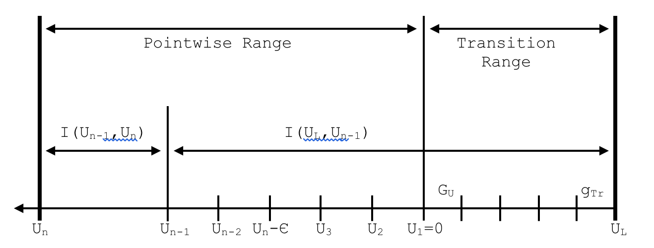
Fig. 7.4.3 Definition of cumulative integral elements.
The lethargy mesh in CENTRM is constrained such that the maximum lethargy gain in an elastic reaction (\(\epsilon^{\left(j \right)}\)) is always greater than the maximum mesh interval size, which insures that I(un-1,un) always includes the full panel from un-1 to un. In the above and subsequent equations the explicit dependence of SEp on independent variables other than lethargy is not shown for notational convenience. The integral I(un-1,un) is evaluated approximately by applying the trapezoidal rule, which leads to,
Using the submoment expansion from Eq. (7.4.38), Eq. (7.4.55) can be written for elastic scatter as
The first term on the right side of Eq. (7.4.56) corresponds to the “within-point” component of elastic scatter from un to un, which only occurs for straight ahead scatter (\(\mu_0=1\)). The within-point cross section is defined as,
In deriving this term the following relation has been used for each nuclide:
The I(uL,un-1) portion of the integral in Eq. (7.4.53) is equal to
Note that the lower lethargy limit of the integral is restricted to \(u_n - \epsilon^{\left( j \right)}\), since this is the maximum limit of lethargy that can scatter to un in an elastic reaction. In terms of the cumulative integral operator, the integral in Eq. (7.4.59) over the interval \(\left[ u_n - \epsilon^{\left( j \right)}, u_{n-1} \right]\) is equal to:
where \(F_{\ell k, K}\) has been defined in Eq. (7.4.39). In order to evaluate Eq. (7.4.60) it is necessary to determine the cumulative integral values at \(u_{n-1}\) and \(u_n - \varepsilon^{\left( j \right)}\). The lethargy un-1 will always correspond to a mesh point value, but in general \(u_n - \varepsilon^{\left( j \right)}\) can fall between mesh points. Evaluation of the cumulative integrals at an arbitrary limit such as \(u_n - \varepsilon^{\left( j \right)}\) is performed in CENTRM by interpolation of previously calculated values stored for all the mesh points below un during the transport calculation at lower lethargies. The interpolated value of the cumulative integral at \(u_n - \varepsilon^{\left( j \right)}\) that is subtracted in Eq. (7.4.60) is called the “excess integral” in CENTRM. At each lethargy point, excess integrals must be found as a function of space, nuclide, moment, and submoment. Also note that for some initial mesh points (i.e., \(u_{n}<\varepsilon^{(j)}\)) the value \(u_n - \varepsilon^{\left( j \right)}\) can be negative, indicating that a portion of the PW scatter source at un is due to elastic scattering from the negative lethargy range above DEMAX. This means that cumulative integrals must be known for mesh intervals in the transition as well as in the PW range. Values of the cumulative integrals at all points within the transition range are first computed from the results from the UMR calculation, prior to the PW transport calculation (but after the UMR calculation). Additional cumulative integrals are then calculated successively during the PW transport solution at all mesh points and are stored as the calculation proceeds from low to high lethargy. Thus in evaluating \(\mathrm{S}_{\ell \mathrm{k}, \mathrm{Ep}}\left(\mathrm{u}_{\mathrm{n}}\right)\), the cumulative integrals at every space interval already will have been stored at all energy points up to (n-1), in an array called \(\text{CUM}^{j}_{\ell k,K}\),, for each nuclide j, moment \(\ell k\), and submoment K:
so that the excess integral values can be interpolated from the above array. The first \(N_{Tr}\) elements of the array \(\text{CUM}^{j}_{\ell k,K}\), correspond to lethargy points in the transition range, and the remainder are in the PW range, where
\(\mathbf{N}_{\mathrm{Tr}}\) = \(\mathrm{G}_{\mathrm{U}}-\mathrm{g}_{\mathrm{Tr}}+1\);
\(\mathbf{g}_{\mathrm{Tr}}\) = MGTOP, the highest energy group in the transition range; (i.e., the group whose high energy boundary corresponds to \(u_{L}\)
\(\mathrm{G}_{\mathrm{U}}\) = Lowest energy group in the transition range.
Elastic cumulative integrals contained in array \(\text{CUM}^{j}_{\ell k,K}\), are calculated at each lethargy point un with the expression:
After completing the calculation of PW angular fluxes and moments at un the integral over the most current lethargy panel [un-1,un] is evaluated with the trapezoidal approximation, resulting in an updated cumulative integral array containing the value at lethargy un:
where the cumulative integrals at the preceding mesh point are known from the previous calculation, and the flux moments \(\psi_{\ell k} \left( u_n \right)\) are determined from the transport calculation at the current lethargy point. Only a single panel of integration is required to update the cumulative integrals, significantly reducing the amount of computation compared to recomputing the entire summation again at each new energy point. The integration is performed rapidly with the trapezoidal approximation, which should be accurate since the energy mesh is defined to reproduce the macroscopic cross sections linearly between mesh points. In order to avoid loss of numerical significance, the set of stored cumulative integrals is periodically “renormalized,” by translating to a new reference lethargy point (recall that only the differences of cumulative integrals is needed).
Elastic cumulative integrals for the transition range are calculated with a slightly different expression, using MG flux moments obtained in the UMR calculation. Because the transition interval is part of the UMR, it is convenient to evaluate cumulative integrals at lethargy values corresponding to group boundaries. This requires approximating the energy distribution of the flux spectrum within each group in the transition range. To evaluate the cumulative interval in the transition range of some nuclide j, the scalar flux per energy (at a given space location) within a transition group is approximated as: \(\Phi\)(E) = M(j)/E, where M(j) is a normalization constant defined so that the MG outscatter rate (i.e., slowing-down density) from the group is preserved. It can be shown that this normalization condition requires that
where \(\xi\) is the average lethargy gain in an elastic reaction and \(\Sigma_{g^{\prime}g^{\prime}}\) is the within-group MG scatter cross section. Thus the scalar flux per unit lethargy used to evaluate cumulative integrals of nuclide j is:
Within-group energy spectra for the higher order flux-moments could be approximated in similar manner by preserving the higher order Legendre moments of the slowing-down density, but CENTRM simply uses the same form in Eq. (7.4.64) for all flux moments, so that in general the within-group energy distribution for any \(\ell {k}_{\mathrm{th}}\) moment in the transition range is approximated as,
for \(u^{\prime} \in g^{\prime},\text{and} g^{\prime} \in\) transition region of UMR. Therefore the following integrals can be evaluated:
Integration of the hk-1 function is performed analytically to give the cumulative integral at any group boundary ug in the transition range:
Eq. (7.4.68) is used to obtain the initial NTr values of the cumulative integrals, corresponding to the transition range. If the lower limit of the integral in Eq. (7.4.60) is negative, then the cumulative integral at \(u_n - \varepsilon^{\left( j \right)}\) is interpolated from among the set of NTr tabulated values generated by Eq. (7.4.68); otherwise it is interpolated from the values that were computed with Eq. (7.4.63). The following algorithm is used to interpolate cumulative integrals for negative lethargy arguments (i.e., in the transition range ):
or \(u\left(E \right) \in g\); and g \(\in\) transition range of UMR.
Because the energy mesh in the PW range is very fine, simple linear interpolation of the cumulative integrals is used for positive lethargy arguments.
The complete epithermal elastic scatter source \(S\left( r, \Omega,u_n \right)\) appearing in Eq. (7.4.46) at any mesh point un corresponds to a spherical harmonic expansion using the previously derived moments of SHI and SEp. This angular scatter source is equal to,
The above expression was written explicitly for the case of elastic scatter; however, the discrete level inelastic PW source can be incorporated with little modification. The only changes are that additional cumulative integral terms corresponding to each inelastic level will appear in Eq. (7.4.70); the cumulative integrals for the inelastic levels must be computed by integrating the more general expression in Eq. (7.4.39); and the lethargy arguments for the inelastic cumulative integrals are the generalized lethargy limits uLO and uHI defined in Sect. 7.4.2.4 and [CENTRM-Wil00].
Note that Eq. (7.4.70) contains the term \(\Sigma_{\mathrm{n} \rightarrow \mathrm{n}} \quad \Psi_{\mathrm{n}}(\mathrm{r}, \Omega)\) which can be subtracted from both sides of the transport equation in Eq. to give a slightly altered form of the PW transport equation that contains a modified scatter source and a modified total cross section. The modified source component is identical to the expression in Eq. (7.4.70) with the within-point term \(\Sigma_{\mathrm{n} \rightarrow \mathrm{n}} \Psi_{\mathrm{n}}(\mathrm{r}, \Omega)\) removed. The modified total cross section, represented by \(\tilde{\Sigma}_{t, n}\) has the appearance of a “transport-corrected” cross section given below:
An interesting and significant consequence of this operation is that the right side of Eq. (7.4.70) no longer contains the unknown flux \(\psi_n \left( r, \Omega \right)\) since the within-point term is eliminated. The resulting modified transport equation has the same form as a purely absorbing medium with a known source term; and thus can be solved without requiring scatter-source iterations in the epithermal range. However, iterations may still be required for cell cases with two reflected or albedo boundary conditions.
7.4.2.6.4. PW thermal scatter source
There are significant differences in the CENTRM epithermal and thermal PW transport solutions. In the epithermal range neutrons can only lose energy in scattering reactions, so that a single sweep from high to low energy (i.e., low to high lethargy) is required in the solution. On the other hand, since low energy neutrons may gain as well as lose energy in scattering reactions, outer iterations are required to converge the thermal scattering source. Furthermore, the PW scatter kernels \(\Sigma_{\ell} \left( u^{\prime} \rightarrow u \right)\) in the epithermal range represent two-body interactions (such as elastic and discrete-level inelastic reactions) between a neutron and a stationary nucleus. The simple kinematic relations for these cases allow the efficient sub-moment expansion method to be utilized in computing scattering source moments. Thermal scattering reactions are not two body reactions, but rather represent an effective average over the molecular velocity distribution; thus, there is no simple kinematic relationship between neutron energy loss and the angle of scatter relative to its initial direction. In solving the transport equation for thermal neutrons, the scatter source at lethargy un is approximated as a summation over the “N” mesh points in the thermal range,
where
m = 1 is the thermal/epithermal boundary point;
m = N is the lowest thermal energy point; and
Wm are standard quadrature weights for trapezoidal integration with N-1 lethargy panels:
Point-to-point cross-section moments in the thermal range are computed from the free-gas or bound kernels evaluated at the desired initial (um) and final (un) lethargy mesh points. For a given outer iteration, the summation in Eq. (7.4.72) is evaluated using the most recently computed flux moments. In many instances the main purpose of the CENTRM calculation will be to obtain a PW spectrum for resonance self-shielding calculations. In these cases the thermal flux does not have to be converged very tightly to obtain a reasonable thermal spectrum for self-shielding low energy resonances, so that only a few outer iterations are typically employed.
An additional complication in the thermal calculation is that inner iterations are necessary to converge the “within-point” (no energy loss) contribution of the thermal scattering source, due to the presence of PW flux moments at lethargy point m = n. No inner iterations are required to converge the within-point elastic scatter term in the epithermal PW calculation because there can be no change in the neutron direction if there is no energy loss, unlike the thermal range.
A space-dependent rebalance calculation for the entire thermal energy band is performed between outer iterations in order to speed up convergence of the solution. Reaction rates and leakage values appearing in the thermal-band rebalance equation are obtained by integrating PW values over the thermal range. Other acceleration techniques, such as over-relaxation, extrapolation, and renormalization, are also employed.
7.4.2.6.5. Downscatter source from the epithermal PW range to the LMR
MG transport calculations performed in the energy range below DEMIN, which includes the thermal energy range, are coupled to the epithermal PW range transport calculations by the slowing down source. The epithermal PW-to-LMR scatter source represents the contribution to the multigroup source in some fixed group g contained in the LMR, from scatter reactions in the epithermal range above DEMIN. The lethargy value corresponding to the energy DEMIN (i.e., the bottom energy of the PW range) will be indicated as uPW, thus uPW = ln(DEMAX/DEMIN); while the lethargy corresponding to the thermal energy boundary will be designated as uTH. The cut-off lethargy for the epithermal PW range will correspond to: ucut = min(uPW,uTH). If there is no PW thermal calculation in CENTRM, then ucut = uPW; otherwise, ucut = u:sub:TH. For a given nuclide j, the lowest lethargy in the epithermal PW range from which a neutron can scatter elastically into the LMR is equal to (\(u_{cut} - \varepsilon^{\left( j \right)}\)) If the value of (\(u - \varepsilon^{\left( j \right)}\)) is greater than ucut, then an elastic collision with nuclide j cannot moderate an epithermal neutron from the PW range to u. Therefore in general for a given material zone, only a limited number of nuclides (possibly none) and a limited portion of the epithermal PW energy range may be able to scatter neutrons elastically to any particular group in the LMR. Utilizing the elastic scatter kernel and applying a sub-moment expansion to the resulting expression, the source moment describing scatter from the PW epithermal range to a lethargy u in the LMR is found to be
where u is in group g; and \(g \in \text{LMR}\).
The integral in the above expression can be evaluated from cumulative integrals stored during the epithermal PW transport calculation. Thus the source moment per unit lethargy at u in the LMR range, due to epithermal scattering from nuclide j, can be written as,
for u in group g and \(u-\varepsilon\left(j \right) < u_{PW}\).
The source per unit lethargy in Eq. (7.4.75) is integrated over the “sink group” g in the LMR to determine the desired MG scatter source moment due to reactions in the epithermal PW range. The actual integral over group g is performed numerically by introducing a three-point (two panel) integration mesh within the group, as follows:
Note that the final and middle points of integration (i.e., uF(j) and uA(j)) may be nuclide dependent; and if \(u_I - \varepsilon^{\left( j \right)} > u_{cut}\), then nuclide j does not contribute to the pointwise-to-LMR scatter source in g. Applying the two-panel Simpson’s approximation for integration over group g results in
where \(\Delta^{(j)}=0.5\left(u_{\mathrm{F}}^{(\mathrm{j})}-\mathrm{u}_{\mathrm{I}}\right)\).
The values for
\(S_{\ell k}^{\left( j \right)} \left(u_I \right)\), \(S_{\ell k}^{\left( j \right)} \left(u_A^{\left( j \right)} \right)\), and \(S_{\ell k}^{\left( j \right)} \left(u_F^{\left( j \right)} \right)\) in Eq. (7.4.77) are obtained by evaluating Eq. (7.4.75) at the lethargy values uI, uA(j), and uF(j), respectively. Use of more than two panels for the group integration was found to have an insignificant impact.
The complete epithermal PW-to-LMR source in group g is finally obtained by summing Eq. (7.4.75) over all nuclides and then substituting the spherical harmonic moments into the Legendre expansion of the MG scatter source, resulting in
7.4.2.6.6. Thermal scatter sources from LMR and PW range
If the value of DEMIN is specified to be below the thermal energy boundary, the portion of the PW range between DEMIN and the thermal cutoff, as well as the entire LMR, will be contained in the thermal range. In this case thermal neutrons will downscatter from the thermal PW range to the LMR, and upscatter from the LMR to the thermal PW range.
The latter thermal source (LMR-to-PW) is computed in exactly the same manner as used to compute the UMR-to-PW source SHI, described in Sect. 7.4.2.6.2. On the other hand, the scatter source from the thermal PW to the LMR is computed with a similar approach as given in the previous section for epithermal PW-to-LMR scatter. In this case Eq. (7.4.78) is used as before, except the source moments are not obtained from the submoment expansion in Eq. (7.4.75), but rather by evaluating the PW thermal scatter expression in Eq. (7.4.72).
In performing the transport calculation for any group g in the LMR range, the PW-to-MG source component in Eq. (7.4.78) is added to the MG-to-MG scattering into g from all groups in the UMR and LMR ranges, respectively, to obtain the total scatter source.
7.4.2.7. Determination of energy mesh for PW flux calculation
The energy mesh for the PW flux computation is determined for a specific problem as follows: (a) for each zone-composition, microscopic cross-section data are interpolated (if necessary) to the desired zone-temperature, and a union energy mesh is formed from the energy meshes of PW total cross sections of all materials in that zone, plus the MG boundaries; (b) macroscopic total cross sections are computed for the union meshes in each zone; (c) union meshes for each zone are thinned (i.e., some energy points eliminated) in a manner that allows the zone macroscopic cross section to be interpolated linearly, within some input error tolerance; (d) a union mesh is created from the thinned energy meshes for each zone thus producing a “global” energy mesh; (e) the global mesh is checked to insure that it still contains group boundaries and midpoint-energies of the input MG library, and finally, (f) still more points may be added to constrain the maximum interval width between successive lethargy points to be less than some fraction of the maximum lethargy gained by elastic scatter from a fictitious nuclide having a mass of approximately 400. The fraction used in limiting the maximum size of any lethargy interval can be set by the input value of “FLET,” but is defaulted to a value of 1/3.
The mesh thinning procedure is effective in reducing the number of energy points in the PW transport calculation, while preserving essential features of the macroscopic cross-section data that affect the flux spectrum; viz, the mesh is typically fine in energy regions corresponding to important resonances, but coarser where there is little variation in the macroscopic cross-section data. The default thinning tolerance is 0.1%. A less stringent thinning tolerance may give a large reduction in computation time, but also can affect the accuracy.
7.4.2.8. CENTRM cross sections and fixed sources
7.4.2.8.1. CENTRM PW cross-section libraries
SCALE includes CE nuclear data for all materials and all reaction types available in ENDF/B, processed for several different temperatures. The CE data, spanning the energy range from 10-5 eV to 20 MeV, are stored in separate files for individual nuclides, which can be used for CENTRM as well as CE Monte Carlo calculations. The CRAWDAD module reads these files and merges the data to form a single CENTRM formatted library containing only the particular materials, cross section types, temperatures, and energy range needed for a given calculation (see Sect. 8.1.6). In general the CENTRM library includes CE data for the unresolved, as well as the resolved, resonance range. Unresolved resonance data typically have rather smooth variations, but in reality the cross sections represent average values for very closely spaced resonances that can not be measured individually.
7.4.2.8.2. Linearization of MG cross sections and fixed sources
Shielded group cross sections from the input MG library are always required for the UMR and LMR portions of the CENTRM calculation. Two approaches are available to translate multigroup cross sections into pseudo-PW data at energy points within a group. The first is a “step” approximation in which \(\sigma\)) = \(\sigma\)g, where En is any energy point contained in group g. This leads to a histogram representation of \(\sigma\)(E) that is discontinuous at the group boundaries. If the multigroup data show significant variation between adjacent groups, then the histogram approach can introduce discontinuities and oscillations into the pointwise flux. An alternative approach is to “linearize” the multigroup cross sections, using a linear representation that preserves the group-average values and is continuous at the group boundaries. Although the resulting cross section is continuous and does not cause distortions in the flux spectrum, the data does not necessarily represent the actual energy variation of the cross section.
Input fixed source terms are treated in a similar manner. The multigroup spectra that are input by the user may be converted either to a discontinuous histogram function in lethargy; or may be linearized by group. In the latter case the resulting groupwise-linear function is evaluated at the energy mesh points to obtain the pointwise source term.
7.4.3. Available Methods for Solving Transport Equation
CENTRM offers several calculation options for solving the Boltzmann equation. Some of these are only available for either the MG or PW calculations, respectively. In the case of the MG methods, the calculation procedures are similar to those described in the XSDRNPM documentation. The following sections briefly describe the PW transport approximations available in CENTRM.
7.4.3.1. Discrete ordinates
The discrete ordinates method can be used for both MG and PW solutions. The main difference in the solution is the computation of the scattering sources: the multigroup method uses group-to-group scatter matrices, while the PW method uses the submoment expansion technique described earlier. Also, as previously discussed, the pointwise discrete ordinates equation has the same form as the transport equation for a purely absorbing medium; so that inner iterations are not required to converge the pointwise scattering source. The XSDRNPM documentation shows the finite-difference form of the discrete ordinate equations, and includes a discussion of SN quadratures, the weighted-difference model, angular streaming coefficients, treatment of boundary conditions, and other standard procedures used in the CENTRM 1-D discrete ordinates solution.
7.4.3.1.1. Homogenized infinite medium
A homogenized infinite medium calculation can be performed for either the MG or the PW energy ranges. This method is essentially a “zero-dimensional” model that has no spatial or angular variation in the flux (only energy dependence). The materials contained in all zones are “smeared” into a single homogenized mixture using volume weighting of the number densities, and the effective external source is defined to be the volume-weighted source density. The resulting homogenized composition is then solved as an infinite medium, so that the PW scalar flux is equal to,
where \(\tilde{\Sigma}_{\mathrm{t}}, \tilde{\mathrm{S}}, \tilde{\mathrm{Q}}_{\mathrm{ext}}\) = homogenized cross section, scatter source, and external source, respectively.
The total cross section in the PW calculation is reduced by the value of the “within-point” cross section, as discussed in Sect. 7.4.2.6. The PW scattering source is computed from a P0 submoment expansion using cumulative integrals, as described in Sect. 7.4.2.4. The scalar flux at all space-intervals and the angular flux in all directions are set to the above value, while higher order flux moments are equal to zero.
7.4.3.2. Zonewise infinite medium
The zonewise infinite medium solution is an option for the both PW and MG calculations. This method is similar to the homogenized infinite medium option, except each zone is treated independently as an infinite medium, so that no spatial homogenization is required; i.e., Eq. is solved for each individual zone. The zonewise source corresponds to the input external source within the respective zone.
Note
THERE IS NO COUPLING BETWEEN THE CALCULATIONS FOR EACH ZONE.
Hence, any zones that do not contain an input external source will have zero fluxes, since there is no leakage between zones in the zonewise infinite medium model. To avoid this problem the user must either input a volumetric source, or specify a fission source and add a minute amount of fissionable material to generate a fission spectrum source.
7.4.3.3. Collision probability method
A collision probability (CP) solution of the 1-D integral transport equation is available in CENTRM as an alternative to the pointwise discrete ordinates approach. This option is only available for the pointwise solution, and has the following additional restrictions compared to the pointwise SN method:
(a) only 1-D cylindrical or slab geometry is treated (no spherical geometry);
periodic boundary conditions have not been implemented;
interior surface sources cannot be treated;
(d) P0 scattering (isotropic laboratory scatter) is assumed; no transport correction is applied to the pointwise cross sections in CENTRM.
(e) due to assumption (d), computation of the angular flux is not required in order to obtain the scalar flux; therefore, only the P0 flux moment (scalar flux) of the angular flux is calculated.
PW thermal calculations are not supported for the CP method.
This method has only had a limited amount of testing, and has not been validated as extensively as the discrete ordinates and MoC options.
The PW scattering source for the integral transport equation is similar to that for the discrete ordinates method, except that only the P0 source moment is considered, and the “within point” correction is not applied to the total cross section for the collision probability method. Therefore only the spatial and directional treatment is substantially different in the two transport approaches. In the collision probability method the total interaction rate within a space interval is expressed in terms of collision probabilities P\(_{i\prime \rightarrow i}\) corresponding to the probability that neutrons born uniformly in volume V\(_{i \prime}\), at lethargy un will collide in interval i with volume Vi. The scalar flux in space interval “i,” at lethargy point un obeys the integral transport equation,
where
\(\sum_{\mathrm{i}^{\prime}, \mathrm{n} \rightarrow \mathrm{n}}\) is the within-point cross section at i\(\prime\), defined in Eq. (7.4.57); and
\(\mathrm{Q}_{\text {eff }, \mathrm{i}^{\prime}}\) is the external source (Qn) plus the P0 downscatter source in i\(\prime\) and at un, which is computed in a similar manner as for the discrete ordinates solution.
The boundary condition at the center of a cylinder is assumed to be reflected; while the outer boundary condition can either be vacuum or albedo. An albedo boundary condition returns a fraction of the outward leakage, using a cosine distribution for the return-current. An albedo of unity corresponds to a “white” boundary condition.
Unlike the integro-differential transport equation used by the discrete ordinates method, the integral equation at space interval i, contains the unknown fluxes at all other space intervals i\(\prime\). This requires that inner iterations be performed for the PW solution using the CP option.
Collision Probabilities (CP) in 1-D cylindrical geometry are computed using the method developed by Carlvik [CENTRM-Car64]. The CPs for a vacuum outer boundary condition are first computed. In this case the probability that a neutron born in annular interval i with outer radius Ri, will have its next collision in annular interval j with outer radius Rj , is computed from the expression:
where \(\delta\)ij represents the Kronecker delta function and
In the above expression Ki3 corresponds to a 3rd order Bickley function, and \(\tau_{i j}^{+} \text {and } \tau_{i j}^{-}\) are,
Integration of the Bickley functions is performed numerically using Gauss-Jacobi quadrature.
The probability that a neutron born in interval “i” will escape uncollided from a cell with a vacuum outer boundary is equal to one minus the probability that it has a collision in any interval of the cell, so that
The “blackness” (\(\gamma\)i) of interval i is defined to be the probability that neutrons entering the cell with a cosine-current angular distribution on the surface will collide within interval i. The total blackness (\(\gamma\)) is the probability that a neutron entering the outer boundary will collide anywhere in the cell. The blackness is computed from the escape probability:
where S is the outer surface area of the cell.
The vacuum CPs can be modified to account for the effect of an albedo condition on the outer surface. In these cases a fraction of the neutrons reaching the outer boundary are returned isotropically back into the cell, and “bounce” back and forth between the two boundaries, with each traverse reducing the number of uncollided neutrons. Mathematically this corresponds to a converging geometric series that accounts for the cumulative effect of the “infinite” number of traverses through the cell. Evaluating the geometric sum, the collision probability (PA) for an albedo of \(\alpha\) can be expressed as
In the case of a slab with two vacuum boundaries, the CP’s are expressed in terms of transmission probabilities \(T_{i \rightarrow j}\), corresponding to the probability that a neutron born in volume i will reach surface j without a collision. The transmission probability is equal to,
where:
\(\tau_{\mathrm{ij}}\) is the optical distance between surface Sj and the surface volume Vi that is closest to Sj;
\(\tau_{\mathrm{i}}\) is the optical thickness of volume Vi; and
E3 is the third order Exponential Function.
In a slab with vacuum boundaries, the CP for a neutron born in interval i to have its next collision in some interval j bounded by surfaces Sj and Sj+1, is given by the expression,
A slab with a specular-reflected boundary condition on one side and a vacuum on the other can be represented as an “expanded” geometry with two vacuum boundaries, simply by adding the cell’s mirror image at the reflected boundary. Hence, collision probabilities for these cases can also be obtained from the expressions for two vacuum boundaries. For slabs with an albedo (or white) boundary on one side and a reflected boundary on the other, the same expression in Eq. (7.4.86) presented earlier for cylinders can also be used to obtain albedo-corrected collision probabilities from the vacuum values. However, unlike cylindrical geometry, a slab may have specular-reflected boundary conditions on both sides, corresponding to an infinite array of repeating cells. In CENTRM the collision probabilities for a doubly-reflected slab geometry are obtained by explicitly including two reflected cells in addition to the “primary” cell, and then applying a white boundary condition on the outer surface of the expanded geometry. The resulting modified geometry, consisting of three cells (i.e., the primary plus two reflected cells) with a reflected center and outer albedo boundary, can be treated as described previously.
7.4.3.4. P1 (“Diffusion Theory”) method
The CENTRM MG calculation has an option for a P1 calculation; however, this option is not available for the PW calculation. The method is essentially identical to that used in XSDRNPM. The P1 option is called diffusion theory in both XSDRNPM and CENTRM input descriptions; but since the P1 component of the scatter source is explicitly treated and since Fick’s Law is not assumed, the method is actually more closely related to the P1 spherical harmonic solution approach. The P1 method is also used in CENTRM to generate a flux guess for the thermal flux distribution in an SN calculation. Several outer iterations over the thermal groups are always performed with P1 theory, prior to beginning the discrete ordinates calculation for the thermal range. In the case of PW thermal calculations, the multigroup thermal flux guess is converted in PW flux values by multiplying by the ratio of MG to PW cross-section values at each lethargy point.
7.4.3.5. Two-region (2R) method
A two-region (2R) calculation similar to the Nordheim method is also available as a PW option in CENTRM. In general the PW SN or MoC solutions provide a more rigorous approach to compute self-shielded cross sections than the 2R method; however the 2R approximation gives accurate results for a wide range of “conventional cases.” Verification studies have shown that the 2R option produces eigenvalues comparable to those obtained with the SN and MoC options for numerous cases of interest, and the execution time is often significantly faster since only the zone-averaged PW scalar flux is computed. Thus the CENTRM 2R option is an adequate and attractive alternative for many applications.
The CENTRM 2R solution provides several advantages over the original Nordheim method. CENTRM uses pre-processed PW nuclear data, rather than the Nordheim approach of using input resonance parameters for a built-in resonance formula (Breit-Wigner). This allows the CENTRM-2R calculation to utilize PW cross sections processed from Reich-Moore resonance data in ENDF/B, while the conventional Nordheim method is limited to Breit-Wigner resonance formulae that do not treat level-level interference. Other advantages of the CENTRM-2R calculation include a rigorous treatment of resonance overlap from mixed absorbers, ability to address mixtures of arbitrary moderators with energy dependent cross sections, and capability to include inelastic and thermal scattering effects in the flux calculation.
The 2R approximation, which is a simplified version of the general collision probability method, represents the system by an interior region containing the mixture of materials to be self-shielded, and an exterior moderator region where the asympototic flux per lethargy is approximated by a simple analytical expression (e.g., constant for epithermal energies).
CENTRM performs a separate 2R calculation for each zone. For example, if a problem consists of fuel and moderator zones, then two 2R calculations are done: one has fuel as the interior region and moderator as the exterior, and the other has moderator as interior and fuel as exterior. In the case of lattices, multiple bodies composed of the same mixture are addressed by introducing a Dancoff factor.
The 2R equation solved by CENTRM for interior region “I” is equal to,
In the above equation, SI and QI are the scatter and fixed sources, respectively, for interior region “I”; and \(\mathrm{P}_{\mathrm{I}}^{(e s c)}\) is the probability that a neutron born in the interior region will escape and have its next collision in the external region. For an interior region consisting of multiple bodies of the same composition separated by an exterior region, the escape probability is equal to
where \(\mathrm{P}_{0}^{(e s c)}\) is the escape probability from a single, isolated body in the interior region; \(\bar{\ell}_{\mathrm{I}}\) is the average chord length of bodies in the interior region; and CI is the Dancoff factor, corresponding to the probability that a neutron escaping one interior body will pass through the exterior region and have its next collision in another body of the interior region. Values for \(\mathrm{P}_{0}^{(e s c)}\) are computed internally by the code at each energy mesh point, but Dancoff factors must be provided by input for each zone. In the standard XSProc computational sequence, Dancoff values are automatically computed and provided to CENTRM.
The asymptotic flux \(\varphi_{\text {asy }}\) for the exterior region is represented by analytical expressions in the fast, epithermal, and thermal energy ranges, respectively, as summarized in Table 7.4.7. The constants C1, C2 and C3 are defined to impose continuity at the energy boundaries, and also include the overall normalization condition that the PW asymptotic flux at DEMAX is equal to the MG flux for group MGHI obtained from the UMR calculation.
Upper energy |
Description |
Distribution (per unit energy) |
Distribution (per unit lethargy) |
|---|---|---|---|
20 MeV |
Fission spectrum |
C3E1/2 e\(^{-{\text{E}}/ \theta}\) (*) |
C3E3/2 e\(^{-{\text{E}}/ \theta}\) (*) |
200 keV |
Slowing-down |
C2/E |
C2 |
5kT |
Maxwellian |
C1E e-E/kT |
C1E2 e-E/kT |
(*) \(\theta\) = fission spectrum “temperature” = 1 MeV. |
Equation Eq. (7.4.89) is solved similarly to the zonewise infinite medium equation; the only difference being that the interior sources are multiplied by (1-\(\mathrm{P}_{0}^{(e s c)}\)), and the presence of an inhomogeneous source term coming from the exterior region. Like all CENTRM transport options, the PW scattering source is computed using cumulative integrals as given in Eq. (7.4.43) In the 2R option, only the P0 scatter-source moment is needed.
7.4.3.6. Method of characteristics for a 2D unit cell
The 2D MoC option is available for square-lattice unit cell cases, with both multigroup and pointwisecross sections. The geometry for the MoC cell calculation consists of a number of concentric cylindrical zones contained within a square outer surface with reflected boundary conditions. The MoC calculation is not currently functional for triangular lattices. A multiregion cell may be used in the MoC option, but it must correspond to a similar geometry as a square lattice cell. Because the 2D MoC solution is limited to 2D rectangular lattice cell geometries, the code performs a number of internal checks to verify the input geometry is permitted. The energy mesh generation, scattering source calculation, etc. are performed in the same manner as for the discrete ordinates option, except that only P0 scatter is treated. Unlike the CENTRM discrete ordinates method which solves the 1D transport equation, the MoC option solves the 2D transport equation for planar XY slice through a square-pitch lattice of cylindrical pins. Because the the MoC calculation treats the outer rectangular boundary of the unit cell correctly, it provides a more rigorous calculation than using an equivalent 1D cylindrical Wigner-Seitz cell. The geometry input for the MoC calculation is identical to the input for the 1D cylindrical model— the code internally converts the input value for the equivalent cylindrical radius into the outer rectangular cell dimension (pitch) by preserving the total cell area. Thus the length (L) of a side of the rectangular cell in the MoC calculation is computed form the relation \(L=\sqrt{\pi R_{e q}^{2}}\), where Req is the equivalent outer radius of the Wigner-Seitz cell, given in the CENTRM input array of radial dimensions. Due to symmetry conditions, the MoC calculation is performed for only 1/8 of the rectangular cell (i.e., a 45 degree sector) and for the upward directions.
MoC uses a integrating factor to convert the divergence term in the transport equation into a directional derivative along the direction of neutron transport (\(\Omega\)). For a given direction in the angular quadrature set, the spatial domain is spanned by a set of parallel characteristic rays originating at one boundary and terminating at the opposite boundary. The default separation distance between the parallel rays is 0.02 cm. in CENTRM. The angular flux in given direction is computed by integrating the directional derivative along the characteristic direction. A reflected boundary condition is normally applied along the rectangular outer surface of the unit cell. The default directional quadrature, which defines the characterstic directions and is used for integration, consists of 8 azimuthal angles for the 45 degree sector in the X-Y plane and 3 postive polar angles relative to the Z-axis.
The spatial domain of the unit cell is defined by zones of uniform mixtures (e.g., fuel, clad, moderator) in which the cross section at a fixed energy point or group is constant. These uniform composition regions may be further divided into sufficiently small “flat-source” sub-divisons in which the sources (scattering and external) can be approximated as being constant. The MoC computes the average flux in the flat-source region by summing over all characteristics in the volume.
[CENTRM-KW12] gives more information about the CENTRM MoC solution method.
7.4.4. CENTRM Input Data
The standard mode for executing CENTRM is through the XSProc self-shielding module which automatically defines the CENTRM options, mixing table, and geometry, and also prepares the necessary MG and PW nuclear data files and passes the CENTRM PW flux results to the downstream code PMC [see section describing XSProc]. However CENTRM can also be executed in standalone using the FIDO input provided in this section. When executed through XSProc, the user can set values for most CENTRM input parameters given in this section by using keywords in the CENTRM DATA block [see XSProc section]. Note that if CENTRM is run as a standalone module, the input data files defined in Table 7.4.8 must be provided, and the default values for some input parameters are different.
FIDO INPUT FOR STANDALONE CENTRM CALCULATIONS
***** Title Card - (72 Characters)
DATA BLOCK 1 : GENERAL PROBLEM DATA
1$$ GENERAL PROBLEM DESCRIPTION (18 entries. Defaults shown in parenthesis)
IGE = Problem Geometry:
0/1/2/3 = inf. hom. medium /plane/ cylinder/ sphere
IZM = Number of Zones
IM = Number of Spatial Intervals
IBL = Left Boundary Condition:
0/1/2/3 = vacuum/reflected/periodic/albedo
IBR = Right Boundary Condition:
0/1/2/3 = vacuum/reflected/periodic/albedo
MXX = Number of Mixtures
MS = Mixing Table Length
ISN = SN Quadrature Order
ISCT = Order of Elastic Scattering
10. ISRC = Problem Type: 0/1/2 = fixed source/input fission source/both (0)
[see Note 1]
IIM = Inner Iteration Maximum (10)
IUP = Upscatter Outer Iterations in Thermal Range (3) [see Note 2]
NFST = Multigroup Calculation Option in Upper MG Range [E>DEMAX] (3)
0/1/2/3/4/5/6 = SN / diffusion / homogenized infinite medium /
zonewise infinite medium/(option 5 deprecated)/2D MoC cell
[see Note 3]
NTHR = Multigroup Calculation Option in Lower MG Range [E<DEMIN] (3)
0/1/2/3/4/5/6 = SN / diffusion / homogenized infinite medium /
zonewise infinite medium/(option 5 deprecated)/2D MoC cell
[see Note 3]
NPXS = Calculation Option in PW Range [DEMIN<E<DEMAX] (4)
0/1/2/3/4/5/6 = none (do NFST multigroup calculation) / SN / collision-probability/homogenized infinite medium /zonewise infinite medium/ 2-region/
2D MoC cell method of characteristics (only for square lattice cells)
[see Note 3]
ISVAR = Multigroup Source & Cross-Section Linearization Option (3)
0/1/2/3 = none /linearize MG source /linearize MG XS’s /both [see Note 4]
mocMesh = Mesh Options for MoC Calculation; npxs=6 only:
0/1/2 = coarse/regular/fine mesh/input by zone (0)
mocPol = Number of Polar Angles for MoC Quadrature; npxs=6 only:
2/3/4 = allowable values (3)
mocAzi = Number of Azimuthal Angles for MoC Quadrature; npxs=6 only:
1 -> 16 = allowable values (8)
kern = Thermal Neutron Scattering Treatment:
0/1 = all free-gas kernels/use bound S(alpha, beta) data if available (1)
21. ISCTI = PN Order of Scattering for PW inelastic [<= ISCT] (1)
NMF6 = PW Inelastic Scatter Option (-1)
-1/0/1 = no inelastic/ discrete level inelastic/ discrete and continuum
2$$ EDITING AND OTHER OPTIONS (12 entries. Defaults shown in parenthesis)
IPRT = Mixture Cross-Section Print Option: (-3)
-3/-2/-1/N = none / write PW macro cross sections to output file, in tab1 format/
print 1-D MG cross sections /print P0→PN MG scatter matrices
ID1 = Flux Print/Punch Options (-1)
-1/0/1/2/ = none / print MG flux / also print M.G moments
/save PW zone-average flux in ascii file
3. IPBT = Balance Tables Print Option (PW thermal B.T. edit not functional) (0)
0/1 = none / print balance tables
IQM = Use Volumetric Sources: 0/N = No / Yes (0)
IPM = Use Boundary Source: 0/N = No / Yes (0)
IPN = Group Diffusion Coefficient Option (2)
0/1/2 = [see XSDRNPM input]
IDFM = Use Density Factors 0/1 = No / Yes (0)
IXPRT = Extra Print Option:
0/1 = minimum print /regular print (0)
MLIM = Mass Value Restriction on Order of Scattering (100)
0/M = no effect / restrict nuclides with mass \(geq\) M to have scatter
order \(leq\) NLIM
NLIM = Restrictive Scatter Order (0)
3** CONVERGENCE CRITERIA AND OTHER CONSTANTS (9 entries. Defaults in parenthesis)
EPS = Upscatter Integral Convergence Criterion (0.001)
PTC = Point Convergence Criterion (0.001) [see Note 5]
XNF = Source Normalization Factor (1.0) [see Note 1]
B2 = Material Buckling Value [units of cm-2] (0.0)
DEMIN = Lowest Energy of Pointwise Flux Calculation, in eV (0.001)
DEMAX = Highest Energy of Pointwise Flux Calculation, in eV (2.0E4)
7. TOLE = Tolerance Used in Thinning Pointwise Cross Sections (0.001) [see Note 7]
MOCRAY = Distance (cm) Between MoC Rays; only for npxs=6 (0.02)
9. FLET = Lethargy-Gain Fraction For Determining Energy Mesh (0.1) [see Note 7]
10. ALUMP = 0.0\(\rightarrow\)1.0, Criterion for Lumping of Materials by Mass (0.0) [see Notes]
T [TERMINATE DATA BLOCK 1]
DATA BLOCK 2 : MIXING TABLE
12$$ COMPOSITION NUMBERS [AS IN MG LIBRARY] (MS entries)
13$$ MIXTURE NUMBERS (MS entries)
14$$ NUCLIDE IDENTIFIERS [AS IN MG LIBRARY] (MS entries)
[Note on 14$$: Negative entry excludes material from PW treatment; i.e., MG data used]
15** NUCLIDE CONCENTRATIONS (MS entries)
T [TERMINATE DATA BLOCK 2]
DATA BLOCK 3: SOURCE DATA
30$$ SOURCE NO. BY INTERVAL (IM entries, if IQM or IPM > 0)
31** VOLUMETRIC MULTIGROUP SOURCE SPECTRA (IQM*IGM entries, if IQM >0)
32** MULTIGROUP BOUNDARY ANGULAR SOURCE SPECTRA (IPM*IGM*MM, if IPM >0)
34** SPACE-DEPENDENT FISSION SOURCE (IM entries, if ISRC > 0)
T [ TERMINATE DATA BLOCK 3 ]
DATA BLOCK 4: OTHER INPUT ARRAYS
35** INTERVAL BOUNDARIES (IM+1 entries)
36$$ ZONE NUMBER BY INTERVAL (IM entries)
38** DENSITY FACTORS (IM entries, if IDFM>0)
39$$ MIXTURE NUMBER BY ZONE (IZM entries)
41** TEMPERATURE [kelvin] BY ZONE (IZM entries: Default = F300.0)
47** RIGHT BOUNDARY ALBEDOS (IGM entries if IBR=3: Default = F1.0)
48** LEFT BOUNDARY ALBEDOS (IGM entries if IBL=3: Default = F1.0)
49** DANCOFF FACTOR BY ZONE (IZM entries: Default = 0.0)
T [ TERMINATE DATA BLOCK 4 ]
******* END OF CENTRM INPUT DATA *******
7.4.4.1. CENTRM data notes
1. If ISRC = 0, an external volumetric or boundary source is used, as specified in the 30$$, 31**, and 32** arrays (these are similar to same arrays in XSDRNPM). This option is only available for standalone CENTRM calculations; it is not an option for XSProc execution. If ISRC=1, the magnitude of the fission source density (neutrons/cm3-s) is input in the 34** array, and the source energy spectrum is assumed to be \(\chi\)chi`=0 regardless of value in 34** array). Both external and fission sources may be used if ISRC = 2. The source normalization parameter XNF in the 3* array applies to the combined sources specified in data block 3.
2. If the value of DEMIN in the 3* array is set lower than the thermal cutoff energy of the AMPX MG library, a PW thermal calculation is performed over the energy range between DEMIN and the thermal cutoff. A MG thermal calculation is performed over the remainder of the thermal range. PW thermal calculations always start with ten outer iterations of MG theory to obtain an initial flux guess. The value “IUP” indicates how many additional outer iterations are to be performed.
3. The solutions in the upper and lower MG ranges, as well as the PW solution, provide several calculational options in addition to the default method. These are described in Sect. 7.4.3.
4. The parameter ISVAR indicates how MG values for sources and cross sections are mapped onto the PW energy mesh. See Sect. 7.4.2.8.
5. “Point Convergence” refers to the worst convergence over all space intervals, between successive iterations. It is applied to (a) inner iterations for MG SN solution; (b) inner iterations of doubly-reflected boundary conditions in PW SN solution; and (c) outer iterations of MG and PW solution in thermal range.
6. The values for DEMAX and DEMIN determine the energy range of the PW calculation. If the purpose of the CENTRM calculation is to obtain PW fluxes for resonance self-shielding calculations with PMC, then the PW energy range should at least span the resolved resonance ranges of all materials for which self shielding is significant.
7. The energy mesh for the PW flux calculation is based on several factors, as described in Sect. 7.4.2.7.
8. If parameter alump > 0, epithermal and thermal scattering sources for individual nuclides with similar masses are combined into macroscopic “lumps,” based on a fractional mass deviation of “alump.” For example, alump=0.2 means that materials are combined into one or more lumps such that their masses are within +/- 20% of the effective mass of the lump. The effective mass of the lump is defined to preserve the macroscopic slowing down power. Mass lumping up to 0.2 will often reduce execution time with little impact on the results.
7.4.4.2. CENTRM I/O files
Table 7.4.8 shows filenames used by CENTRM. Some files are not required for some calculations.
File Name |
Description |
|---|---|
ft04f001 |
Input MG library (only for standalone execution) |
ft81f001 lib_cen_kern _centrm.pw.flux _centrm.pw_macro_xs |
Input PW cross-section library from Crawdad PW Input PW thermal scatter kernels from Crawdad Output PW flux by zone (only for standalone) Output PW macro cross-section (optional) |
7.4.4.3. Description of the CENTRM CE cross section file
The CENTRM CE cross section library is typically created using the CRAWDAD module. CRAWDAD is executed automatically during XSProc cases; but when CENTRM run standalone, the CE library must be pre-generated prior to the CENTRM calculation (e.g., by running CRAWDAD). CRAWDAD reads the SCALE CE data files for individual nuclides, and creates a combined CENTRM library in the binary format shown below.

|

|
7.4.4.4. Description of the CENTRM output PW flux file
Record No. |
Parameters |
Description |
|---|---|---|
1 |
IGE |
Type of Geometry |
1 |
MMT |
Number of Neutron Groups |
1 |
JT |
Number of Flux Moments |
1 |
IZM |
Number of Zones |
1 |
IZMT |
Total Number of Nuclides in all Zones |
1 |
IM |
Number of Space Intervals |
1 |
IBR |
Right Boundary Condition |
1 |
IBL |
Left Boundary Condition |
1 |
MGHI |
Lowest Energy Group in UMR |
1 |
MGLO |
Highest Energy Group in LMR |
1 |
MT |
Number of Materials in Problem |
1 |
IFTG |
First Thermal Group |
1 |
NTOT |
Number of Points in PW Energy Mesh |
1 |
NTOTP |
Number of Points in Full Energy Mesh (UMR+PW+LMR) |
1 |
MULT |
Flag for Double or Single Precision Word Length |
1 |
IX (10) |
Dummy array of 10 integers |
1 |
DEMAX(DP) |
Upper Energy of PW Calculation |
1 |
DEMIN(DP) |
Lowest Energy of PW Calculation |
1 |
ETHRM(DP) |
Energy Corresponding to Thermal Cutoff |
1 |
RX (10) |
Dummy Array of 10 Single-Precision Real Numbers |
2 |
NIDS(MT) |
Nuclide IDs |
2 |
NZA(MT) |
Nuclide ZA Numbers |
2 |
IRCUM(IZM) |
Cumulative Number of Nuclides in Each Zone |
2 |
MBYZ(IZMT) |
List of All Nuclides in All Zones |
2 |
ZTEMP(IZM) |
Zone Temperatures |
2 |
RD(IZMT) |
Number Densities of all Nuclides in All Zones |
2 |
R(IM) |
Interval Volumes |
2 |
MA(IM) |
Zone Number by Interval |
2 |
DF(IM) |
Density Factor |
3 |
DEN(IGP)(DP) |
Group Energy Boundaries |
3 |
E(NTOTP)(DP) |
Energies Corresponding to PW Energy Mesh |
3 |
U(NTOTP)(DP) |
Lethargies Corresponding to PW Energy Mesh |
[ IZM Records Containing Zone-Averaged PW Fluxes and Moments ] |
||
DO 1 N = 1 , IZM |
||
1 PXJ(NTOTP , M), M=1, JT+1) |
||
(DP) DOUBLE PRECISION ARRAYS |
||
7.4.5. Example Case
In this section an example standalone CENTRM calculation is demonstrated for a 1-D slab geometry model of a highly enriched uranium solution with an iron-56 reflector. To execute CENTRM in standalone mode, nuclear data libraries must be provided for MG cross sections (file ft04f001), PW cross sections (file ft81f001), and PW thermal scatter kernels (lib_cen_kernel). The shell script (=shell) in front of the CENTRM input is used to link the necessary nuclear data libraries to the CENTRM calculation. Here it is assumed that the Crawdad module has been previously run to produce the PW cross section and thermal kernel libraries, which are located in the same directory from which that the job is submitted, while the MG library is the 8 group test library from the SCALE data directory.
7.4.5.1. CENTRM input for example case
=shell
  ln -sf /scale/scale_data/test8g_v7.1 ft04f001
  ln -sf  $RTNDIR/ft81f001 ft81f001
  ln -sf  $RTNDIR/lib_cen_kernel lib_cen_kernel
end

=centrm
centrm standalone example
1$$ 1 2 15 1 0 2 5 e  2$$  -3 0 a8 1 e
3**  a5  0.0001 4000.0 e
t
12$$  1 1 1 1 2   13$$  1 1 1 1 2
14$$  92235 1001 8016 7014 26056
15**  0.003 0.06 0.04 0.018 0.08
t
34**  f1.0    t
35** 9i 0.0  4i 20.0 30.0  36$$ 10r1 5r2  39$$ 1 2  41** f300.0
t
end
7.4.5.2. CENTRM output for example case
******************************************************************


    module shell will be called on Tue Mar 15 16:52:40 2016.
    sequence specification record:=shell

Input Data:
      ln -sf /scale/scale_dev_data/test8g_v7.1 ft04f001
      ln -sf $RTNDIR/ft81f001 ft81f001
      ln -sf $RTNDIR/lib_cen_kernel lib_cen_kernel
end

module shell is finished. completion code 0

    module centrm will be called on Tue Mar 15 16:52:40 2016.
    sequence specification record:=centrm

Input Data:
      centrm standalone example
      1$$ 1 2 15 1 0 2 5 e  2$$  -3 0 a8 1 e
      3**  a5  0.0001 4000.0 e
      t
      12$$  f0
      13$$  1 1 1 1 2
      14$$  92235 1001 8016 7014 26056
      15**  0.003 0.06 0.04 0.018 0.08
      t
      34**  f1.0 t
      35** 9i 0.0  4i 20.0 30.0
      36$$ 10r1 5r2  39$$ 1 2  41** f300.0
      t
end
1$ array     18 entries read

     2$ array     12 entries read

     3* array      9 entries read

     0t

    12$ array      5 entries read

    13$ array      5 entries read

    14$ array      5 entries read

    15* array      5 entries read

     0t

    34* array     15 entries read

     0t

    35* array     16 entries read

    36$ array     15 entries read

    39$ array      2 entries read

    41* array      2 entries read

     0t

     CENTRM MATERIALS

        nuclides on                                                   Mixing Table
        multi-grp lib.  composition                mixture   component   atom density      small
     1     92235            0                         1        92235     3.00000E-03         1
     2      1001            0                         1         1001     6.00000E-02         1
     3      8016            0                         1         8016     4.00000E-02         1
     4      7014            0                         1         7014     1.80000E-02         1
     5     26056            0                         2        26056     8.00000E-02         1

   elapsed time .00 min.
   =time after return from setup_centrm.

     ft81f001            =   pointwise XS library from Crawdad
MULTIGROUP STRUCTURE

igm      =        8      number of energy groups
mmt      =        8      number of neutron groups
mcr      =        0      number of gamma groups
iftg     =        5      first thermal group number


GENERAL PROBLEM DATA

ige      =        1     problem geometry
                         0/1/2/3 = inf. hom. medium/plane/cylinder/sphere
izm      =        2     number of zones
im       =       15     number of spatial intervals
ibl      =        1     left boundary condition:
                         0/1/2/3 = vacuum/reflected/periodic/albedo
ibr      =        0     right boundary condition:
                         0/1/2/3 = vacuum/reflected/periodic/albedo
mxx      =        2     number of mixtures
ms       =        5     mixing table length
isn      =        8     SN quadrature order (not used for npxs=6)
isct     =        3     order of elastic scattering
isrc     =        1     type of source spectrum:
                         0/1/2 = multigroup input spectrum/fission spectrum/both (1)
iim      =       20     inner iterations maximum (10)
iup      =        3     upscatter outer iterations in thermal range (3)
nfst     =        0     multigroup calculation option in upper energy range [option nfst=5 is deprecated]:
                         0/1/2/3/4/6 = sn/diffusion/homogeneous/zonewise homogeneous/BN/2D MoC cell (0)
nthr     =        0     multigroup calculation option in lower energy range [option nthr=5 is deprecated]:
                         0/1/2/3/4/6 = sn/diffusion/homogeneous/zonewise homogeneous/BN/2D MoC cell (0)
npxs     =        1     pointwise calculation option:
                         <=0/1/2/3/4/5/6 = no pointwise: do multigroup as in nfst/sn/coll. prob./
                           homogeneous/zonewise homogeneous/zonewise two-region/2D MoC cell (1)
isvar    =        3     multigroup source & cross section linearization option :
                         0/1/2/3 = none/linearize source/linearize group cross sections/both (3)
mocMesh  =    *****     meshing options for MoC calculation; npxs=6 only:
                         0/1/2   = coarse/regular/fine mesh/input by zone (0)
mocPol   =        0     number of polar angles for MoC quadrature; npxs=6 only:
                         2/3/4 = allowable values        (3)
mocAzi   =        0     number of azimuthal angles for MoC quadrature; npxs=6 only:
                         1 -> 16 = allowable values      (8)
kern     =        0     thermal neutron scattering treatment:
                         0/1 = all free-gas thermal kernels/use bound S(alpha, beta) data if available (0)
iscti    =        1     inelastic scattering order (0)
nmf6     =        0     inelastic scattering option:
                         -1/0/1 = no inelastic/discrete level only/discrete+continuum (0)
EDITTING AND OTHER OPTIONS

iprt     =       -3     -3/-2/-1/n = mixture cross sections print options:
                          none/write P.W. energy & macro x-sections to output file/print 1-D M.G. x-sections
                          /print nth p (p0,p1..) M.G. x-section matrix (-3)
id1      =        0     -1/0/1/2 = flux print options:
                           none/print M.G flux/also print M.G moments/save PW zone flux in ascii file
ipbt     =        0     0/1 = none/group summary table print (0)
iqm      =        0     input multigrp volumetric sources (0/n=no/yes)
ipm      =        0     input multigrp boundary angular sources (0/n=no/yes)
ipn      =        2     0/1/2 diff. coef. param (2)
idfm     =        0     0/1 = none/density factors (0)
ixprt    =        1     0/1 = minimum print/regular print (0)
mlim     =      100     0/m = no effect/restrict nuclides with mass >= m to have PW scatter order <= nlim  (100)
nlim     =        3     restrictive scatter order (1)


FLOATING POINT VALUES

eps      =     0.10000E-03    upscatter integral convergence (0.001)
ptc      =     0.10000E-03    inner iteration convergence (0.001)
xnf      =     0.10000E+01    source normalization factor (1.0)
b2       =     0.00000E+00    buckling value ( cm**(-2) )
demin    =     0.10000E-03    lowest energy of pointwise calculation in (eV)
demax    =     0.40000E+04    highest energy of pointwise calculation in (eV)
tole     =     0.10000E-02    tolerance used in thinning the pointwise cross sections (0.001)
mocRay   =     0.00000E+00    distance between MoC rays; npxs=6 only. (0.02)
flet     =     0.10000E+00    fractional lethargy used in construction of flux energy mesh (0.1)
alump    =     0.00000E+00    mass-lumping criterion (0)
.........................................................................................................

  Input DEMIN and DEMAX values may be modified to lie on multigroup boundaries.
    Min and Max energies (eV) defining range for pointwise flux calculation  =     4.000E-02    2.000E+04
 .........................................................................................................
1
                             POINTWISE MATERIALS USED IN THIS PROBLEM

         **** ZONE NO.   1
              Nuclide ID     No. of Micro XS Energy Points in Energy Range           0.040 to        20000.000
                   1001              260
                   7014              604
                   8016              448
                  92235           118346
                             No. of Macro XS Energy Points for Zone (After Thinning):    7133

         **** ZONE NO.   2
              Nuclide ID     No. of Micro XS Energy Points in Energy Range           0.040 to        20000.000
                  26056             1379
                             No. of Macro XS Energy Points for Zone (After Thinning):     363


                             NUMBER OF POINTS IN FINAL ENERGY MESH FOR FLUX CALCULATION     12687
                             NUMBER OF POINTS IN PW THERMAL RANGE                             458


          No unit supplied for PW kinematics data.
          All PW thermal scatter kernels are treated as Free Gas
NEUTRON MULTIGROUP PARAMETERS


    gp    energy      lethargy      mid pt      pointwise      calc                      right        left
        boundaries   boundaries   velocities     flx pts       type                     albedo       albedo
     1  2.00000E+07 -6.93147E-01  2.51321E+09         0            0
     2  8.20000E+05  2.50104E+00  4.31276E+08         0            0
     3  2.00000E+04  6.21461E+00  4.01867E+07      8332            1
     4  1.05000E+02  1.14641E+01  6.03421E+06      3893            1
     5  5.00000E+00  1.45087E+01  1.78251E+06       238            1
     6  6.50000E-01  1.65489E+01  5.78908E+05       134            1
     7  1.50000E-01  1.80152E+01  3.45722E+05        85            1
     8  4.00000E-02  1.93370E+01  1.55701E+05         0            0
     9  1.00000E-05  2.76310E+01


               DESCRIPTION OF ZONES

          mixture   temperature  Dancoff factr
          by zone     by zone       by zone
     1         1     3.00000E+02       0
     2         2     3.00000E+02       0


                     SN QUADRATURE CONSTANTS

          weights    directions   refl direc    wt x cos
     1       0      -1.00000E+00         9          0
     2  8.69637E-02 -9.30568E-01         9    -8.09257E-02
     3  1.63036E-01 -6.69991E-01         8    -1.09233E-01
     4  1.63036E-01 -3.30009E-01         7    -5.38035E-02
     5  8.69637E-02 -6.94318E-02         6    -6.03805E-03
     6  8.69637E-02  6.94318E-02         5     6.03805E-03
     7  1.63036E-01  3.30009E-01         4     5.38035E-02
     8  1.63036E-01  6.69991E-01         3     1.09233E-01
     9  8.69637E-02  9.30568E-01         2     8.09257E-02

 CONSTANTS FOR P( 3) SCATTERING IN SN CALCULATION

 angl    set  1       set  2       set  3
     1   -1.000E+00    1.000E+00   -1.000E+00
     2   -9.306E-01    7.989E-01   -6.187E-01
     3   -6.700E-01    1.733E-01    2.531E-01
     4   -3.300E-01   -3.366E-01    4.052E-01
     5   -6.943E-02   -4.928E-01    1.033E-01
     6    6.943E-02   -4.928E-01   -1.033E-01
     7    3.300E-01   -3.366E-01   -4.052E-01
     8    6.700E-01    1.733E-01   -2.531E-01
     9    9.306E-01    7.989E-01    6.187E-01

   elapsed time .02 min.
   =time at after return from drtran... calling calc.
GEOMETRY DESCRIPTION

1  int     radii       mid pts     zone no.       areas       volumes     dens fact
1       0       1.00000E+00         1     1.00000E+00  2.00000E+00
2  2.00000E+00  3.00000E+00         1     1.00000E+00  2.00000E+00
3  4.00000E+00  5.00000E+00         1     1.00000E+00  2.00000E+00
4  6.00000E+00  7.00000E+00         1     1.00000E+00  2.00000E+00
5  8.00000E+00  9.00000E+00         1     1.00000E+00  2.00000E+00
6  1.00000E+01  1.10000E+01         1     1.00000E+00  2.00000E+00
7  1.20000E+01  1.30000E+01         1     1.00000E+00  2.00000E+00
8  1.40000E+01  1.50000E+01         1     1.00000E+00  2.00000E+00
9  1.60000E+01  1.70000E+01         1     1.00000E+00  2.00000E+00
10  1.80000E+01  1.90000E+01         1     1.00000E+00  2.00000E+00
11  2.00000E+01  2.10000E+01         2     1.00000E+00  2.00000E+00
12  2.20000E+01  2.30000E+01         2     1.00000E+00  2.00000E+00
13  2.40000E+01  2.50000E+01         2     1.00000E+00  2.00000E+00
14  2.60000E+01  2.70000E+01         2     1.00000E+00  2.00000E+00
15  2.80000E+01  2.90000E+01         2     1.00000E+00  2.00000E+00
16  3.00000E+01                            1.00000E+00
1

EXTERNAL AND FISSION SOURCE DATA

int     radii       mid pts   fixd src spec          normalized fiss src
1       0       1.00000E+00                            5.00000E-02
2  2.00000E+00  3.00000E+00                            5.00000E-02
3  4.00000E+00  5.00000E+00                            5.00000E-02
4  6.00000E+00  7.00000E+00                            5.00000E-02
5  8.00000E+00  9.00000E+00                            5.00000E-02
6  1.00000E+01  1.10000E+01                            5.00000E-02
7  1.20000E+01  1.30000E+01                            5.00000E-02
8  1.40000E+01  1.50000E+01                            5.00000E-02
9  1.60000E+01  1.70000E+01                            5.00000E-02
10  1.80000E+01  1.90000E+01                            5.00000E-02
11  2.00000E+01  2.10000E+01                                 0
12  2.20000E+01  2.30000E+01                                 0
13  2.40000E+01  2.50000E+01                                 0
14  2.60000E+01  2.70000E+01                                 0
15  2.80000E+01  2.90000E+01                                 0
16  3.00000E+01
1
MULTIGROUP SCALAR FLUX (P0 MOMENT)

  int.   grp.  1      grp.  2      grp.  3      grp.  4      grp.  5      grp.  6      grp.  7      grp.  8
     1  1.49464E-01  7.16136E-02  1.97417E-01  7.40893E-02  3.79816E-02  1.46041E-02  5.93163E-03  4.53285E-03
     2  1.49408E-01  7.16093E-02  1.97385E-01  7.40770E-02  3.79734E-02  1.46035E-02  5.98650E-03  4.79191E-03
     3  1.49422E-01  7.15720E-02  1.97300E-01  7.40356E-02  3.79569E-02  1.45962E-02  5.95732E-03  4.61562E-03
     4  1.49164E-01  7.15343E-02  1.97118E-01  7.39612E-02  3.79044E-02  1.45759E-02  5.95761E-03  4.72210E-03
     5  1.49106E-01  7.13917E-02  1.96726E-01  7.37835E-02  3.78199E-02  1.45410E-02  5.94751E-03  4.64476E-03
     6  1.48182E-01  7.11713E-02  1.95901E-01  7.33956E-02  3.75685E-02  1.44420E-02  5.89064E-03  4.64109E-03
     7  1.47512E-01  7.05913E-02  1.93957E-01  7.24791E-02  3.71327E-02  1.42704E-02  5.84992E-03  4.59489E-03
     8  1.43892E-01  6.93993E-02  1.89432E-01  7.09230E-02  3.61956E-02  1.39005E-02  5.64907E-03  4.43077E-03
     9  1.38788E-01  6.61071E-02  1.82365E-01  6.80018E-02  3.47040E-02  1.33102E-02  5.46977E-03  4.33076E-03
    10  1.14667E-01  5.81119E-02  1.75350E-01  6.17556E-02  3.03161E-02  1.13955E-02  4.57365E-03  3.58528E-03
    11  7.10033E-02  4.72163E-02  1.70191E-01  5.14605E-02  2.15414E-02  7.71994E-03  2.57498E-03  1.07163E-03
    12  4.41942E-02  3.58651E-02  1.47094E-01  3.99690E-02  1.38534E-02  4.46652E-03  1.23499E-03  1.02896E-04
    13  3.07018E-02  2.56932E-02  1.17584E-01  2.91750E-02  9.12693E-03  2.42263E-03  6.13347E-04  4.02885E-05
    14  2.00333E-02  1.74870E-02  8.62759E-02  1.88824E-02  5.53088E-03  1.18988E-03  2.76717E-04  1.54836E-05
    15  1.25992E-02  9.76450E-03  5.01845E-02  8.56130E-03  2.43234E-03  4.58629E-04  1.02719E-04  5.89663E-06

   elapsed time .03 min.
   =time at end of centrm_Execute.

    module centrm used 2.34 seconds cpu time for the current pass.

    module centrm is finished. completion code    0. total cpu time used 0 seconds.

    SCALE is finished on Tue Mar 15 16:52:42 2016.

-------------------------- Summary --------------------------
shell finished. used 0.02 seconds.
centrm finished. used 2.34 seconds.
------------------------ End Summary ------------------------
7.4.6. CENTRM PW library and flux file formats
Sect. 7.4.6.1 below describes the format for the input CENTRM PW data library (binary). The subsequent Sect. 7.4.6.2, describes the format of the output PW flux file (binary) produced by CENTRM, which is input to the PMC code.
7.4.6.1. CENTRM CE cross section file
The CENTRM CE cross section library is typically created using the CRAWDAD module in SCALE. CRAWDAD reads the SCALE CE data files for individual nuclides, and creates the combined CENTRM library.

|

|

7.4.7. CENTRM Error Messages
CENTRM prints several of the same error messages as the XSDRNPM code. Users should refer to the XSDRNPM chapter for these. CENTRM also prints the additional error messages shown below.
STATEMENT IN PRINTOUT |
USER ACTION |
|
ERROR. DEMIN exceeds maximum energy in working library STOP 400 |
Reduce input value of DEMIN |
|
ERROR. DEMAX exceeds DEMIN STOP 401 |
Check input values for PW energy limits |
|
***CALCULATION TERMINATED. No neutron groups in working library |
Check AMPX working library |
|
WARNING: Thermal Source is 0 in ACCEL –OR- WARNING: Thermal Absorption + Leakage is 0 in ACCEL |
Check input source and thermal cross-section data (often caused by using Zonewise Infinite Medium option with no source in some zone) |
|
Requests nuclide XXX which is not on your working library. |
Check nuclide ID’s and composition numbers in mixing table to make sure they are on MG library; Verify that PW and MG libraries are consistent |
References
- CENTRM-BG70(1,2)
George I. Bell and Samuel Glasstone. Nuclear reactor theory. Technical Report, US Atomic Energy Commission, Washington, DC (United States), 1970.
- CENTRM-Car64
Ingvar Carlvik. A method for calculating collision probabilities in general cylindrical geometry and applications to flux distributions and Dancoff factors. Technical Report, Aktiebolaget Atomenergi, Stockholm (Sweden), 1964.
- CENTRM-HF71
H. C. Honeck and D. R. Finch. FLANGE-II, A Code to Process Thermal Neutron Data from an ENDF/B Tape. Technical Report, Savannah River Laboratory, 1971.
- CENTRM-KW12
Kang Seog Kim and Mark L. Williams. The Method of Characteristics for 2-D Multigroup and Pointwise Transport Calculations in SCALE/CENTRM. In PHYSOR 2012. 2012.
- CENTRM-Rob81(1,2)
G. S. Robinson. Notes on the AAEC Version of XLACS-II. Informal Memo (9/3/81), 1981.
- CENTRM-Wil00(1,2,3,4)
Mark L. Williams. Submoment expansion of neutron-scattering sources. Nuclear science and engineering, 134(2):218–226, 2000. Publisher: Taylor & Francis.
- CENTRM-WA95
Mark L. Williams and Mehdi Asgari. Computation of continuous-energy neutron spectra with discrete ordinates transport theory. Nuclear Science and Engineering, 121(2):173–201, 1995. Publisher: Taylor & Francis.