7.3. BONAMI: Resonance Self-Shielding by the Bondarenko Method
U. Mertyurek, M. L. Williams, and K. S. Kim
ABSTRACT
BONAMI is a module of the SCALE code system that is used to perform Bondarenko calculations for resonance self-shielding. BONAMI obtains problem-independent cross sections and Bondarenko shielding factors from a multigroup (MG) AMPX master library, and it creates a MG AMPX working library of self-shielded, problem-dependent cross sections. Several options may be used to compute the background cross section values using the narrow resonance or intermediate resonance approximations, with and without Bondarenko iterations. A novel interpolation scheme is used that avoids many of the problems exhibited by other interpolation methods for the Bondarenko factors. BONAMI is most commonly used in automated SCALE sequences and is fully integrated within the SCALE cross section processing module, XSProc. New spatially dependent self-shielding capability has been incorporated into BONAMI for SCALE 6.3.
Acknowledgments
The authors express gratitude to W. A. Wieselquist and M. A. Jessee for their supervision of the SCALE project and review of the manuscript. The authors acknowledge N. M. Greene, formerly of ORNL, for his original development of and contributions to the BONAMI module and methodology.
7.3.1. Introduction
BONAMI (BONdarenko AMPX Interpolator) is a SCALE module that performs resonance self-shielding calculations based on the Bondarenko method [BONAMIIB64]. It reads Bondarenko shielding factors (“f-factors”) and infinitely dilute microscopic cross sections from a problem-independent nuclear data library processed by the AMPX system [BONAMIWWCD15], interpolates the tabulated shielding factors to appropriate temperatures and background cross sections for each nuclide in the system, and produces a self-shielded, problem-dependent data set.
The code performs self-shielding for an arbitrary number of mixtures using either the narrow resonance (NR) or intermediate resonance (IR) approximation [BONAMIGC62]. The latter capability was introduced in SCALE 6.2. BONAMI has several options for computing background cross sections, which may include Bondarenko iterations to approximately account for the impact of resonance interference for multiple resonance absorbers. Heterogeneous effects are treated using equivalence theory based on an “escape cross section” for arrays of slabs, cylinders, or spheres. During the execution of a typical SCALE computational sequence using XSProc, Dancoff factors for uniform lattices of square- or triangular-pitched units are calculated automatically for BONAMI by numerical integration over the chord length distribution. However, for non-uniform lattices-such as those containing water holes, control rods, and so on-the SCALE module MCDancoff can be run to compute Dancoff factors using Monte Carlo for an arbitrary 3D configuration, and these values are then provided in the sequence input.
The conventional BONAMI approach in SCALE 6.2 introduces significant biases of reactivity and intra pin self-shielded cross sections for multiple fuel rings with uniform or nonuniform temperature profile. New spatially dependent resonance self-shielding method [BONAMIKHW21] has been developed and implemented into BONAMI for SCALE 6.3.
The major advantages of the Bondarenko approach are its simplicity and speed compared with SCALE’s more rigorous CENTRM/PMC self-shielding method, which performs a pointwise (PW) deterministic transport calculation “on the fly” to compute multigroup (MG) self-shielded cross sections. With the availability of IR theory in BONAMI, accurate results can be obtained for a variety of system types without the computation expense of CENTRM/PMC.
7.3.2. Bondarenko Self-Shielding Theory
In MG resonance self-shielding calculations, one is interested in calculating effective cross sections of the form
where \(\sigma^{(r)}_{X,g}\) is the shielded MG cross section for reaction type X of resonance nuclide r in group g; \(\sigma^{(r)}_{X}(E)\) is a PW cross section; and \(\Phi(E)\) is the PW weighting function, which approximates the flux spectrum per unit of energy for the system of interest. PW cross section values are known from processing evaluated data in ENDF/B files; therefore, resonance self-shielding depends mainly on determining the problem-dependent flux spectrum \(\Phi(E)\), which may exhibit significant fine structure variations as a result of resonance reactions.
The essence of the Bondarenko method is to parameterize the flux spectrum corresponding to varying degrees of self-shielding, represented by the background cross section parameter \(\sigma_0\) (called “sigma-zero”) and the Doppler broadening temperature T. Hence,
With this approach, it is possible to preprocess MG data for different background cross sections representing varying degrees of resonance self-shielding. This allows the MG averaging to be performed during the original MG library processing, so that BONAMI can do a simple interpolation on the background cross section and temperature to obtain self-shielded cross sections. This procedure is much faster than the CENTRM/PMC method in SCALE, which computes a PW flux spectrum by solving the neutron transport equation on a PW energy mesh in CENTRM and then evaluates Eq. (7.3.1). in PMC “on the fly” during a sequence execution.
BONAMI performs two main tasks: (a) computation of background cross sections for all nuclides in each mixture in the system and (b) interpolation of shielded cross sections from the library values tabulated vs. background cross sections and temperature. The BONAMI calculation is essentially isolated from the computation of the tabulated shielded cross sections, which is performed by the AMPX processing code system-the only connection is through the definition of the background cross section used in processing the library values. Various approximations can be used to parameterize the flux spectrum in terms of a background XS, as required by the Bondarenko method. We will first consider several approaches to representing the flux in an infinite medium, which lead to different definitions of the background cross section. BONAMI’s use of equivalence theory to extend the homogeneous methods to address heterogeneous systems, such as reactor lattices, is discussed in the following section.
7.3.2.1. Parameterized Flux Spectra
Several approximations can be applied to the infinite medium transport equation to parameterize the flux spectrum in terms of a background XS, as required by the Bondarenko method. The resulting homogeneous spectra are used in AMPX to process MG cross sections which can also can be applied to heterogeneous systems (i.e., lattices) by using equivalence theory; thus the key step is determining approximations that provide parameterized solutions for homogeneous media. The neutron transport equation for a homogeneous medium at temperature T, containing a resonance nuclide r mixed with other nuclides can be expressed as
where \(\Sigma _{\text{t}}^{\text{(r)}}\text{(E,T)}\) , \(\text{S}_{{}}^{\text{(r)}}\text{(E,T)}\) are the macroscopic total XS and elastic scattering source for r, respectively; and \(\Sigma _{\text{t}}^{\text{(j)}}\text{(E,T)}\), \(\text{S}_{{}}^{\text{(j)}}\text{(E,T)}\) are the macroscopic total cross section and elastic source, respectively, for a nuclide j. The cross sections in all these expressions are Doppler-broadened to the temperature of the medium. The nuclides in the summations (i.e., all nuclides except r) are called background nuclides for the resonance absorber r.
The NR approximation can be used to approximate scattering sources of nuclides for which the neutron energy loss is large compared with the practical widths of resonances for the absorber materials of interest. Applying the NR approximation for the scattering source of background material j gives
where C(E) is a slowly varying function representative of the asymptotic (i.e., no absorption) flux in a homogeneous medium, which approximates the flux between resonances. In the resolved resonance range of most important resonance absorbers, the asymptotic flux per unit energy is represented as,
where \({{\Phi }_{\infty }}\) is an arbitrary normalization constant that cancels from the MG cross section expression. In the thermal range a Maxwellian spectrum is used for C(E), and in the fast range a fission spectrum is used. The SCALE Cross Section Libraries section of the SCALE documentation gives analytical expressions for C(E) used in AMPX to process MG data with the NR approximation. AMPX also has an option to input numerical values for C(E), obtained for example from a PW slowing-down calculation with CENTRM. This method has been used to process MG data for some nuclides on the SCALE libraries.
Conversely, the wide resonance (WR) approximation has been used to represent elastic scattering sources of nuclides for which the neutron energy loss is small compared with the practical width of the resonance. This approximation tends to be more accurate for heavy nuclides and for lower energies. The limit of infinite mass is usually assumed, so the WR approximation is sometimes called the infinite mass (IM) approximation. Because of the assumption of IM, there is no energy loss due to collisions with WR scatterers. Applying the WR approximation for the slowing-down source of background nuclide j gives
The IR approximation was proposed in the 1960s for scatterers with slowing-down properties intermediate between those of NR and WR scatterers [BONAMIGC62]. The IR method represents the scattering source for arbitrary nuclide j by a linear combination of NR and WR expressions. This is done by introducing an IR parameter usually called lambda, such that
A value of \(\lambda = 1\) reduces Eq. (7.3.7) to the NR expression, whereas math:lambda = 0 reduces the equation to the WR expression. Fractional math:lambdas are for IR scatterers. Since the type of scatterer can change with the energy, the IR lambdas are functions of the energy group as well as the nuclide. The math:lambda values represent the moderation “effectiveness” of a given nuclide, compared to hydrogen. The AMPX module LAMBDA was used to compute the IR parameters on the SCALE libraries. (See AMPX documentation distributed with SCALE) Substituting Eq. (7.3.7) into Eq. (7.3.3) and then dividing by the absorber number density N(r) gives the following IR approximation for the infinite medium transport equation in energy group g
where the background cross section of r in the homogeneous medium is defined as
Although Eq. (7.3.8) provides the flux spectrum as a function of the background cross section \(\sigma \,_{0}^{(r)}(u,T)\) it is not in a form that can be preprocessed when the MG library is generated, because the energy variation of \(\sigma \,_{0}^{(r)}(E,T)\) must be known. If the total cross sections of the background nuclides in Eq. (7.3.9) have different energy variations, the shape of \(\sigma \,_{0}^{(r)}(E,T)\) depends on their relative concentrations-which are not known when the MG library is processed. However, if the cross sections in Eq. (7.3.9) are independent of energy, so that the background cross section is constant, Eq. (7.3.8) can be solved for any arbitrary value of \(\sigma \,_{0}^{(r)}\) as a parameter. This obviously occurs for the special case in which nuclide r is the only resonance nuclide in the mixture; i.e., the background materials are nonabsorbing moderators for which the total cross section is equal to the potential cross section. In this case, \(\sigma \,_{0}^{(r)}(E,T)\quad \to \ \ \ \sigma \,_{0,g}^{(r)}\), where
If the mixture contains multiple resonance absorbers, as is usually the case, other approximations must be made to obtain a constant background cross section.
The approximation of “no resonance interference” assumes that resonances of background nuclides do not overlap with those of nuclide r, so their total cross sections can be approximated by the potential values within resonances of r where self-shielding occurs. In this approximation, the expression in Eq. (7.3.10) is also used for the background cross section.
Another approximation is to represent the energy-dependent cross sections of the background nuclides by their group-averaged (i.e., self-shielded cross) values; thus
In this case, the background cross section in Eq. (7.3.9) for nuclide r is the group-dependent expression,
An equation similar to Eq. (7.3.12) is used for the background cross sections of all resonance nuclides; thus the self-shielded cross sections of each resonance absorber depend on the shielded cross sections of all other resonance absorbers in the mixture. When self-shielding operations are performed with BONAMI for this approximation, “Bondarenko” iterations are performed to account for the inter-dependence of the shielded cross sections.
Assuming that \(\sigma \,_{0}^{(r)}\) is represented as a groupwise-constant based on one of the previous approximations, several methods can be used to obtain a parameterized flux spectrum for preprocessing Bondarenko data in the MG libraries. In the simpliest approach, the scattering source of the resonance nuclide r in Eq. (7.3.8) is represented by the NR approximation, \({{\text{S}}^{\text{(r)}}}(\text{E,T})\) to \(\Sigma _{\text{p}}^{\text{(r)}}C(E)\). In this case, Eq. (7.3.8) can be solved analytically to obtain the following expression for the flux spectrum used to process MG data as a function of \(\sigma \,_{0}^{(r)}\):
where C(E) includes is an arbitrary constant multiplier that cancels from Eq. (7.3.1).
A more accurate approach that does not require using the NR approximation is to directly solve the IR form of the neutron transport equation using PW cross sections, with the assumption of no interference between mixed absorber resonances. The IRFfactor module of AMPX uses XSProc to calculate the self-shielded flux spectrum for MG data processing using one of two options:
A homogeneous model corresponding to an infinite medium of the resonance nuclide mixed with hydrogen, in which the ratio of the absorber to hydrogen number densities is varied in CENTRM to obtain the desired background cross section values;
A heterogeneous model corresponding to a 2D unit cell from an infinite lattice, in which the cell geometry (e.g., pitch) as well as the absorber number density is varied in CENTRM to obtain the desired background cross section values.
Both of these models provide a numerical solution for the flux spectrum. Details on these approaches are given in reference 2.
7.3.2.2. Self-Shielded Cross Section Data in SCALE Libraries
The AMPX code system processes self-shielded cross sections using the flux expressions described in the preceding section. For MG libraries in SCALE-6.2 and later versions, the NR approximation in Eq. (7.3.13) is used to represent the flux spectrum for nuclides with masses below A=40, since the NR approximation is generally accurate for low-mass nuclides and/or high energies. The standard AMPX weight functions are used to represent C(E) over the entire energy range for all nuclides with A<40, except for hydrogen and oxygen which use a calculated C(E) from CENTRM. The NR approximation with a calculated C(E) function is also used to represent the spectrum above the resolved resonance range for nuclides with A>40; but in the resolved resonance range of these nuclides, AMPX processes shielded cross sections with flux spectra obtained from CENTRM calculations using either a homogeneous or heterogeneous model. Regardless of the method used to obtain the flux spectrum, the parameterized shielded cross sections for absorber nuclide “r” are computed from the expression,
where \(\Phi (E;\,\,\sigma \,_{0}^{(r)}\,,T)\) is the flux for a given value of \(\sigma \,_{0}^{(r)}\) and T.
Rather than storing self-shielded cross sections in the master library, AMPX converts them to Bondarenko shielding factors, also called f-factors, defined as the ratio of the shielded cross section to the infinitely dilute cross section. Thus the MG libraries in SCALE contain Bondarenko data consisting of f-factors defined as
and infinitely dilute cross sections defined as,
In AMPX, the reference temperature for the infinitely dilute cross section is normally taken to be 293 K. Bondarenko data on SCALE libraries are provided for all energy groups and for five reaction types: total, radiative capture, fission, within-group scattering, and elastic scatter. Recent SCALE libraries include f-factors at ~10–30 background cross section values (depending on nuclide) ranging from ~10-3 to ~1010 barns, which span the range of self-shielding conditions. Typically the f-factor data are tabulated at five temperature values. Background cross sections and temperatures available for each nuclide in the SCALE MG libraries are given in the SCALE Cross Section Libraries chapter.
7.3.2.3. Background Cross Section Options in BONAMI
To compute self-shielded cross sections for nuclide r, BONAMI first computes the appropriate background cross section for the system of interest and then interpolates the library Bondarenko data to obtain the f-factor corresponding to this \(\sigma\)0 and nuclide temperature. Several options are available in BONAMI to compute the background cross section, based on Eq. (7.3.10) and Eq. (7.3.12) in the preceding section. The options are specified by input parameter “iropt” and have the following definitions:
iropt = 0 => NR approximation with Bondarenko iterations:
Background cross sections for all nuclides are computed using Eq. (7.3.12) with math:lambda = 1; therefore,
Since the background cross section for each nuclide depends on the shielded total cross sections of all other nuclides in the mixture, “Bondarenko iterations” are performed in BONAMI to obtain a consistent set of shielded cross sections. Bondarenko iterations provide a crude method of accounting for resonance interference effects that are ignored by the approximation for \(\sigma \,_{0}^{(r)}\) in Eq. (7.3.10). The BONAMI iterative algorithm generally converges in a few iterations. Prior to SCALE-6.2, this option was the only one available in BONAMI, and it is still the default for XSProc.
iropt = 1 => IR approximation with no resonance interference (potential cross sections):
Background cross sections for all nuclides are computed using Eq. (7.3.10). No Bondarenko iterations are needed.
iropt t = 2 => IR approximation with Bondarenko iterations, but no resonance scattering:
Background cross sections for all nuclides are computed using Eq. (7.3.12) with the scattering cross section approximated by the potential value; therefore,
Since the background cross section for each resonance nuclide includes the shielded absorption cross sections of all other nuclides, Bondarenko interactions are performed.
iropt = 3 => IR approximation with Bondarenko iterations:
Background cross sections for all nuclides are computed using the full IR expression in Eq. (7.3.12). Bondarenko interactions are performed.
Computation of the background cross sections in BONAMI generally requires group-dependent values for the IR parameter math:lambda. These are calculated by a module in AMPX during the library process and are stored in the MG libraries under the reaction identifier (MT number), MT=2000.
7.3.2.4. Self-Shielded Cross Sections for Heterogeneous Media
Equivalence theory can be used to obtain shielded cross sections for heterogeneous systems containing one or more “lumps” of resonance absorber mixtures separated by moderators, such as reactor lattices. It can be shown that if the fuel escape probability is represented by the Wigner rational approximation, the collision probability formulation of the neutron transport equation for an absorber body in a heterogeneous medium can be reduced to a form identical to Eq. (7.3.3). This can be done for an “equivalent” infinite homogeneous medium consisting of the same absorber body mixture plus an additional NR scatterer with a constant cross section called the “escape cross section” [BONAMILam66]. Equivalence theory states that the self-shielded cross section for resonance absorber r in the heterogeneous medium is equal to the self-shielded cross section of r in the equivalent infinite homogeneous medium; therefore the f-factors that were calculated for homogenous mixtures can also be used to compute self-shielded cross sections for heterogeneous media by simply interpolating the tabulated f-factors in the library to the modified sigma-zero value of
where,
\(\hat{\sigma }_{0}^{(r)}\) = background cross section of r in the absorber lump of the heterogeneous system;
\(\sigma \,_{0}^{(r)}\) = background cross section defined in Sect. 7.3.2.1 for an infinite homogeneous medium of the absorber body mixture;
\(\sigma _{esc}^{(r)}\) = microscopic escape cross section for nuclide r, defined as
\({{\Sigma }_{esc}}\) = macroscopic escape cross section for the absorber lump defined in BONAMI as
where
\(\bar{\ell }\) = average chord length of the absorber body = \(4\ \ \,\times \ \frac{volume}{surface\ \ area}\);
A = Bell factor, used to improve the accuracy of the Wigner rational approximation;
c = lattice Dancoff factor, which is equal to the probability that a neutron escaping from one absorber body will reach another absorber body before colliding in the intervening moderator.
Values for the mean chord length \(\bar{\ell }\) are computed in BONAMI for slab, sphere, and cylinder absorber bodies. In the most common mode of operation where BONAMI is executed through the XSProc module in SCALE, Dancoff factors for uniform lattices are computed automatically and provided as input to BONAMI. For nonuniform lattices-such as those containing water holes, control rods, etc.-it may be desirable for the user to run the SCALE module MCDancoff to compute Dancoff factors using Monte Carlo for an arbitrary 3D configuration. In this case the values are provided in the MORE DATA input block of XSProc. The Bell factor “A” is a correction factor to account for errors caused by use of the Wigner rational approximation to represent the escape probability from a lump. Two optional Bell factor corrections are included in BONAMI. The first uses expressions developed by Otter that essentially force the Wigner escape probability for an isolated absorber lump to agree with the exact escape probability for the particular geometry by determining a value of A as a function of \({{\Sigma }_{T}}\bar{\ell }\) for slab, cylindrical, or spherical geometries. Since the Otter expression was developed for isolated bodies, it does not account for errors in the Wigner rational approximation due to lattice effects. BONAMI also includes a Bell factor correction based on a modified formulation developed by Leslie [BONAMILHJ65] that is a function of the Dancoff factor.
7.3.3. Interpolation Scheme
After the background cross section for a system has been computed, BONAMI interpolates f-factors at the appropriate \(\sigma\)0 and temperature from the tabulated values in the library. Fig. 7.3.1 shows a typical variation of the f-factor vs. background cross sections for the capture cross section of 238U in the SCALE 252 group library.
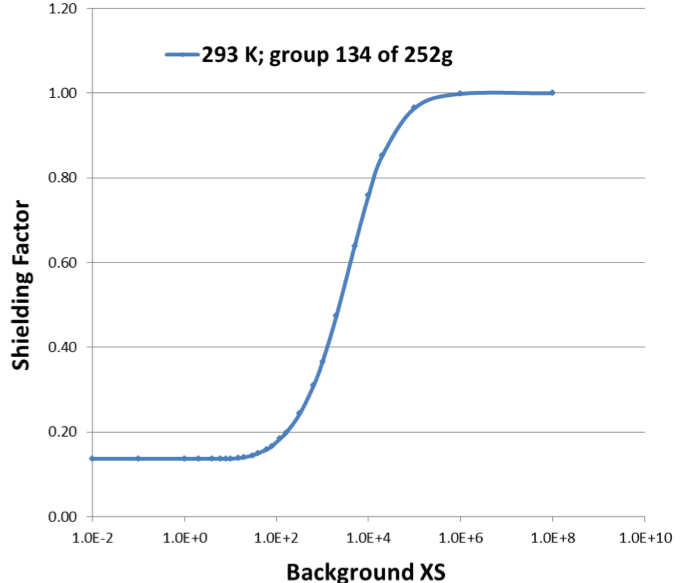
Fig. 7.3.1 Plot of f-factor variation for 238U capture reaction.
Interpolation of the f-factors can be problematic, and several different schemes have been developed for this purpose. Some of the interpolation methods that have been used in other codes are constrained Lagrangian, [BONAMIDYB77] arc-tangent fitting, [BONAMIKid74] and an approach developed by Segev [BONAMISeg81]. All of these were tested and found to be inadequate for use with the SCALE libraries, which may have multiple energy groups within a single resonance. BONAMI uses a unique interpolation method developed by Greene, which is described in [BONAMIGre82]. Greene’s interpolation method is essentially a polynomial approach in which the powers of the polynomial terms can vary within a panel, as shown in Eq. (7.3.25):
where
Fig. 7.3.2 illustrates the expected behavior of Eq. (7.3.22) caused by varying the powers in a panel.
By allowing the power q to vary as a function of independent variable \(sigma\), we can move between the various monotonic curves on the graph in a monotonic fashion. Note that when p crosses the \(p = 1\) curve, the shape changes from concave to convex, or vice versa.
This shape change means that we can use the scheme to introduce an inflection point, which is exactly the situation needed for interpolating f-factors.
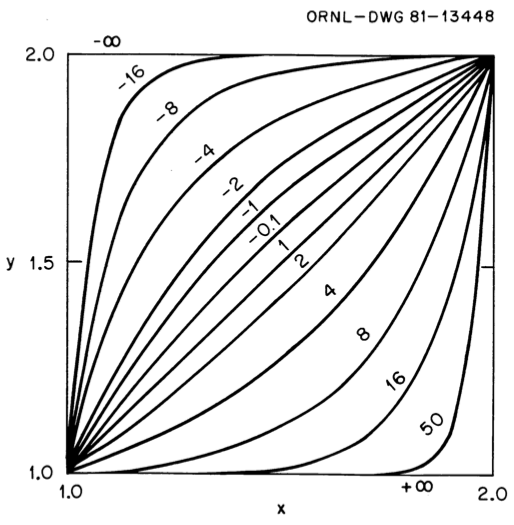
Fig. 7.3.2 Illustration of the effects of varying “powers” in the Greene interpolation method.
Fig. 7.3.3 and Fig. 7.3.3 show typical “fits” of the f-factors using the Greene interpolation scheme for two example cases. Note, in particular, that since this scheme has guaranteed monotonicity, it easily accommodates the end panels that have the smooth asymptotic variation. Even considering the extra task of having to determine the powers for temperature and \(\sigma\)0 interpolations, the method is not significantly more time-consuming than the alternative schemes for most applications.
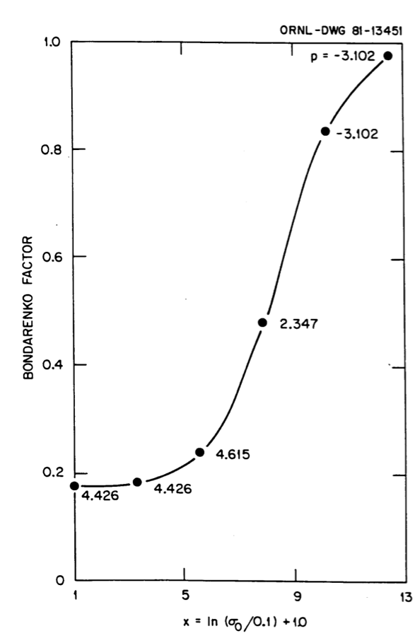
Fig. 7.3.3 Use of Greene’s method to fit the \(\sigma\)0 variation of Bondarenko factors for case 1.
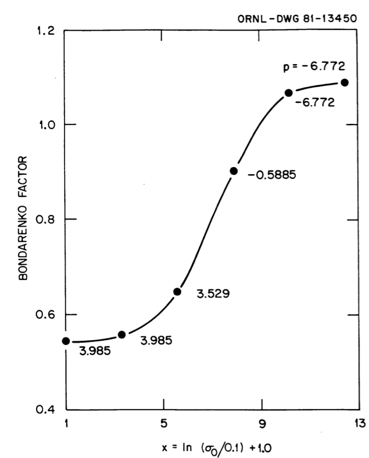
Fig. 7.3.4 Use of Greene’s method to fit the \(\sigma\)0 variation of Bondarenko factors for case 2.
7.3.4. Input Instructions
BONAMI is most commonly used as an integral component of XSProc through SCALE automated analysis sequences. XSProc automatically prepares all the input data for BONAMI and links it with the other self-shielding modules. During a SCALE sequence execution, the data are provided directly to BONAMI in memory through XSProc. Some of the input parameters can be modified in the MOREDATA block in XSProc.
However, the legacy interface to execute stand-alone BONAMI calculations has been preserved for expert users. The legacy input to BONAMI uses the FIDO schemes described in the FIDO chapter of the SCALE manual. The BONAMI input for standalone execution is given below, where the MOREDATA input keywords are marked in bold.
Data Block 1
0$ Logical Unit Assignments [4]
masterlib- input master library (Default = 23)
mwt-not used
msc-not used
newlib-output master library (Default = 22)
1$ Case Description [6]
cellgeometry-geometry description
0 homogeneous
1 slab
2 cylinder
3 sphere
numzones-number of zones or material regions
3. mixlength-mixing table length. This is the total number of entries needed to describe the concentrations of all constituents in all mixtures in the problem.
ib-not used
crossedt-output edit option
0 no output (Default)
1 input echo
2 iteration list, timing
3 background cross section calculation details
4 shielded cross sections, Bondarenko factors
issopt-not used
iropt-resonance approximation option
0 NR (Default) (Bondarenko iterations)
1 IR with potential scattering
2 IR with absorption and potential scattering (Bondarenko iterations)
3 IR with absorption and elastic scattering (Bondarenko iterations)
bellopt-Bell factor calculation option
0 Otter 1 Leslie (Default)
escxsopt-escape cross section calculation option
0 consistent
1 inconsistent (Default)
2* Floating-Point Constants [2]
1. bonamieps-convergence criteria for the Bondarenko iteration (Default = 0.001)
2. bellfact-geometrical escape probability adjustment factor. See notes below on this parameter (Default = 0.0).
T Terminate Data Block 1.
Data Block 2
3$ Mixture numbers in the mixing table [mixlength]
4$ Component (nuclide) identifiers in the mixing table [mixlength]
5* Concentrations (atoms/b-cm) in the mixing table [mixlength]
6$ Mixtures by zone [numzones]
7* Outer radii (cm) by zone [numzones]
8* Temperature (k) by zone [numzones]
9* Escape cross section (cm-1) by zone [numzones]
10$ Not used
11$ Not used
12* Temperature (K) of the nuclide in a one-to-one correspondence with the mixing table arrays.
13* Dancoff factors by zone [numzones]
14* Lbar (\(\bar{\ell }\)) factors by zone [numzones]
T Terminate Data Block 2.
This concludes the input data required by BONAMI.
7.3.4.1. Notes on input
In the 1$ array, cellgeometry specifies the geometry. The geometry information is used in conjunction with the 7* array to calculate mean chord length Lbar if it is not provided by the user in the 14* array.
numzones, the number of zones, may or may not model a real situation. It may, for example, be used to specify numzones independent media to perform a cell calculation in parallel with one or more infinite medium calculations. The geometry description in 1$ array applies only to mean chord length calculations unless it is provided in 14*.
In the 2* array, bonamieps is used to specify the convergence expected on all macroscopic total values by zone, that is, each \({{\Sigma }_{t}}(g,j)\) in group g and zone j is converged so that
The “Bell” factor in the 2* array is the parameter used to adjust the Wigner rational approximation for the escape probability to a more correct value. It has been suggested that if one wishes to use one constant value, the Bell factor should be 1.0 for slabs and 1.35 otherwise. In the ordinary case, BONAMI defaults the Bell factor to zero and uses a prescription by Otter [BONAMIOtt64] to determine a cross-section geometry-dependent value of the Bell factor for isolated absorber bodies. It uses a prescription by Leslie6 to determine the Dancoff factor–dependent values of the Bell factor for lattices, which are much more accurate than the single value. The user who wishes to determine the constant value can, however, use it by inputting a value other than zero.
The 3$, 4$, and 5* arrays are used to specify the concentrations of the constituents of all mixtures in the problem as follows:
Entry 3$ (Mixture Number) 4$ (Nuclide ID) 5* (Concentrations)
1
2
.
.
.
.
mixlength
.
Because of the manner in which BONAMI references the nuclides in a calculation, each nuclide in the problem must have a unique entry in the mixing table. Thus one cannot specify a mixture and subsequently load it into more than one zone, as can be the case with many modules requiring this type of data.
The 12* array is used to allow varying the temperatures by nuclide within a zone. In the event this array is omitted, the 12* array will default by nuclide to the temperature of the zone containing the nuclide.
The mixture numbers in each zone are specified in the 6$ array. Mixture numbers are arbitrary and need only match up with those used in the 3$ array.
The radii in the 7* array are referenced to a zero value at the left boundary of the system.
In the event the temperatures in the 8* array are not bounded by temperature values in the Bondarenko tables, BONAMI will extrapolate using the three temperature points closest to the value. For example, a request for 273 K for a nuclide with Bondarenko sets at 300, 900, and 2,100 K would use the polynomial fit from those three temperature points to extrapolate the 273 K value.
The escape cross sections in the 9* array allow a macro escape cross section (\(\Sigma _{e}^{input}\)) to be specified by zone. (This array can be ignored if Dancoff factors are provided.) If the Dancoff factor for a zone is specified as -1 in the input, then the user-specified escape cross section is used in calculating the background cross sections \(\sigma\)0 as follows:
7.3.5. Sample Problem
In most cases, the input data to BONAMI are simple and obvious because the complicated parameters are determined internally based on the options selected. The user describes his geometry, the materials contained therein, the temperatures, and a few options.
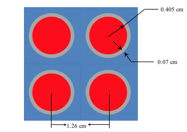
This problem is for a system of iron-clad uranium (U238 – U235 ) fuel pins arranged in a square lattice in a water pool.
Our number densities are
Fuel:
\({{N}_{{}^{235}U}}\) = 1.4987 × 10⁻⁴
\({{N}_{{}^{238}U}}\) = 2.0664× 10⁻²
Clad:
\({{N}_{{}^{56}Fe}}\) = 9.5642× 10⁻⁵
Water:
NH = 6.6662 × 10⁻²
NO = 3.3331 × 10⁻²
For the problem, we choose iropt = 1 (IR approximation with scattering approximated by math:lambda\(\Sigma\) p) and crossedt = 4 for the most detailed output edits. An 8-group test library is used for fast execution and a short output file.
The XSProc/CSAS1X SCALE sequence input file, the corresponding i_bonami FIDO input file created by the sequence under the temporary working directory, and an abbreviated copy of the output from this case follows.
=csas1x
Assembly pin
test-8grp
read comp
' fuel
u-235  1 0 1.4987e-4 297.15 end
u-238  1 0 2.0664e-2 297.15 end
' clad
fe-56  2  0 9.5642e-5 297.15 end
' coolant
h      3 0 6.6662e-2 297.15 end
o      3 0 3.3331e-2 297.15 end
end comp
' ====================================================================
read celldata
latticecell squarepitch  pitch=1.26 3  fuelr=0.405765 1
                                       cladr=0.47498  2 end

moredata iropt=1 crossedt=4 end moredata
end celldata
' ====================================================================
end
FIDO input i_bonami
 -1$$  a0001
     500000
 e
  0$$  a0001
         11           0          18           1
 e
  1$$  a0001
          1           3           5           0           4        1010
          1          -1          -1
 e
 2**  a0001
  1.00000E-03   0.00000E+00
  e
 t
  3$$  a0001
          1           1           2           3           3
 e
  4$$  a0001
      92235       92238       26056        1001        8016
 e
 5**  a0001
  1.49870E-04   2.06640E-02   9.56420E-05   6.66620E-02   3.33310E-02
  e
  6$$  a0001
          1           2           3
 e
 7**  a0001
  4.05765E-01   4.74980E-01   7.10879E-01
  e
 8**  a0001
  2.97150E+02   2.97150E+02   2.97150E+02
  e
 9**  a0001
  1.11870E+00   4.15813E+00   1.78119E-01
  e
 10$$  a0001
      92235       92238       26056        1001        8016
 e
 11$$  a0001
          0           0           0
 e
 13**  a0001
  2.71260E-01   5.20852E-01   9.24912E-01
  e
 14**  a0001
  8.11530E-01   1.38430E-01   4.71798E-01
  e
 15**  a0001
  0.00000E+00   0.00000E+00   0.00000E+00   0.00000E+00
  e
 16$$  a0001
          2           2           2
 e
 17$$  a0001
          0           0           0           0
 e
t
                                   program verification information

                               code system:  SCALE    version:  6.2


          program:  bonami

    creation date:   unknown

          library:  /home02/u2m/Workfolder/sampletmp


        test code:  bonami

          version:  6.2.0

          jobname:  u2m

     machine name:  node22.ornl.gov

date of execution:  04_dec_2013

time of execution:  21:43:54.38
1
                BONAMI CELL PARAMETERS
---------------------------------------------
Bonami Print Option          : 4
BellFactor                   : 0
Bondarenko Iteration eps     : 0.001
Resonance Option             : 1
Bell Factor  Option          : LESLIE
Escape CrossSection  Option  : INCONSISTENT
CellGeometry                 : 2
MasterLibrary                :
Number oF Neutron Groups     : 8
First Thermal Neutron Group  : 5
__________________________________________
Processing Zone               : 1
Mixture Number                : 1
Number Of Nuclides            : 2
Dancoff Factor                : 0.27126
Lbar                          : 0.81153
Escape Cross Section Input    : 1.1187
Material Temeprature          : 297.15

Processing Nuclide :  92235  Number Density : 0.00014987
Processing Nuclide :  92238  Number Density : 0.020664

Bondarenko Iterations
iteration    Nuclide Group   MaxChange   Selfsig0     Effsig0
     1        92235     0             0          0   0
     1        92238     0             0          0   0

Total number of Bondarenko Iterations  : 1
Max Change in Group                    : 0

Group  Eff Macro Sig0      Escape Xsec
   1      0.2351032         0.9075513
   2      0.2351032         0.9075513
   3      0.2351032         0.9075513
   4      0.2351032         0.9075513
   5      0.2351032         0.9075513
   6      0.2351032         0.9075513
   7      0.2351032         0.9075513
   8      0.2351032         0.9075513

---------------------------------------------------
Shielding Nuclide 92235

mt   Group      sig0      infDiluted Xsec    f-factor  shielded Xsec
   1     1    7612.71875         7.19131      0.999998   7.19129
   1     2    7612.71875         10.2521      0.999616   10.2481
   1     3    7612.71875         24.9361       1.00241   24.9963
   1     4    7612.71875         75.1109       1.05902   79.5436
   1     5    7612.71875         56.0286       1.00205   56.1434
   1     6    7612.71875         198.645        1.0008   198.805
   1     7    7612.71875         347.945       1.00024   348.028
   1     8    7612.71875         761.257        1.0066   766.282

mt   Group      sig0      infDiluted Xsec    f-factor  shielded Xsec
   2     1    7612.71875         3.71448      0.999999   3.71448
   2     2    7612.71875         7.63235       0.99935   7.62739
   2     3    7612.71875          11.841      0.999444   11.8345
   2     4    7612.71875         11.5408       1.00561   11.6055
   2     5    7612.71875         12.5449       1.00001   12.545
   2     6    7612.71875         14.2501       1.00007   14.2511
   2     7    7612.71875         14.8125       1.00003   14.8128
   2     8    7612.71875         15.1274       1.00015   15.1297

mt   Group      sig0      infDiluted Xsec    f-factor  shielded Xsec
  18     1    7612.71875         1.21846      0.999996   1.21846
  18     2    7612.71875         1.40834        1.0002   1.40862
  18     3    7612.71875         8.92885       1.00132   8.94062
  18     4    7612.71875         39.2086       1.06274   41.6686
  18     5    7612.71875         32.7026       1.00105   32.737
  18     6    7612.71875         153.511       1.00089   153.647
  18     7    7612.71875         285.775       1.00026   285.848
  18     8    7612.71875         636.445       1.00655   640.611

mt   Group      sig0      infDiluted Xsec    f-factor  shielded Xsec
 102     1    7612.71875        0.060296             1   0.0602962
 102     2    7612.71875        0.317627       1.00352   0.318746
 102     3    7612.71875         4.16593       1.01325   4.22113
 102     4    7612.71875         24.3615       1.07832   26.2695
 102     5    7612.71875          10.781       1.00749   10.8618
 102     6    7612.71875         30.8844       1.00074   30.9073
 102     7    7612.71875         47.3579        1.0002   47.3671
 102     8    7612.71875         109.685       1.00781   110.542

mt   Group      sig0      infDiluted Xsec    f-factor  shielded Xsec
1007     1    7612.71875               0             0   0
1007     2    7612.71875               0             0   0
1007     3    7612.71875               0             0   0
1007     4    7612.71875               0             0   0
1007     5    7612.71875         12.5448       1.00001   12.5449
1007     6    7612.71875         14.2501       1.00007   14.2511
1007     7    7612.71875         14.8125       1.00003   14.8129
1007     8    7612.71875         15.1278       1.00015   15.13

---------------------------------------------------
Shielding Nuclide 92238

mt   Group      sig0      infDiluted Xsec    f-factor  shielded Xsec
   1     1    44.0034676         7.33815      0.999983   7.33803
   1     2    44.0034676         10.3566       1.00418   10.3999
   1     3    44.0034676         15.0517      0.976844   14.7032
   1     4    44.0034676          15.951      0.983793   15.6925
   1     5    44.0034676         9.43867       1.00002   9.43887
   1     6    44.0034676         10.1008       1.00008   10.1015
   1     7    44.0034676         10.7744       1.00004   10.7748
   1     8    44.0034676         12.2124       1.00145   12.2301

mt   Group      sig0      infDiluted Xsec    f-factor  shielded Xsec
   2     1    44.0034676          4.0228      0.999974   4.0227
   2     2    44.0034676         9.05886       1.00575   9.11093
   2     3    44.0034676         14.0213      0.979923   13.7398
   2     4    44.0034676         11.9032       0.98795   11.7598
   2     5    44.0034676         8.86555      0.999984   8.86541
   2     6    44.0034676         9.24452       1.00002   9.24471
   2     7    44.0034676          9.2797       1.00002   9.27987
   2     8    44.0034676          9.3077       1.00009   9.30853

mt   Group      sig0      infDiluted Xsec    f-factor  shielded Xsec
  18     1    44.0034676        0.376356       1.00001   0.376361
  18     2    44.0034676     0.000528746       1.00019   0.000528845
  18     3    44.0034676     0.000308061      0.966052   0.000297603
  18     4    44.0034676     4.75014e-06      0.967842   4.59738e-06
  18     5    44.0034676     2.60878e-06       1.00006   2.60893e-06
  18     6    44.0034676     5.27139e-06       1.00071   5.27512e-06
  18     7    44.0034676      9.3235e-06       1.00018   9.32514e-06
  18     8    44.0034676     1.81868e-05       1.00588   1.82937e-05

mt   Group      sig0      infDiluted Xsec    f-factor  shielded Xsec
 102     1    44.0034676       0.0554327       1.00006   0.0554359
 102     2    44.0034676         0.17972      0.978628   0.175879
 102     3    44.0034676         1.03011      0.934934   0.963087
 102     4    44.0034676         4.04777      0.971568   3.93268
 102     5    44.0034676        0.573119        1.0006   0.573462
 102     6    44.0034676        0.856257       1.00068   0.856839
 102     7    44.0034676         1.49471       1.00017   1.49497
 102     8    44.0034676         2.90465       1.00586   2.92168

mt   Group      sig0      infDiluted Xsec    f-factor  shielded Xsec
1007     1    44.0034676               0             0   0
1007     2    44.0034676               0             0   0
1007     3    44.0034676               0             0   0
1007     4    44.0034676               0             0   0
1007     5    44.0034676         8.86549      0.999984   8.86535
1007     6    44.0034676         9.24445       1.00002   9.24463
1007     7    44.0034676         9.27974       1.00002   9.27992
1007     8    44.0034676         9.30769       1.00009   9.30852
Zone Calculation is completed in 0 seconds
                BONAMI CELL PARAMETERS
---------------------------------------------
Bonami Print Option          : 4
BellFactor                   : 0
Bondarenko Iteration eps     : 0.001
Resonance Option             : 1
Bell Factor  Option          : LESLIE
Escape CrossSection  Option  : INCONSISTENT
CellGeometry                 : 2
MasterLibrary                :
Number oF Neutron Groups     : 8
First Thermal Neutron Group  : 5
__________________________________________
Processing Zone               : 2
Mixture Number                : 2
Number Of Nuclides            : 1
Dancoff Factor                : 0.520852
Lbar                          : 0.13843
Escape Cross Section Input    : 4.15813
Material Temeprature          : 297.15

Processing Nuclide :  26056  Number Density : 9.5642e-05

Bondarenko Iterations
iteration    Nuclide Group   MaxChange   Selfsig0     Effsig0
     1        26056     0             0          0   0

Total number of Bondarenko Iterations  : 1
Max Change in Group                    : 0

Group  Eff Macro Sig0      Escape Xsec
   1     0.0003553244          3.487286
   2     0.0003553244          3.487286
   3     0.0003553244          3.487286
   4     0.0003553244          3.487286
   5     0.0003553244          3.487286
   6     0.0003553244          3.487286
   7     0.0003553244          3.487286
   8     0.0003553244          3.487286

---------------------------------------------------
Shielding Nuclide 26056

mt   Group      sig0      infDiluted Xsec    f-factor  shielded Xsec
   1     1    36461.8672         3.07957       1.00005   3.07972
   1     2    36461.8672         4.68958       1.00091   4.69382
   1     3    36461.8672         7.85712      0.999843   7.85589
   1     4    36461.8672         12.0029             1   12.0029
   1     5    36461.8672         12.3689       1.00001   12.369
   1     6    36461.8672         12.8598       1.00003   12.8602
   1     7    36461.8672         13.5237      0.999906   13.5224
   1     8    36461.8672         15.0714       0.99949   15.0637

mt   Group      sig0      infDiluted Xsec    f-factor  shielded Xsec
   2     1    36461.8672         2.26476       1.00047   2.26583
   2     2    36461.8672          4.6817        1.0009   4.68592
   2     3    36461.8672         7.81457      0.999813   7.81311
   2     4    36461.8672         11.9143             1   11.9143
   2     5    36461.8672         12.0468       1.00001   12.0469
   2     6    36461.8672          12.065       1.00002   12.0653
   2     7    36461.8672         12.0887       1.00005   12.0893
   2     8    36461.8672         12.2042       1.00013   12.2057

mt   Group      sig0      infDiluted Xsec    f-factor  shielded Xsec
 102     1    36461.8672      0.00206393        1.0015   0.00206702
 102     2    36461.8672      0.00787763        1.0035   0.00790524
 102     3    36461.8672       0.0425504       1.00623   0.0428155
 102     4    36461.8672       0.0885525             1   0.0885529
 102     5    36461.8672        0.322101       1.00002   0.322109
 102     6    36461.8672        0.794804        1.0002   0.79496
 102     7    36461.8672         1.43496      0.998734   1.43314
 102     8    36461.8672         2.86723      0.996792   2.85803

mt   Group      sig0      infDiluted Xsec    f-factor  shielded Xsec
1007     1    36461.8672               0             0   0
1007     2    36461.8672               0             0   0
1007     3    36461.8672               0             0   0
1007     4    36461.8672               0             0   0
1007     5    36461.8672         12.0468       1.00001   12.0469
1007     6    36461.8672          12.065       1.00002   12.0653
1007     7    36461.8672         12.0887       1.00005   12.0893
1007     8    36461.8672         12.2042       1.00013   12.2057
Zone Calculation is completed in 0 seconds
BONAMI CELL PARAMETERS
---------------------------------------------
Bonami Print Option          : 4
BellFactor                   : 0
Bondarenko Iteration eps     : 0.001
Resonance Option             : 1
Bell Factor  Option          : LESLIE
Escape CrossSection  Option  : INCONSISTENT
CellGeometry                 : 2
MasterLibrary                :
Number oF Neutron Groups     : 8
First Thermal Neutron Group  : 5
__________________________________________
Processing Zone               : 3
Mixture Number                : 3
Number Of Nuclides            : 2
Dancoff Factor                : 0.924912
Lbar                          : 0.471798
Escape Cross Section Input    : 0.178119
Material Temeprature          : 297.15

Processing Nuclide :   1001  Number Density : 0.066662
Processing Nuclide :   8016  Number Density : 0.033331

Bondarenko Iterations
iteration    Nuclide Group   MaxChange   Selfsig0     Effsig0
     1         1001     0             0          0   0
     1         8016     0             0          0   0

Total number of Bondarenko Iterations  : 1
Max Change in Group                    : 0

Group  Eff Macro Sig0      Escape Xsec
   1       1.494705         0.1593803
   2       1.494705         0.1593803
   3       1.494705         0.1593803
   4       1.494705         0.1593803
   5       1.494705         0.1593803
   6       1.494705         0.1593803
   7       1.494705         0.1593803
   8       1.494705         0.1593803

---------------------------------------------------
Shielding Nuclide 1001

mt   Group      sig0      infDiluted Xsec    f-factor  shielded Xsec
   1     1    4.33502197         2.98905      0.999485   2.98751
   1     2    4.33502197         9.87269      0.999169   9.86448
   1     3    4.33502197         19.9332      0.999972   19.9326
   1     4    4.33502197         20.4672      0.998926   20.4453
   1     5    4.33502197         21.1735       1.00001   21.1736
   1     6    4.33502197         26.1886       0.99995   26.1873
   1     7    4.33502197         35.0621      0.999821   35.0558
   1     8    4.33502197         54.9507      0.997361   54.8057

mt   Group      sig0      infDiluted Xsec    f-factor  shielded Xsec
   2     1    4.33502197         2.98901      0.999485   2.98747
   2     2    4.33502197          9.8726      0.999168   9.86439
   2     3    4.33502197         19.9315      0.999972   19.9309
   2     4    4.33502197         20.4556      0.998926   20.4336
   2     5    4.33502197         21.1321       1.00001   21.1322
   2     6    4.33502197         26.0865       0.99995   26.0852
   2     7    4.33502197         34.8778      0.999829   34.8718
   2     8    4.33502197         54.5786      0.997396   54.4365

mt   Group      sig0      infDiluted Xsec    f-factor  shielded Xsec
 102     1    4.33502197     3.56422e-05       1.00003   3.56433e-05
 102     2    4.33502197     8.96827e-05      0.998165   8.9518e-05
 102     3    4.33502197      0.00171679      0.999794   0.00171643
 102     4    4.33502197       0.0116042       1.00002   0.0116044
 102     5    4.33502197       0.0413709       1.00001   0.0413714
 102     6    4.33502197        0.102043       1.00007   0.10205
 102     7    4.33502197        0.184322      0.998389   0.184025
 102     8    4.33502197        0.372079      0.992163   0.369163

mt   Group      sig0      infDiluted Xsec    f-factor  shielded Xsec
1007     1    4.33502197               0             0   0
1007     2    4.33502197               0             0   0
1007     3    4.33502197               0             0   0
1007     4    4.33502197               0             0   0
1007     5    4.33502197         21.1312       1.00005   21.1322
1007     6    4.33502197         26.0871      0.999927   26.0852
1007     7    4.33502197         34.8779      0.999826   34.8718
1007     8    4.33502197         54.5802      0.997367   54.4365

---------------------------------------------------
Shielding Nuclide 8016

mt   Group      sig0      infDiluted Xsec    f-factor  shielded Xsec
   1     1    45.7377472         2.36081      0.980071   2.31376
   1     2    45.7377472         3.95917      0.995755   3.94236
   1     3    45.7377472         3.84394             1   3.84394
   1     4    45.7377472         3.85289             1   3.85291
   1     5    45.7377472         3.85531       1.00002   3.85537
   1     6    45.7377472          3.8648       1.00006   3.86502
   1     7    45.7377472         3.89139       1.00014   3.89194
   1     8    45.7377472         4.01909       1.00036   4.02056

mt   Group      sig0      infDiluted Xsec    f-factor  shielded Xsec
   2     1    45.7377472         2.34636      0.979939   2.29929
   2     2    45.7377472         3.95907      0.995756   3.94226
   2     3    45.7377472         3.84393             1   3.84393
   2     4    45.7377472         3.85288             1   3.8529
   2     5    45.7377472         3.85529       1.00002   3.85535
   2     6    45.7377472         3.86474       1.00006   3.86496
   2     7    45.7377472         3.89128       1.00014   3.89183
   2     8    45.7377472         4.01888       1.00037   4.02035

mt   Group      sig0      infDiluted Xsec    f-factor  shielded Xsec
 102     1    45.7377472      0.00010111        1.0002   0.00010113
 102     2    45.7377472     0.000101635      0.991292   0.00010075
 102     3    45.7377472     7.10826e-06       1.00036   7.11084e-06
 102     4    45.7377472      7.2788e-06       1.00001   7.27885e-06
 102     5    45.7377472     2.38519e-05       1.00003   2.38526e-05
 102     6    45.7377472     5.83622e-05       1.00019   5.83734e-05
 102     7    45.7377472     0.000105195      0.998729   0.000105061
 102     8    45.7377472     0.000209981      0.996663   0.00020928

mt   Group      sig0      infDiluted Xsec    f-factor  shielded Xsec
1007     1    45.7377472               0             0   0
1007     2    45.7377472               0             0   0
1007     3    45.7377472               0             0   0
1007     4    45.7377472               0             0   0
1007     5    45.7377472         3.85523       1.00003   3.85535
1007     6    45.7377472         3.86483       1.00003   3.86496
1007     7    45.7377472         3.89119       1.00016   3.89183
1007     8    45.7377472         4.01794        1.0006   4.02035
Zone Calculation is completed in 0 seconds
 module: BonamiM  has terminated after a cpu usage of  0.0100  seconds
References
- BONAMIDYB77
W. J. Davis, M. B. Yarbrough, and A. B. Bortz. SPHINX, a one-dimensional diffusion and transport nuclear cross section processing code. Technical Report Westinghouse Advanced Reactors Division report WARD-XS-3045-17, Westinghouse, 8 1977.
- BONAMIGC62(1,2)
Rubin Goldstein and E. Richard Cohen. Theory of resonance absorption of neutrons. Nuclear Science and Engineering, 13(2):132–140, 1962. Publisher: Taylor & Francis.
- BONAMIGre82
N. M. Greene. Method for interpolating in Bondarenko factor tables and other functions. Technical Report, Oak Ridge National Laboratory, Oak Ridge, TN (USA), 1982.
- BONAMIIB64
Igor Ilich Bondarenko. Group constants for nuclear reactor calculations. Consultants Bureau, 1964.
- BONAMIKid74
R. B. Kidman. Improved F-factor interpolation scheme for 1DX. In Transactions of the American Nuclear Society, volume 18. 1974.
- BONAMIKHW21
Kang Seog Kim, Andrew M. Holcomb, and William A. Wieselquist. Spatially Dependent Resonance Self-Shielding Capability for Non-uniform Temperature Profile in SCALE-6.3 XSProc-BONAMI. In M&C 2021. 2021.
- BONAMILam66
John R. Lamarsh. Introduction to nuclear reactor theory. Volume 3. Addison-Wesley Reading, Massachusetts, 1966.
- BONAMILHJ65
D. C. Leslie, J. G. Hill, and A. Jonsson. Improvements to the Theory of Resonance Escape in Heterogeneous Fuel: I. Regular Arrays of Fuel Rods. Nuclear Science and Engineering, 22(1):78–86, 1965. Publisher: Taylor & Francis.
- BONAMIOtt64
John M. Otter. Escape Probability Approximations in Lumped Resonance Absorbers. Technical Report, Atomics International. Div. of North American Aviation, Inc., Canoga Park …, 1964.
- BONAMISeg81
M. Segev. Interpolation of resonance integrals. Nuclear Science and Engineering, 79(1):113–118, 1981. Publisher: Taylor & Francis.
- BONAMIWWCD15
Dorothea Wiarda, Mark L. Williams, Cihangir Celik, and Michael E. Dunn. AMPX: A Modern Cross Section Processing System for Generating Nuclear Data Libraries. Technical Report, Oak Ridge National Laboratory, Charlotte, NC (USA), 9 2015.