6.8. TSURFER: An Adjustment Code to Determine Biases and Uncertainties in Nuclear System Responses by Consolidating Differential Data and Benchmark Integral Experiments
M. L. Williams, B. L. Broadhead, M. A. Jessee, J. J. Wagschal1, and R. A. Lefebvre
ABSTRACT
The TSURFER code uses the generalized linear least-squares method to consolidate a prior set of measured integral responses (such as keff ) and corresponding calculated values obtained using the SCALE nuclear analysis code system. The initial estimates for the computed and measured responses are improved by adjusting the experimental values and the nuclear data used in the transport calculations-taking into account their correlated uncertainties-so that the most self-consistent set of data is obtained. This procedure makes the refined estimates of the calculated and measured responses agree within first-order accuracy, while constraining the data variations to minimize a generalized chi-square parameter. Consolidation of the original integral experiment data and calculated results reduces the prior uncertainty in the response estimates because additional information has been incorporated. The method can also address one or more “application responses” for which no experimental measurements are available. TSURFER computes an updated estimate for the application responses and provides an estimate for the computational bias and application uncertainty. The methodology is useful in validation studies for criticality safety and reactor analysis.
ACKNOWLEDGMENTS
The authors would like to acknowledge R. L. Childs, formerly of ORNL, for his contributions. Development of the TSURFER code was funded by the U.S. Department of Energy Nuclear Criticality Safety Program.
6.8.1. Introduction
This report describes the TSURFER code (Tool for Sensitivity/Uncertainty analysis of Response Functionals using Experimental Results-pronounced “surfer,” with silent “T” like TSUNAMI), which is a functional module in the SCALE sensitivity and uncertainty (S/U) analysis methodology (see the TSUNAMI-1D chapter). The main functions of the code are to (a) compute uncertainties in calculated integral responses such as keff, due to uncertainties in the input nuclear data; (b) reduce discrepancies between the measured and calculated responses by adjusting the nuclear data and experimental values such that the overall consistency is maximized; (c) analyze measured responses from benchmark experiments to establish the bias and associated uncertainty in some application response that has been calculated.
TSURFER utilizes the generalized linear least-squares (GLLS) methodology based on S/U techniques originally developed in the 1970’s and 1980’s for a variety of applications, including nuclear data evaluation, [TSURFER-PRR+74] fast reactor design studies, [TSURFER-PC88, TSURFER-WML+76] and reactor pressure vessel damage predictions [TSURFER-MWB81]. A recent GLLS application has been in the area of criticality safety analysis, in which critical benchmarks are used to validate the computational methodology for predicting subcritical quantities and configurations of fissile materials [TSURFER-BRH+04]. Similar validation procedures also could be performed for other integral responses of interest for nuclear reactor analysis. These include responses such as reactivity coefficients associated with coolant voiding or Doppler broadening, peak power values, or in-core instrumentation readings. Although not limited to this area, the application of TSURFER to criticality safety validation studies is emphasized here.
6.8.1.1. Application to validation studies
Historically the validity of a calculation performed for some application has been established by considering how well the same calculational methods and nuclear data perform for a set of representative benchmark experiments. While a simple comparison of the computed and experimental results is very informative, it does not fully take advantage of the valuable information provided by the measured integral responses. If the original sets of calculated and experimental responses are consolidated in a consistent manner (i.e., correctly accounting for uncertainties), then the “adjusted” results should be a better estimate for the true responses, since the revised response values are based upon more information than was available in either the original calculations or measurements alone. This is essentially a statement of Bayes Theorem from probability theory, which indicates how prior information (calculated responses) can be evolved by incorporating additional information (integral measurements) into more reliable posterior results (the adjusted responses). The equations used for the GLLS methodology are equivalent to those obtained from Bayes Theorem [TSURFER-Hwa88].
Cross-section libraries for neutron transport calculations are processed from fundamental evaluated nuclear data files such as ENDF/B. Because the “true” values of the nuclear data are not known precisely, it is reasonable to view the ENDF data as being selected from a probability distribution of allowable values. Nuclear data uncertainties are described by covariance matrices that contain variances in the group cross sections for a given nuclide and reaction type, as well as covariances arising from correlations between energy groups, and possibly between reactions and materials. Discrepancies in the ENDF nuclear data caused by uncertainties in the evaluation process propagate to errors in group cross sections, which in general cause computed responses to disagree with the corresponding measured values. The GLLS approach considers potential variations in data parameters and measured integral responses that minimize the differences in measured and calculated integral responses (such as keff) for a set of benchmark experiments, taking into account uncertainties and correlations in the ENDF data and in the integral measurements. Since there are generally many more cross-section values than measured integral responses, the determination of the data modifications is an under-determined problem. If the data variations are not performed in a reasonable manner, non-physical changes may be obtained. Data adjustments in the GLLS methodology are constrained by the magnitude of the nuclear data uncertainties and their correlations. TSURFER also accounts for uncertainties and correlations in the integral response measurements, arising from experimental uncertainties in parameters such as enrichment, density, impurities, etc. As long as realistic data covariances are used, the resulting data adjustments may be considered the “best estimates”-within the limitations of the GLLS linearity approximation-for realistic data alterations that improve the computed integral responses. It can be shown that the GLLS equations provide the maximum likelihood estimator for the correct nuclear data if the evaluated nuclear data and system parameters obey a multivariate normal probability distribution [TSURFER-Hwa88].
Some previous studies have applied the GLLS methodology to produce an adjusted nuclear data library in order to improve calculations of nuclear reactors with similar characteristics as the experiments used in the adjustment [TSURFER-TTYS88]. In criticality safety analysis this procedure runs the risk of applying the adjusted library to systems beyond the limits for which the data modifications are appropriate. The usual function of TSURFER is not to output an adjusted nuclear data library but rather to obtain an adjusted application response (keff) and to provide a quantitative estimate for its accuracy. Hence, it is more appropriate to view TSURFER as a tool to establish biases and uncertainties in calculated responses. Nuclear data adjustments are a by-product of this procedure.
Traditional validation of criticality safety calculations estimates the computational bias based on trends in the calculated keff values versus system parameters such as hydrogen-to-fissile ratios (H/X) or energy of average lethargy causing fission (EALF). These trending parameters are frequently used as measures of “similarity” between critical systems, hence their use as bias-predictors. Recent studies have shown that data sensitivity coefficients, either alone or in combination with cross-section uncertainty information, are good indicators of system similarity. Thus S/U-based indices have also been used in trending analyses, analogously to the commonly used physical parameters.5 The input data for S/U trending analysis (i.e., calculated and measured responses, sensitivity coefficients, cross-section and experimental uncertainties) are almost identical to those needed for GLLS analysis; therefore, it is not surprising that some aspects of the TSURFER calculations are also used for trending results. However, TSURFER provides an alternative to the trending approach to determine the bias and can address other validation issues. For example, TSURFER is useful when there are few or no existing experiments that are similar to a particular application area, since the GLLS technique can include individual experiments that separately validate portions of the application area, even though none can be considered entirely similar to the application [TSURFER-Gol04].
6.8.1.2. Types of responses
A response corresponds to a particular integral response type (e.g., keff, reaction rate ratio, material worth, radiation dose, etc.) in a particular nuclear system (e.g., a benchmark experiment or a proposed storage arrangement of reactor fuel assemblies or a reactor core). In the TSURFER input, responses may be classified either as “experiments” or “applications” or “omitted.”
An experiment response has both calculated and measured values input to TSURFER, and these play an active role in the GLLS procedure, which minimizes the difference between the two results. A value for the uncertainty in the measured response and any correlations with other experiments are also input for experimental responses. Examples of experimental integral responses are the multiplication factor for the GODIVA critical benchmark experiment, the measured \(\rho^{28}\) (ratio of epithermal to thermal capture rate for 238U) in the TRX-1 critical benchmark lattice, or the coolant voiding reactivity in a power reactor.
Applications are responses for which a calculated value is known but no measured value is available. Applications often correspond to hypothetical systems being considered within the context of a design study or a criticality safety analysis for which the computational bias and uncertainty are desired. Examples of application responses are the multiplication factor (subcritical) for a proposed fuel assembly storage rack or for a shipping cask. An application response plays a passive role in the GLLS procedure. Since the application has no experimental results, it does not impact the active responses included in the consolidation procedure; conversely, the GLLS procedure may modify the calculated application value if it is “similar” to some of the experimental responses. In this case the application response shares similar data sensitivity characteristics with one or more of the active responses and hence will be indirectly affected by the same data adjustments that impact the similar experimental responses. This provides a systematic, well-defined method for utilizing experimental benchmark measurements to establish a bias and uncertainty in the calculation of application response.
A response designated as omitted in the TSURFER input neither affects other responses nor is affected by them. These responses are completely isolated from the GLLS procedure. This capability is sometimes useful to easily “turn off” an active system to observe its impact on the application results or on the consistency (chi-square) of the set of remaining experimental responses.
6.8.2. Sources of Response Uncertainty
Transport calculations of responses such as the neutron multiplication factor inherently have biases and uncertainties due to several factors that can be grouped into three classes:
numerical approximations in the transport code;
system modeling approximations; and
input data uncertainties.
6.8.2.1. Class-A uncertainties (numerical)
Class-A uncertainties are sometimes referred to as “methods uncertainties.” In Monte Carlo calculations these may be caused by imperfections in random number generation routines, approximations in techniques for scoring neutron multiplication (e.g., incomplete convergence of fission source distribution, neglect of correlations between generations, etc.), and biases from algorithms used to represent nuclear data and to sample probability distributions, as well as the basic statistical uncertainty that is fundamental to the Monte Carlo method. Deterministic methods have uncertainties from using finite space-energy-direction meshes, truncated (rather than infinite) expansions of functions, incomplete convergence of iterations, and especially self-shielding approximations for the multigroup cross sections. Computational benchmark studies often can establish a reasonable upper limit for these effects, which may be judged either as negligible or as requiring some conservative bias to be applied to the application calculations. Here it is assumed that class-A uncertainties in the calculated response can be made acceptably small (e.g., by running more histories or refining mesh sizes) or at least have been previously quantified and can be bounded by a margin applied to the computation. Hence class (A) uncertainties are considered as systematic “tolerance,” and are not addressed in the present GLLS methodology used by TSURFER.
6.8.2.2. Class-B uncertainties (modeling/experimental)
Class-B uncertainties occur because the mathematical model used in the transport computations of an application or an experimental response does not correspond exactly to the “true” system. The response uncertainty caused by modeling effects may be associated with either (i) direct computational simplifications such as omitting or homogenizing some components in the calculation model or (ii) fundamental uncertainties in the material compositions, densities, and dimensions of the experiment. The former are systematic uncertainties similar in effect to Class-A numerical uncertainties and may be addressed in the same manner; that is, by bounding the magnitude of the uncertainty through the applied safety margins. However, the latter are true random uncertainties that in theory have probability distributions, and these may be addressed with the TSURFER code.
Even “clean” critical benchmark experiments have uncertainties in the nominal system parameters-such as fuel enrichment, impurities, densities, critical dimensions, and numerous other components-that may lead to discrepancies in the measured and calculated responses for the system. In TSURFER the impact of these uncertainties is designated as the “experimental uncertainty” in the response, since this uncertainty will be present even if no simplifications or approximations are made in the model used for the transport computation. The terminology is sometimes a source of confusion. For example the measured keff in a critical experiment usually is known to be unity with a very small uncertainty associated with the long, but finite, stable period. While there is little doubt about keff for a critical experiment, there may be considerable uncertainty in the system parameter values describing the benchmark configuration. This contribution to the modeling uncertainty could be justifiably considered either “experimental” (because system parameters such as material compositions and dimensions are specified by the experimentalists) or “computational” (because uncertainties in the system parameters affect the calculation model), but in TSURFER they are designated as experimental uncertainties. In any case the uncertainty in each system parameter must be propagated to an uncertainty in the measured response. For a keff response this may be done experimentally by physically varying the system parameter and measuring the reactivity effect or, more commonly, by performing auxiliary transport calculations to determine the eigenvalue variation. This is discussed in a somewhat more quantitative manner in Sect. 6.8.4.1.
The response uncertainty components associated with the respective modeling uncertainties in system parameters determine the overall experimental uncertainty. Many benchmark experiment descriptions in the International Handbook of Evaluated Criticality Safety Benchmark Experiments [TSURFER-Bri06] include information about uncertainties in the system parameters and their estimated impact on the multiplication factor. The standard deviations in keff due to uncertainties in various system parameters are assigned by the benchmark evaluators based on published or archived experiment descriptions, and sometimes on other considerations.
A complication in specifying experimental uncertainties is how to treat correlations among the experiments. Response correlations in two benchmark experiments may be caused by factors such as use of the same fuel pins and container tank, and common instrumentation (same detectors, hydrometers, etc.). For example, if two different experiments use the same fuel material, then it is not reasonable to conclude that the enrichment in one is too high while the other is too low, even if both differences fall within the specified standard deviation. Reference [TSURFER-WBP01] has shown that these correlations may not be negligible when applying the GLLS technique to a set of benchmark experiments. Only a limited amount of experiment correlation data has been published, but more is expected in future revisions to the International Handbook of Evaluated Criticality Safety Benchmark Experiments. TSURFER allows experimental uncertainties caused by uncertainties in system modeling parameters to be input for individual components and correlation coefficients can be specified for the shared system parameters of each response. This approach provides the capability for users to describe the actual sources of benchmark experiment correlations without having to know the overall correlation between two different experiments. See Sect. 6.8.4.1 and Sect. 6.8.4.2.
6.8.2.3. Class-C uncertainties (nuclear data)
In many applications, the major source of uncertainty in the calculated response is due to uncertainties in evaluated nuclear data such as microscopic cross sections, fission spectra, neutron yield (nu-bar), and scattering distributions that are contained in ENDF/B. These arise from uncertainties in experimental nuclear data measurements, as well as uncertainties in the evaluation process itself, which in general combine differential experimental information with nuclear physics theory to generate the basic data in compilations like ENDF/B. Class-C uncertainties are governed by probability distributions. The actual probabilities are unknown, but the evaluated data values are assumed to represent the mean of the distribution, and the evaluated variance represents a measure of the distribution width. Correlations as well as uncertainties in nuclear data can have a significant impact on the overall uncertainty in the calculated response; thus, it is important to include covariances as well as variances in the TSURFER calculations. The uncertainties in fundamental nuclear data also impact resonance self-shielding of multigroup cross-section values, further contributing to the response uncertainty [TSURFER-WBP01]. In the SCALE S/U methodology the effects of implicit changes in self-shielded cross sections are included in the overall response sensitivity coefficients, rather than in the covariance data, so that the fundamental data uncertainties are isolated from problem-specific effects [TSURFER-LKH+08]
Covariance information is currently quite limited in all evaluated nuclear data compilations such as ENDF/B. A more complete library of multigroup uncertainties has been created for SCALE using data from a variety of sources, including ENDF/B-VI and VII, JENDL3.1, and approximate covariances based on uncertainties in measured integral data and nuclear model calculations [TSURFER-LKH+08, TSURFER-WR08]. A detailed description of the SCALE covariance libraries is found in the COVLIB chapter.
The GLLS methodology in TSURFER is mainly concerned with treating Class-C uncertainties due to nuclear data, along with Class-B experimental uncertainties.
6.8.3. Analysis Procedure
6.8.3.1. Functional relation to other SCALE modules
TSURFER is a functional module within the overall SCALE S/U methodology. Other modules in SCALE and outside SCALE perform complementary calculations and provide data files used by TSURFER, as described below.
PUFF-IV: AMPX code that processes ENDF/B nuclear data covariances and generates multigroup covariance data; creates nuclear data uncertainty files for input to TSURFER.
TSUNAMI-1D/2D/3D SCALE control sequence that computes sensitivity coefficients for keff or other responses in a 1D/2D/3D model of the experiment or application system; creates sensitivity files used by TSURFER.
TSAR: SCALE functional module that computes sensitivity coefficients for eigenvalue-difference responses such as reactor reactivity parameters, using keff sensitivities from a TSUNAMI sequence; creates sensitivity files used by TSURFER.
TSUNAMI-IP SCALE functional module that computes similarity and completeness indices for a set of responses with sensitivity coefficients. Prior to running TSURFER, it may be advantageous to perform scoping studies with TSUNAMI-IP to determine if the selected set of benchmark experiments provides adequate “coverage” for data uncertainties that have a significant impact on the application response.
6.8.3.2. Guidelines for TSURFER analysis
Both active and passive responses may be included in the TSURFER calculation. For example, in criticality safety validation procedures, responses of interest typically correspond to the system multiplication factor, keff. The desired sub-critical design configuration would be a passive application system, while the critical benchmarks used for validation are active experiment systems. TSURFER determines the application bias and uncertainty by propagating data variations obtained from GLLS analysis of the active systems to the calculated multiplication factor of the passive system. The bias represents the change of the application’s original keff as a result of the consolidation of all the active critical benchmark experiments and the adjusted nuclear data parameters. An increase in keff computed for the applications system response indicates that the calculated value was initially too low (a negative bias), and a decrease that the application’s multiplication factor was too high (a positive bias).
TSURFER also computes uncertainties in the initial and adjusted estimates for the system responses (e.g., multiplication factors). These response uncertainties include effects of experimental uncertainties (class-B) and nuclear data uncertainties (class-C) but not the impact of simplifications made to the experiment specifications and numerical approximations (class-A)-which should be included in the safety margin.
Several quantities can be examined to give confidence to the predicted results [TSURFER-BHCP99, TSURFER-BHP99]. The first is the completeness parameter, R, given in the output of the TSUNAMI-IP code. It has been suggested that values of R greater than about 0.7-0.8 for a set of active experiments indicate adequate cross-section coverage for an application response in the GLLS procedure; however, this is a preliminary conclusion that may change as more experience is gained [TSURFER-Gol04].
The chi-square (\(\chi^2\)) statistic indicates the overall consistency of the suite of benchmarks and is key to proper interpretation of the TSURFER results. The value of \(\chi^2\) per degree of freedom represents the average discrepancy between the calculated and measured responses, expressed in units of the combined variance of the calculation plus experiment. Values of chi-square per degree of freedom ideally should be within about \(\pm\)20% of unity, indicating that the calculations and measurements on average agree within about one standard deviation. Results in which this test is not strictly met may still be valid, but in general these should be viewed with skepticism unless the reasons for the test failure are understood. An excessively large \(\chi^2\) can lead to unreliable results in the GLLS adjustment. TSURFER provides the total \(\chi^2\) value, as well as estimated contributions from each experiment (see Sect. 6.8.4.2.1). Individual \(\chi\)2 values suggest which experiments may contain inconsistencies (i.e., the difference between the measured and calculated keff is larger than their combined uncertainties).
Several methods can be used to improve the initial value of chi-square. One approach is to reevaluate the measurement uncertainties and their correlations for identified discrepant experiments. If the experimental or data uncertainties are underestimated, the data adjustments will correspond to an excessive number of standard deviations, as reflected in high \(\chi\)2 values. Values of \(\chi\)2 that are too low suggest that the input uncertainty estimates may be too high, and again a reevaluation should be considered. Thus it is quite important to utilize realistic (not conservative) estimates for the uncertainties in nuclear data and experimental measurements.
Even when best estimates are used for all input uncertainties, it is not uncommon to encounter a few active responses that are inconsistent with the others, especially when dealing with a large number of benchmark experiments. In this case the best alternative to improve \(\chi^2\) is to remove the outliers, either by transforming those experiments into passive responses or by omitting them entirely from the GLLS adjustment. TSURFER provides a “chi-square filtering” procedure that automatically omits inconsistent experiments until a specified target value of chi-square is achieved. Several options are provided to select the experiments to be omitted, as discussed in Sect. 6.8.4.2.1. Omitted experiments should be examined to ensure that simple errors in the problem description are not present.
An internal consistency test such as described in [TSURFER-BHCP99] also may be useful. The consistency test is performed by changing one of the benchmark experiments that is similar (see Sect. 6.8.4.3) to the application response into a passive, pseudo-application response. The predicted bias for this passive response should be close to that of the original application; furthermore, in this case the bias prediction can be checked because this passive response actually has a measured experimental value.
6.8.3.3. Required data for TSURFER
Active and passive responses considered in the GLLS analysis should have sensitivity data provided for each nuclide-reaction pair that significantly impacts the response. The sensitivity coefficients are pre-calculated using other SCALE modules as described in Sect. 6.8.3.1 and are stored in individual files for each response included in the TSURFER analysis. The sensitivity data files must be in one of the SCALE sensitivity data formats described in Data File Formats. The locations of the sensitivity files are specified in the TSURFER input data. It is not required for all sensitivity files to have the same group structures; for example, the sensitivity coefficients for one response may have been computed using a 238-group cross-section library, while sensitivities for another response could have a 44-group structure. Whatever the group structure of the sensitivity data, it is mapped into the same group structure as the covariance file. At present the SCALE covariance files use the SCALE 56-group structure by default.
A file of nuclear data covariances also must be input to the TSURFER calculation. The covariance data file must be in COVERX format described in the COVERX format section. SCALE includes a comprehensive applications-oriented covariance library that includes evaluated covariances taken from ENDF/B-VII, ENDF/B-VI, and JENDL nuclear data files [TSURFER-WR08] described in the COVLIB chapter. Ideally, the covariance files should contain data for all nuclide-reaction pairs on the response sensitivity data files. However, cross-section covariance data are not available for all nuclide-reaction pairs. Nuclide-reaction pairs without available covariance data are omitted from the GLLS analysis, but it is assumed that either the cross-section covariance data values for these pairs are well known (i.e., small uncertainties) or that the sensitivity to these nuclide-reaction pairs is small. Where these assumptions hold, the cross sections for these nuclide-reaction pairs should not be adjusted and can be omitted from the GLLS analysis. For situations where these assumptions are judged to be invalid, the use of GLLS analysis is not appropriate. However, TSURFER provides several input options to define uncertainty values for nuclide-reaction pairs with missing covariance data to assess the impact of the additional covariance data on the GLLS analysis. These input options are discussed in more detail in Sect. 6.8.5.1 and Sect. 6.8.5.3.
6.8.4. TSURFER Computation Methodology
A recent detailed derivation of the GLLS formalism is given in [TSURFER-BHCP99]. The general formalism allows cross correlations between the initial integral experiment measurements and the original nuclear data, such as would be present if the calculations used a previously “adjusted” library of nuclear data. Since this is not normally done in SCALE, correlations between the benchmark experiment measurements and the cross-section data in the multigroup libraries are not considered in the TSURFER code; therefore, the GLLS equations presented here are somewhat simplified compared to the more general expressions in [TSURFER-Wil86].
At present, the SCALE cross-section-covariance data files characterize nuclear data uncertainties in terms of relative covariances. Therefore, response sensitivity data in TSURFER are defined in terms of relative changes in the nuclear data. An absolute response sensitivity is defined as an absolute change in response due to a relative change in the nuclear data, that is,
In this equation, R represents the response, \(\alpha\) represents the nuclear data, and the tilde will be used to represent absolute sensitivity and uncertainty data. Likewise, a relative response sensitivity is defined as a relative change in response due to a relative change in the nuclear data, that is,
The initial development that follows is for relative, rather than absolute, response sensitivity and uncertainty parameters. It is then shown how to express the quantities in absolute form for reactivity analysis and mixed relative-absolute form for combined keff and reactivity analysis. A summary of the notation and definitions used in this section can be found in TSURFER Appendix A: Sensitivity/Uncertainty Notation.
The methodology consists of calculating values for a set of I integral responses (keff, reaction rates, etc.), some of which have been measured in selected benchmark experiments. Responses with no measured values are the selected “applications,” described previously. The set of measured response values {mi ; i=1,2,…., I} can be arranged into an I-dimension column vector designated as m. By convention the (unknown) experimental values corresponding to applications are represented by the corresponding calculated values. As discussed in Sect. 6.8.2.2, the measured integral responses have uncertainties—possibly correlated—due to uncertainties in the system parameter specifications. The I \(\times\) I covariance matrix describing the relative experimental uncertainties is defined to be C\(_{\bf{mm}}\).
The calculated integral values for each experiment and application are obtained by neutron transport calculations, producing a set of calculated responses {ki ; i=1,2,…., I} arranged in a I-dimension vector k. The multigroup cross-section data for all nuclide-reaction pairs used in the transport calculations of all responses comprise a set {\(\alpha\)n ; n=1,2,…., M}, where M is the number of unique nuclide-reaction pairs multiplied by the number of energy groups. It is convenient to arrange these data into a M-dimensional column vector \(\mathbf{\alpha}\), so that the dependence of the initial calculated responses upon the input nuclear data values can be indicated as k = k(\(\alpha\)). The prior covariance matrix for the nuclear data is equal to the M \(\times\) M matrix \(\mathbf{C}_{\mathbf{\alpha \alpha }}\), which contains relative variances along the diagonal and relative covariances in the off-diagonal positions. These data describe uncertainties in the infinitely dilute multigroup cross sections.
Nuclear data uncertainties cause uncertainties in the calculated response values. In general, these uncertainties are correlated because the same nuclear data library is used for all the transport calculations. The covariance matrix describing uncertainties in the calculated responses due to class-C uncertainties is designated as C\(_{\mathbf{kk}}\). Using expressions for propagation of error (the so called sandwich rule), the following relationship is obtained for the relative uncertainty in the calculated responses:
where \(\mathbf{S}_{\mathbf{k} \boldsymbol{\alpha}}\) is the relative sensitivity matrix, whose (i, n) element is equal to the relative sensitivity of the ith response with respect to the nth data value, that is, \(\frac{1}{\mathrm{R}_{\mathrm{i}}} \frac{\partial \mathrm{R}_{\mathrm{i}}}{\partial \alpha_{\mathrm{n}}} \alpha_{\mathrm{n}}\). Sensitivity coefficients appearing in the sensitivity matrix are computed using first-order perturbation theory. A description of the equations used to compute sensitivity coefficients using first order perturbation theory can be found in [TSURFER-Wil86] or in the SAMS chapter. In the SCALE methodology, the sensitivity coefficients consist of an “explicit” component that accounts for the direct impact of the data on the neutron transport calculation, as well as an “implicit” component that accounts for its impact on other self-shielded multigroup data [TSURFER-WBP01]. For example, a variation in the hydrogen multigroup elastic cross section has an explicit effect on keff through its impact on neutron moderation and leakage in the transport solution and has an implicit effect on the self-shielded 238U multigroup cross sections, which causes additional change in keff. Because self-shielding effects are addressed through the sensitivity coefficients, the nuclear data uncertainties in the covariance matrix correspond to the infinitely dilute values.
Each row i of the sensitivity matrix contains sensitivity coefficients for all nuclear data used in the transport calculation of response i. These data also can be arranged into an M-component sensitivity vector Si for a particular response “i”, which may be either an experiment or application. For example, the sensitivity vector Si is an M dimensional vector whose nth element is equal to the sensitivity coefficient of response “i” to data element \(\alpha_n\) as specified previously.
It is often convenient to express covariance matrices in terms of standard deviations [represented as \(\sigma\)i for variable i] and correlation coefficients [represented by \(\rho_{i,j}\) for the variable pair (i,j)]. The correlation coefficient is related to the corresponding covariance value by the equation
Correlation coefficients, which have values between -1 and 1, indicate the degree of correlation between the pair of variables, where a value of 1.0 indicates full correlation, 0.0 no correlation, and -1.0 full anti-correlation. Using matrix notation, relative standard deviations are arranged in a diagonal matrix \(\boldsymbol{\sigma}\) and the correlation coefficients in a square matrix R (symmetrical, but generally non-diagonal). The previously defined covariance matrices can be expressed as follows:
Eq. (6.6.3) and Eq. (6.8.7) can be substituted into Eq. (6.8.3) and rearranged to relate the nuclear data correlations to the correlations in the computed responses:
The bracketed term on the right side of the above equation is an I \(\times\) M matrix whose elements equal the number of relative standard deviations (\(\boldsymbol{\sigma}_{\mathbf{k}}\)) that the response changes, due to a one relative standard deviation change in the nuclear data (\(\boldsymbol{\sigma}_{\boldsymbol{\alpha}}\)). Even if the nuclear data are not correlated—that is, \(\mathbf{R}_{\boldsymbol{\alpha}\boldsymbol{\alpha}}\) is an identity matrix—\(\mathbf{R}_{\mathbf{kk}}\) is generally not diagonal.
The expressions thus far describe relative response sensitivities and covariances (i.e., uncertainties). Similar expressions can also be derived for absolute quantities. In this report, absolute response sensitivities and covariances are denoted by a tilde, such as \({{\mathbf{\tilde{C}}}_{\mathbf{mm}}}\), \(\,{{\mathbf{\tilde{C}}}_{\mathbf{kk}}}\), and \(\mathbf{\tilde{S}}_{\mathbf{k} \boldsymbol{\alpha}}\), which are explicitly defined in Appendix A.
TSURFER allows for a mixed relative and absolute response sensitivities and covariances to be used in the analysis. In the TSURFER input (described in Sect. 6.8.5), each response is designated as an absolute-formatted response or a relative-formatted response using the input keywords “absolute” or “relative”. This flexibility allows for the simultaneous use of both relative-formatted keff sensitivity data (generated by TSUNAMI modules) and absolute-formatted eigenvalue-difference sensitivity data (generated by TSAR) in the same analysis. In this report, mixed relative-absolute response sensitivities and covariances are denoted by a caret, such as \({{\mathbf{\hat{C}}}_{\mathbf{mm}}}\), \(\,{{\mathbf{\hat{C}}}_{\mathbf{kk}}}\), and \(\mathbf{\hat{S}}_{\mathbf{k} \boldsymbol{\alpha}}\).
6.8.4.1. Representation of experimental uncertainty components
Experimental uncertainties (i.e., type-B uncertainties as described in Sect. 6.8.2.2) may be entered directly in the TSURFER input, or alternatively, it may be specified by defining individual “uncertainty components.” The latter approach is useful in defining experimental correlations between measured responses. In this case, an index ” \(\ell\) ” is introduced to identify the response uncertainty components associated with a particular system parameter, p\(_{\ell}\). For example, the measured keff uncertainty components for a particular critical experiment consisting of uranyl nitrate dissolved in water might correspond to the following eight p\(_{\ell}\) contributors, as identified by the value of (\(\ell\)): (1) isotopic composition; (2) fuel concentration in the solution; (3) solution density; (4) excess acid concentration in the solution; (5) fuel impurities; (6) dimension of the solution tank; (7) thickness of the solution tank; (8) composition of the tank [TSURFER-Bri06].
The relative standard deviation of a measured response mi due to an uncertainty in the system parameter p\(_{\ell}\) is designated as the uncertainty component \(\sigma _{m,i}^{\left( \ell \right)}\). Assuming that uncertainties in system parameters are uncorrelated, the response uncertainty component is related to the uncertainty in system parameter p\(_{\ell}\) by the expression
where \({{\sigma }_{{{p}_{\ell }}}}\) is the relative standard deviation of system parameter p:\(_{\ell}\) and \(\text{S}_{{{\text{m}}_{\text{i}}}{{\text{p}}_{\ell }}}^{{}}\) is the relative sensitivity coefficient relating p\(_{\ell}\) to the measured response mi. In principle, the system parameter values and uncertainties could be treated directly in the TSURFER calculation by providing the sensitivity coefficients \(\text{S}_{{{\text{m}}_{\text{i}}}{{\text{p}}_{\ell }}}^{{}}\), thus allowing the experiment parameters to be included in the GLLS adjustment. However, at the present time the response uncertainty components \(\boldsymbol{\sigma}_{m, i}^{(\ell)}\) must be determined prior to the TSURFER calculation and are read into TSURFER. Values for the response uncertainty components sometimes can be found in the benchmark experiment specifications [TSURFER-Gol04], or auxiliary sensitivity analysis may be necessary. The relative experimental standard deviation of the ith measured response is calculated from
The (i,i) diagonal element of the relative covariance matrix corresponds to the relative experimental variance in response i, which is equal the square of \(\sigma _{m,i}^{{}}\) above. Note that similar expressions can be derived for uncertainty components using absolute sensitivities and uncertainties. For absolute-formatted responses, the uncertainty components on the TSURFER input must be entered in terms of absolute standard deviation. This is discussed in more detail in Sect. 6.8.5.2.
If a different response j is measured in a benchmark system that shares some or all of the same uncertainty components as response i, then the two experiment responses have correlated uncertainties. In such a case the (i, j) element of the relative covariance matrix \({{\mathbf{C}}_{\mathbf{mm}}}\) is equal to
and the total correlation coefficient for response pair (i, j) is
where \(\rho _{\text{i,j}}^{(\ell )}\). is the correlation coefficient for responses i and j due uncertainty component \(\ell\).
TSURFER allows the user to input text-identifiers for the various experiment uncertainty components, along with the associated values for relative standard deviations, \(\sigma _{\text{m,i}}^{\text{(}\ell \text{)}}\). Response correlation coefficients \(\rho _{\text{i,j}}^{(\ell )}\) can be input for each type of uncertainty component, by response pair (i, j).
The previous discussion applies only to experiment responses for which measurements have been performed. In the case of an application response for which no experimental measurement is known, the uncertainty is set internally by TSURFER to the large value of 1010, to approximate the “infinite” uncertainty in the unknown measurement, and correlations to other responses are set to zero. The large uncertainty for an application response has the effect of letting the response “float” in a passive manner; that is, the application response has a negligible effect on the adjustment of active responses, but the GLLS consolidation of the active responses with finite uncertainties can impact the adjusted value for the application.
6.8.4.2. Generalized linear least-squares equations
Discrepancies in the calculated and measured responses are defined by the I dimensional column vector
In TSURFER the components of d corresponding to application responses are set to zero because applications have no measured values. Using the standard formula for propagation of error and assuming no correlations between k and m, the relative uncertainty matrix for the discrepancy vector d can be expressed as the I by I matrix:
where the expression in Eq. (6.8.3) was substituted for C\(_{\mathbf{kk}}\), and F\(_{\mathbf{m}/ \mathbf{k}}\) is an I \(\times\) I diagonal matrix containing m/k factors, that is, \(\frac{E}{C}\) factors (ratio of experimental to calculated response values). The inverse of the matrix C\(_{\mathbf{dd}}\) appears in several expressions presented later in this section. In TSURFER the inversion is performed using routines from the LINPACK software package.
The goal of the GLLS method is to vary the nuclear data \(\left(\alpha \rightarrow \alpha^{\prime}\right)\) and the measured integral responses \(\left(\mathrm{m} \rightarrow \mathrm{m}^{\prime}\right)\), such that they are most consistent with their respective uncertainty matrices, \(\mathbf{C}_{{\mathbf{\alpha \alpha }}}\) and C\(_{\bf{mm}}\). This is done by minimizing chi-square, expressed as
where \(\Delta \alpha_{i}=\frac{\alpha_{i}^{\prime}-\alpha_{i}}{\alpha_{i}}\) and \(\Delta \mathrm{m}_{i}=\frac{\mathrm{m}_{i}^{\prime}-\mathrm{m}_{i}}{\mathrm{~m}_{i}}\). Eq. (6.8.15) is rearranged to give
Eq. (6.8.16) expresses the variations in the nuclear data and measured responses in units of their respective standard deviations; that is, \(\mathbf{\left[\boldsymbol{\sigma}_{\boldsymbol{\alpha}}^{-1} \Delta \boldsymbol{\alpha}\right]}\) and \(\left[\boldsymbol{\sigma}_{\mathbf{m}}^{-1} \boldsymbol{\Delta} \mathbf{m}\right]\)
Chi-square is a quadratic form indicating the squared magnitude of the combined data variations with respect to their uncertainties. This is easily seen for the simple case in which \(\mathbf{R}_{{\mathbf{\alpha \alpha }}}\)-1 and R\(_{\bf{mm}}\)-1 in Eq. (6.8.16) are identity matrices, so that Eq. (6.8.16) reduces to just the diagonal contributions:
The first term on the on the right side of Eq. (6.8.17) is equal to the sum of the squares of the individual nuclear data variations expressed in units of their standard deviations while the second term represents a similar quantity for the measured integral responses. In the general case where correlations exist, the inverse matrices in Eq. (6.8.16) are not diagonal, and the value of chi-square must be evaluated using the indicated matrix multiplication.
Thus it can be seen that the GLLS method determines adjustments in the nuclear data and experimental measurements that (a) make the calculated and measured responses agree [i.e., \(k^{\prime}=k^{\prime} \left(\alpha^{\prime}\right) = m^{\prime}\) within the limitations of first-order sensitivity theory], and (b) minimize Eq. (6.8.15) so that the adjustments are most consistent with the data uncertainties. Although many possible combinations of data variations may make \(k^{\prime}=m^{\prime}\), there is a unique set that also minimizes \(\chi^2\).
Note
In TSURFER the term “chi-square” normally is meant to signify the minimum value of the quadratic form in Eq. (6.8.15). The significance of this minimum value is discussed in Sect. 6.8.4.2.1.
The following variations minimize Eq. (6.8.15), subject to the constraint \(k^{\prime} \left(\alpha^{\prime}\right) = m^{\prime}\) [TSURFER-Wil86] and the linearity condition \([\boldsymbol{\Delta} \mathbf{k}]=\mathbf{S}_{\mathbf{k} \boldsymbol{\alpha}}[\mathbf{\Delta} \boldsymbol{\alpha}]\) where \(\Delta \mathrm{k}_{i}=\frac{\mathrm{k}_{i}^{\prime}-\mathrm{k}_{i}}{\mathrm{k}_{i}}\):
In the above equations the initial response discrepancy vector d is operated on by the transformation matrix in square brackets to obtain the desired variations in nuclear data and integral measurements; thus, it is the discrepancy components that drive the adjustments. If the linearity assumption is valid, then the changes in the calculated responses are found to be
Eq. (6.8.20) relates the adjustments in calculated responses, measured responses, and nuclear data.
As previously discussed, consolidation of the calculated and measured responses reduces the prior uncertainties for \(\alpha^{\prime}\), m, and k because additional knowledge has been incorporated. This is indicated by their modified covariance matrices \(\mathbf{C}_{\boldsymbol{\alpha}^{\prime} \boldsymbol{\alpha}^{\prime}}\), \(\mathbf{C}_{\mathbf{m}^{\prime} \mathbf{m}^{\prime}}\), \(\mathbf{C}_{\mathbf{k}^{\prime} \mathbf{k}^{\prime}}\), respectively, given by [TSURFER-Wil86]
If all the responses on the TSURFER input are relative formatted, then the adjusted data and response values edited by TSURFER are obtained from Eq. (6.8.18)-Eq. (6.8.20), while the square roots of diagonal elements in Eq. (6.8.21)-Eq. (6.8.23) correspond to the edited values for adjusted uncertainties in the nuclear data and in the experiment responses, respectively.
The adjustment formulas must be modified slightly to be consistent with the absolute-formatted responses. In the following expressions, absolute response covariance and response sensitivity data are denoted by a tilde [see Appendix A.]:
Relative covariances for the posterior values of the nuclear data and measured responses are given as
If all the responses on the TSURFER input are absolute formatted, the adjusted data and response values edited by TSURFER are obtained from Eq. (6.8.26)-Eq. (6.8.28), while the square roots of diagonal elements in Eq. (6.8.29)-Eq. (6.8.30) correspond to the edited values for adjusted uncertainties in the nuclear data and in the experiment responses, respectively.
The adjustment formulas again must be modified slightly given a set of mixed relative/absolute-formatted responses. In the following expressions, mixed response covariance and response sensitivity data are denoted by a caret (see Appendix A.), and \({{\mathbf{\hat{F}}}_{\mathbf{m/k}}}\) is an I \(\times\) I diagonal matrix containing m/k factors for relative-formatted responses or a value of one for absolute-formatted responses:
Covariances for the posterior values of the nuclear data and measured responses are given as
If responses on the TSURFER input are both relative formatted and absolute formatted, the adjusted data and response values edited by TSURFER are obtained from Eqs. Eq. (6.8.35)-Eq. (6.8.37), while the square roots of diagonal elements in Eqs. Eq. (6.8.38)-Eq. (6.8.39) correspond to the edited values for adjusted uncertainties in the nuclear data and in the experiment responses, respectively.
6.8.4.2.1. Consistency relations and chi-square filtering
The variations for \(\Delta m\) and \({\Delta}{\alpha}\) defined by Eq. Eq. (6.8.18) and Eq. Eq. (6.8.19) are those that give the smallest value of the quadratic form \(\chi\)2. This minimum \(\chi\)2 value is found by substituting these equations into Eq. Eq. (6.8.15):
It is interesting to observe that Eq. Eq. (6.8.40) does not depend upon adjustments in nuclear data or integral experiments and physically expresses a measure of the initial discrepancies (d) in all responses, compared to their combined calculation and experiment uncertainties (\(\mathbf{C}_{\mathbf{k k}}+\mathbf{F}_{\mathbf{m} / \mathbf{k}} \mathbf{C}_{\mathbf{m} \mathbf{m}} \mathbf{F}_{\mathbf{m} / \mathbf{k}}\)). In fact, the parameter is identical to the chi-square statistic discussed in Sect. 6.8.3.2 that denotes consistency between the calculations and measurements. Equation Eq. (6.8.40) can be viewed as an inherent limit on the consistency of the GLLS adjustment procedure. If the initial calculated and measured responses are not consistent with their stated uncertainties, then adjustments in nuclear data and experiment values obtained by TSURFER cannot be consistent either.
TSURFER provides an option for “chi-square filtering” to ensure that a given set of benchmark experiments is consistent; that is, that the input responses have an acceptable \(\chi _{\min }^{2}\) defined by Eq. (6.8.40). The code progressively removes individual experiments until the calculated \(\chi _{\min}^{2}\) is less than the input target value “target_chi”. Each iteration removes one experiment estimated to have the greatest impact on chi-square per degree of freedom. The method used to assess individual contributions to \(\chi_{\min }^{2}\) is specified by input parameter “chi_sq_filter”, which refers to the different approaches described below.
Independent Chi-Square Option (chi_sq_filter=independent).
The consistency of the i-th measured and calculated response values, disregarding any other integral response, is equal to the discrepancy in the measured and calculated value squared divided by the variance of the discrepancy of the i-th response:
Equation Eq. (6.8.41) is strictly valid only when no correlations exist, but it may be a useful approximation to estimate the experiment having the greatest impact on chi-square per degree of freedom. Hence, this expression is called the “independent chi-square” approximation in TSURFER. This approximation executes fast since no matrix inversions are required.
Diagonal Chi-Square Option (chi_sq_filter=diagonal)
The “diagonal chi-square” approach uses diagonal values of the original inverse \(\mathbf{C}_{\mathbf{dd}}\) matrix to estimate the experiment having the greatest impact on chi-square per degree of freedom:
In this method the correlations in all responses are taken into account to some extent. The original \(\mathbf{C}_{\mathbf{dd}}^{-1}\). is used in each iteration; therefore, the diagonal chi-square method requires only a single matrix inversion.
Iterative-Diagonal Chi-Square Option (chi_sq_filter=iter_diag).
This approach is identical to the diagonal chi-square method, except that an updated value of is computed each iteration to re-evaluate the total chi-square from Eq. Eq. (6.8.40). Thus one matrix inversion is performed per iteration.
Delta Chi-Square Option (chi_sq_filter=delta_chi).
The most rigorous method to determine the impact of an individual response on the overall consistency is called the “delta chi-square” method in TSURFER. This method [TSURFER-YWMW80] calculates the change in chi-square whenever a particular response is omitted for the analysis; that is, omitting the ith response results in
where \(\mathbf{d}_{\neq i}\) and \(\mathbf{C}_{\mathbf{d d}}^{\neq \mathrm{i}}\) are, respectively, the discrepancy vector and discrepancy covariance with response i omitted. While Eq. Eq. (6.8.43) is the most rigorous method, it also requires the most computation effort. A matrix inversion must be performed for every omitted response, in each iteration. For SCALE 6.3, the runtime of this method was reduced by using the matrix inversion lemma to compute the inverse of each submatrix, according to the method of [TSURFER-JRCMPR16].
It has been observed that independent chi-square and diagonal chi-square options execute fast but often eliminate more experiments than necessary to obtain the target chi-square value. The diagonal chi-square option is somewhat faster than the iterative-diagonal chi-square option but also sometimes omits more than the minimum number of experiments. The delta chi-square option is currently default in TSURFER.
6.8.4.2.2. Expressions for computational bias
The computational “bias” is defined here as the observed difference between a calculated and measured response. In conventional validation studies the expected bias in an application response (for which there is no measurement, by definition) often is estimated as the sample mean of the biases for a set of benchmark experiments and the uncertainty in the application bias is estimated by the sample standard deviation of the experimental biases.
The GLLS technique provides another method to compute the bias of an application response. The application response bias \(\beta_a\) is defined as the expected deviation of the original calculated response ka from the best estimate of the measured response, which is unknown but has some probability distribution. Note that if the application response actually did have a prior measured value ma, then the best estimate for the experiment value would be the final adjusted value ma’ obtained from the GLLS procedure. For this reason the notation ma’ is used here to represent the (unknown) best estimate for the application’s projected measured response, so that
where E is the expectation operator. The application’s projected experiment value can be expressed as \(m_a^{\prime} = k_a \left( \alpha^{\prime} \right) - \delta m_a\), where \(\delta m_a\) represents the difference between the best computed response obtained with the adjusted data \(\alpha^{\prime}\) and the expected value of the experimental measurement. Therefore Eq. Eq. (6.8.44) can be expressed
Recall that all experiment responses are sure to have \(\delta m_i = 0\), because the GLLS procedure forces k’=m’ within the approximation of first-order theory. However, \(\delta m_a \left(= k_a^{\prime} - m_a^{\prime} \right)\) for the application is not guaranteed to be zero, since there is no known measured value. Nevertheless the application response calculated using the best cross sections \(\alpha^{\prime}\) should approach the desired (unknown) experiment value if a “sufficient” number of experiments similar to the application of interest are considered [TSURFER-BHCP99] so that under these conditions \(E\left[ \delta m_a \right] \rightarrow 0\) for the application as well. More details concerning the suitable degree of similarity and the sufficient number of experiments necessary for convergence of the GLLS methodology are discussed in other publications [TSURFER-BHCP99, TSURFER-BHP99, TSURFER-MWB81, TSURFER-PC88]. TSURFER also provides an automated procedure to examine the convergence of the bias, which is described in Sect. 6.8.4.4.
Assuming an adequate benchmark data base such that \(E\left[ \delta m_a \right] \rightarrow 0\), Eq. Eq. (6.8.45) simplifies to
or, stated in absolute terms,
In the above equations \(\mathbf{S_a}\) is the column vector of relative sensitivities for the application response. A negative bias indicates that the original computed value was too low; therefore, the adjusted application result will be higher than the original (\(k_a^{\prime} > k_a\)). Similarly, a positive bias means that the original response was calculated too high, and therefore \(k_a^{\prime} < k_a\).
6.8.4.3. Expressions for response similarity parameters
TSURFER estimates the similarity in a pair of responses using one of three internally computed similarity coefficients-respectively designated as E, G, and C-specified by the input parameter “sim_type”. These are essentially equivalent to the corresponding similarity coefficients described in [TSURFER-BRH+04], although there are slight differences in the definitions of E and G. Similarity coefficients are defined so that a value of zero indicates no similarity between the systems, and unity is maximum similarity. It is also theoretically possible, but unusual, to have a negative similarity in the range [-1,0], indicating systems that are “anti-correlated” in some sense—in which case they are treated as completely dissimilar. Input parameter “sim_min” specifies the minimum similarity coefficient (compared to a specified reference application) of systems to be included in the GLLS procedure. TSURFER also optionally edits the I by I similarity matrix whose elements are the similarity coefficients for every response-pair combination (including both experimental and application responses).
The three types of similarity coefficients used in TSURFER are described below. In these expressions, \(\mathbf{S}_{\mathbf{i}}\) is defined as the sensitivity vector (not matrix) for a particular response “i” which may be an experiment or application. The magnitude of the sensitivity vector corresponds to the L2 norm: \(\left|\mathbf{S}_{\mathbf{i}}\right|=\sqrt{\mathbf{S}_{\mathbf{i}}^{\mathbf{T}} \mathbf{S}_{\mathbf{i}}}\).
6.8.4.3.1. The E similarity parameter (sim_type=E)
The E-similarity coefficient relating two responses i and j is defined analogously to the cosine of the angle between two direction vectors:
A value of E=1.0 corresponds to the case when Si and Sj are “parallel”, such as would occur when the two sensitivity vectors are proportional. A value of E = 0.0 corresponds to the case when Si and Sj are “perpendicular”, such as occurs when the two sensitivity vectors have no common components (i.e., for every non-zero component in one, the corresponding component is zero in the other). Thus, E indicates the “relative direction” of the two sensitivity vectors in an N-dimensional vector space, with the assumption that the larger the parallel component, the greater the similarity. In theory, E could also take on the negative values in the interval [-1,0] if the two responses are anti-parallel. In addition, the E coefficient is the same for absolute-formatted sensitivities (i.e., \(\mathbf{\tilde{S}}_{\mathbf{i}}^{{}}\) and \(\mathbf{\tilde{S}}_{j}^{{}}\) ) or mixed relative-absolute sensitivities (e.g., \(\mathbf{\tilde{S}}_{\mathbf{i}}^{{}}\) and \(\mathbf{S}_{j}^{{}}\)).
6.8.4.3.2. The G similarity parameter (sim_type=G)
The G-similarity coefficient for responses i and j is defined as,
where \(\overline{|\mathbf{S}|^{2}} \equiv \frac{\left|\mathbf{S}_{\mathbf{i}}\right|^{2}+\left|\mathbf{S}_{\mathbf{j}}\right|^{2}}{\mathbf{2}}\).
As seen in the last term, the G parameter is similar to the E parameter, except the denominators are different. The effect of the different normalization is that G will be unity only if Si and Sj are identical, while E indicates maximum similarity if they are proportional. It is important to note that the expression for the G parameter in the TSUNAMI-IP manual is different from Eq. Eq. (6.8.49). In both the TSURFER and TSUNAMI-IP formulations of G, the calculated parameter depends on the sensitivity format. It is recommended that Eq. Eq. (6.8.49) be used with relative-formatted sensitivities to calculate G for keff responses.
6.8.4.3.3. The C similarity parameter (sim_type=C)
The C similarity coefficient represents the correlation in two calculated responses due to the shared uncertainty from common nuclear data. While E and G similarity coefficients only depend on the sensitivity vectors of two responses, the C parameter also involves cross-section covariance data. The C-similarity parameter for responses i and j is the value of the correlation coefficient (\(\rho_{ij}\)) in position (i, j) of the Rkk correlation matrix; thus,
The C coefficient has the usual interpretation of a correlation coefficient: 1.0 implies that the two responses are completely correlated by their nuclear data; 0.0 means no correlation; and -1.0 means full anti-correlation. The C coefficient is the same for absolute-formatted sensitivities (i.e., \(\mathbf{\tilde{S}}_{\mathbf{i}}^{{}}\) and \(\mathbf{\tilde{S}}_{j}^{{}}\) ) or mixed relative-absolute sensitivities (e.g., \(\mathbf{\tilde{S}}_{\mathbf{i}}^{{}}\) and \(\mathbf{S}_{j}^{{}}\)).
6.8.4.4. Convergence of reference application response
It is sometimes useful to consider how the GLLS procedure “converges” the estimated bias in an application response, as the number and similarity of integral experiment responses included in the analysis is increased [TSURFER-Wil86]. In TSURFER, the bias-convergence can be edited for any one of the application responses, called the “reference application,” which is defined by the value of “ref_app” in the TSURFER input. Inserting the keyword “calc_cumul_effect” on the TSURFER input activates the option to edit the cumulative impact of increasing the number of benchmark experiments in the GLLS calculation. In this case, the range of similarity coefficients [0.0\(\rightarrow\)1.0] is subdivided in bins of constant width set by the TSURFER input parameter “bin_width,” and the experiment responses are sorted into the bins according their similarity to the reference application response. Any experiments with negative similarity coefficients are included in the first bin. Each bin of benchmark experiments is successively added to the GLLS calculation, going from low to high response similarity, until the whole suite of benchmarks is included. Ideally, the calculated reference application bias (\(\beta\)a) should converge and stabilize at some value as the number and similarity of the experiment responses increases. Under these conditions the value E[\(\delta m_a\)] in Eq. Eq. (6.8.45) is approximately zero.
6.8.5. TSURFER Input Description
The user input for TSURFER is described in this section. The input consists of an optional title on a single line followed by one required and four optional blocks of data which are identified in Table 6.8.1 and individually described in subsequent subsections. These data blocks must begin with READ KEYNAMEand end with END KEYNAME, where KEYNAME is the name of an individual data block. The PARAMETER data block, if requested, should be entered first after the optional title. The HTML, COVARIANCE, and RESPONSE data blocks may follow in any order. If the CORR data block is necessary to specify experiment correlations, it should be the last block of data on the input. All keyword inputs are internally translated to lowercase with the exception of sensitivity data filenames and their file paths.
Keyname |
Description |
Required/Optional |
PARAMETER |
Parameters that specify the covariance data file, chi-square filtering options, similarity filtering options, output edit options, and approximate cross-section covariance data options can be entered in this section. |
Optional |
RESPONSE EXPERIMENTSa APPLICATIONSa |
File paths to sensitivity data files representing experiments or applications are input in this section. Measured response values and measured response uncertainties are also input in this section. |
Required |
COVARIANCE |
User-input standard deviation for nuclide-reaction pairs for which cross-section-covariance data are not available can be entered in this section. |
Optional |
HTML |
Parameters to customize the HTML-formatted output can be entered in this section. |
Optional |
CORR |
Correlations between measured responses and measured response uncertainty components can be entered in this section. |
Optional |
a The TSUNAMI-IP block keynames EXPERIMENTS and APPLICATIONS are also allowed. By default, sensitivity data files listed in RESPONSE or EXPERIMENTS data blocks are designated experiment responses and files listed in the APPLICATIONS data block are designated application responses. The response designation can be easily changed by the use keyword in the response definition record described in Sect. 6.8.5.2. |
||
6.8.5.1. Parameter block
The PARAMETER data block is used to specify various keyword options used to control the execution of the code. These options include the name of the cross-section covariance data file, output edits, default covariance data, and chi-square or similarity filtering options. The parameter block must begin with READ PARAMETER and end with END PARAMETER. The data input to the parameter data block consist of numerous keywords that are shown, along with their default values and descriptions, in
Table 6.8.2. A keyword that ends with “=” must be followed by numeric data or a character string. Keywords that do not end with “=” are Boolean flags that are used to turn on certain features of the code, such as the computation of certain data or certain output edits. If the keyword is present for a Boolean entry, the value is set to true. Otherwise, the value is set to false. All PARAMETER block keywords are optional.
Keyword |
Default value |
Description |
absolute or abs |
False |
Use absolute sensitivities and uncertainties for all applications and experiments in the analysis unless specifically overridden by experiment or application input. |
adj_cov_cut |
0.000001 |
Cutoff value for including an adjusted cross-section-covariance matrix in the post adjustment analysis and data file. If a nuclide-reaction to nuclide-reaction covariance contains no values exceeding adj_cov_cut,the matrix is excluded from further analysis. Note that adj_cov_cut represents a variance, not a standard deviation. |
adjcut |
0.00001 |
Cutoff value for the cross-section adjustment edit. If the maximum (absolute value) multigroup cross-section adjustment for a given nuclide-reaction pair is less than adjcut, then the nuclide-reaction pair is not included in the cross-section adjustment edit. |
bin_widtha |
0.01 |
Size of the similarity bins for the cumulative iteration edits. |
cov_fix |
False |
Replace zero and large (standard deviation >1000%) values on diagonal of cross-section-covariance data with user-input values and default values. |
coverx= |
56groupcov7.1 |
Name of cross-section covariance data file to use in analysis. See the COVLIB chapter of SCALE documentation for detailed description of the available covariance library. |
calc_cumul_effect a |
False |
Perform cumulative iteration edit. |
chi_sq_filter b |
delta_chi |
Method used for chi-square filtering. Allowed values are independent, diagonal, iter_diag, and delta_chi. |
def_min= |
0.001 |
Minimum sensitivity criteria to adjust nuclear data. The minimum sensitivity criteria is only applied to nuclide-reaction pairs with missing covariance data and if use_dcov or use_icov is entered. |
large_cov= |
10.0 |
Cutoff fractional standard deviation value for cov_fix. Cross-section-covariance data with uncertainties larger than large_cov are replaced with user-input or default values. Default =10, which is 1000% uncertainty. |
nohtml |
False |
If nohtml is present, HTML-formatted output is not generated. |
print= |
regular |
Level of ouput edits discussed below. Options are minimum and regular. |
print_adjustments |
False |
Option to print cross-section adjustment edit. |
print_adj_corr |
False |
Option to print the adjusted response correlation matrix. |
print_init_corr |
False |
Option to print the initial response correlation matrix. |
print_sim_matrix |
False |
Option to print the initial response similarity matrix. |
ref_app= a |
First Application on Input |
If application systems are included, ref_app is the index to the reference application response. Additional output edits are given for the reference application described in Sample Problem Input and Output Description. |
relative or rel |
True |
Use relative sensitivities and uncertainties for all applications and experiments in the analysis. This is the default and keyword relative is not required. |
return_adj_cov |
False |
Option to create a COVERX-formatted covariance data file of the adjusted cross-section-covariance matrix. If return_adj_cov is present, the adjusted covariance data file is returned to the working directory with the file name job_name.adj.cov where job_name is the name of the input file. |
return_work_cov |
False |
If return_work_cov is present, the working covariance library is copied to the return directory with the file name job_name.wrk.cov where job_name is the name of the input file. If return_work_cov is not present, the working covariance library remains in the temporary working directory with the file name job_name.wrk. |
sim_min= c |
-1 |
Minimum similarity coefficient of experimental responses with the reference application response to be included in the adjustment. |
sim_type= c |
None |
Criteria to calculate initial response similarity matrix. Allowed values are none, E, C, and G. |
target_chi= b |
1.2 |
Target chi-square per degree of freedom for consistency acceptance. If target_chi=0.0, chi-square filtering is not performed. |
udcov= (optional) |
0.05 |
User-defined default value of standard deviation in cross-section data to use for all groups for nuclide-reaction pairs for which cross-section-covariance data are not available on the input covariance library. |
udcov_corr= (optional) |
1.0 |
User-defined default correlation value to use for nuclide-reaction pairs for which cross-section-covariance data are not available on the input covariance library. |
udcov_corr_type= (optional) |
zone |
User-defined default correlation in cross-section data to use for nuclide-reaction pairs for which cross-section-covariance data are not available on the input SCALE covariance library. Allowed values are long, zone, and short. |
udcov_therm= (optional) |
0.0 |
User-defined default value of standard deviation in cross-section data to use for thermal data for nuclide-reaction pairs for which cross-section-covariance data are not available on the input covariance library. |
udcov_inter= (optional) |
0.0 |
User-defined default value of standard deviation in cross-section data to use for intermediate data for nuclide-reaction pairs for which cross-section-covaria nce data are not available on the input covariance library. |
udcov_fast= (optional) |
0.0 |
User-defined default value of standard deviation in cross-section data to use for fast data for nuclide-reaction pairs for which cross-section-covariance data are not available on the input covariance library. |
uncert_long |
False |
Prints extended table of uncertainty in response due to covariance data. |
use_dcov |
False |
Use default cross-section-covariance data for nuclide-reaction pairs not included on the input covariance data file. |
use_diff_groups= |
true |
Permit sensitivity data files to have different energy group structures. This parameter is now always true and does not need to be set. |
usename |
False |
Use the name of the sensitivity data file as the default response identifier in the TSURFER output. |
use_icov |
False |
Use user-defined cross-section-covariance data input in the COVARIANCE input data block in place of the default values for user-input nuclide-reaction pairs that are not on the input covariance data file. |
a See Sect. 6.8.4.4 for additional information on bias convergence analysis. b See Sect. 6.8.4.2.1 for additional inforomation on chi-square filtering methods. c See Sect. 6.8.4.3 for additional information on similarity coefficients. |
||
The PARAMETER block keyword print controls the general level of the TSURFER output print. The minimum print level “print=minimum” summarizes the input values for experimental responses and uncertainties, edits chi-square values, and prints GLLS results for the application responses. The regular print option “print=regular” additionally shows GLLS results computed for all adjusted experimental responses.
The PARAMETER block keywords-use_dcov, udcov, udcov_therm, udcov_inter, udcov_fast, udcov_corr, and udcov_corr_type-are used to specify the default covariance data for nuclide-reaction pairs that do not have covariance data available on the SCALE covariance data file. The Boolean flag keyword use_dcov activates the use of default covariance data for nuclide-reaction pairs with missing covariance data. The udcov keyword specifies a default relative standard deviation for all energy groups. The keywords udcov_therm, udcov_inter, and udcov_fast can be used to specify the default relative standard deviation for the thermal energy groups, intermediate energy groups, and fast energy groups, respectively. If either udcov_therm, udcov_inter, or udcov_fast are omitted from the input, the default uncertainty applied for their respective energy groups is the udcov value. The keyword udcov_corr specifies the correlation coefficient for the default covariance data, and udcov_corr_type specifies the correlation type. The correlation type options are (a) long - apply correlation coefficient in all energy groups, (b) short - apply correlation coefficient in adjacent groups, and (c) zone - apply correlation within fast, intermediate, and thermal groups, but no correlation is applied between different group ranges.
For additional user control over the approximate cross-section covariance data, the COVARIANCE data block can be used to input uncertainty values for particular nuclide-reaction pairs. To utilize the covariance data generated by user-input in the COVARIANCE data block, the keyword use_icov must be entered in the PARAMETER data block. Approximate covariance data specified in the COVARIANCE data block are referred to as user-input data. The input for the COVARIANCE data block is described in more detail in Sect. 6.8.5.3.
When use_dcov and/or use_icov and cov_fix are specified in the PARAMETER data block, and a reaction has zero or large (standard deviation > 1000%) values on the diagonal of the covariance matrix, these values are replaced with the square of the user-input or default standard deviation value, and the corresponding off-diagonal terms are substituted according to the user-input or default correlation values. Warning messages are printed to identify which values were replaced and which standard deviation value was used in the replacement. The maximum relative standard deviation in which to apply the covariance correction can be specified by the user with the large_cov keyword.
The def_min keyword is used to determine if the default or user-input covariance data is applied for nuclide-reaction pairs with missing covariance data. For each nuclide-reaction pair with missing covariance data, TSURFER calculates the maximum, absolute-value, groupwise response sensitivity over all active (i.e., experiment) and passive (i.e., application) responses on the input. If the maximum sensitivity value for a given nuclide-reaction pair is greater than def_min, the default or user-input covariance data is applied and the cross-section data for the nuclide-reaction pair is adjusted in the analysis. If the relative keyword is entered in the PARAMETER data block, the value of def_min is interpreted as a relative-formatted sensitivity. Likewise, if the absolute keyword is entered in the PARAMETER data block, the value of def_min is interpreted as an absolute-formatted sensitivity. If both relative and absolute are entered, the last keyword in the PARAMETER data block sets the format for both def_min and the response sensitivity data files. If both relative and absolute are omitted, the default format for def_min is relative. The minimum sensitivity criterion is slightly different if both relative-formatted keff responses and absolute-formatted eigenvalue-difference (reactivity) responses are included in the analysis. In this case, the minimum sensitivity criteria can be entered for each response in the RESPONSE block described in the next section.
During the GLLS analysis, TSURFER computes a new covariance data file that contains cross-section-covariance data only for the nuclide-reaction pairs that are listed in the response sensitivity data files. The new covariance data file, referred to as the working covariance data file, is written in COVERX format like the input SCALE covariance data file. The working covariance data file contains any default or user-input cross-section-covariance data for nuclide-reaction pairs that were not in the input SCALE covariance data file as well as any corrected cross-section-covariance data if the cov_fix keyword is entered on the input. The working covariance data file can be read by the data plotting tool in Fulcrum to visualize the cross section covariance data used in the analysis.
6.8.5.2. RESPONSE block
In the RESPONSE data block, sensitivity data files are designated as either application responses or experiment responses. The RESPONSE data block is also used to specify experimental response values, experimental response uncertainties, and uncertainties of experimental response components. The TSUNAMI-IP block keynames EXPERIMENTS and APPLICATIONS are also allowed. Each data block must begin with READ KEYNAME and end with END KEYNAME where KEYNAME can be APPLICATIONS, EXPERIMENTS, or RESPONSE.
By default, sensitivity data files listed in RESPONSE or EXPERIMENTS data blocks are designated as experiment responses, while files listed in the APPLICATIONS data block are designated as application responses. Multiple RESPONSE, EXPERIMENTS, and APPLICATIONS data blocks are allowed, and they can be entered in any order. However, the order of the sensitivity data files in the TSURFER input is important when defining experiment correlations. Two recommended input methods are (a) define all experiment and application responses in a single RESPONSE data block using the use keyword and specify the role of each response in the analysis or (b) define all experiment responses in a single EXPERIMENTS block, and define all application responses in a single APPLICATIONS block.
Inside each data block, sensitivity data files are listed using response definition records. A response definition record is a single line of input that contains the sensitivity data filename, two required keywords and eight optional keywords shown in parentheses. The sensitivity data filename and keywords can be entered in any order, with the following format:
filename (use=R) (name=N) (type=T) ev=E uv=U (cv=C) (nu=P) (omit) (abs) (rel) (msen=M)
where
filename = sensitivity data filename. The filename can include the file path.
R = adjustment role. Allowed values are appl, expt, and omit. The default value is expt in the RESPONSE or EXPERIMENT block and appl in the APPLICATION block.
N = 20-character maximum alphanumeric response identifier in TSURFER output.
T = 8-character maximum alphanumeric identifier for the response type (e.g., “keff”, “gpt”, or “rho”). The response-type identifier is used in various output edits along with the response name identifier.
E = experimental value of the response.
U = uncertainty value of the response.
C = calculated value of the response.
P = number of uncertainty components to characterize the experiment uncertainty for this response.
omit - Optional keyword used to omit the response from the analysis. This can also be done by the use=omit keyword specification.
abs - Optional keyword that specifies absolute sensitivities, absolute experiment uncertainties, and absolute components of uncertainty that are used for this response. The keyword absolute is also valid.
rel - Optional keyword that specifies relative sensitivities, relative experiment uncertainties, and relative components of uncertainty that are used for this response. The keyword relative is also valid.
M = minimum sensitivity criteria for this response. This value will replace the def_min value in the PARAMETER block to determine if nuclide-reaction pairs with missing covariance data are included in the adjustment.
Case-sensitive filenames and file paths are allowed for sensitivity data filename. However, spaces are not allowed in the filenames or file paths. The sensitivity data filename is limited to 80 characters, and the total length of the response definition must not exceed 255 characters. The use keyword specifies the role of the response in the GLLS analysis. “use=expt” designates the corresponding sensitivity data file as an experiment response. Likewise, “use=appl” designates the corresponding data file as an application response. In addition, the user can omit the sensitivity data file from the analysis by entering either ‘use=omit” or simply omit on the response definition record. If the use keyword is not included, the role of the response is determined by the data block name; that is, “use=appl” is implied for the APPLICATIONS block and “use=expt” is implied for the EXPERIMENTS and RESPONSE blocks.
By default, TSURFER identifies responses in the output according to the title on the sensitivity data files. For files that have the same titles, or have long or non-descriptive titles, the usename keyword in the PARAMETER data block can be used to identify the response by their sensitivity data filename. Although filenames are unique, they can also be non-descriptive. For this reason, the name keyword on the response definition record can be used to create a new identifier for the response in the TSURFER output. Similarly, the type keyword can be used to identify the response type in the output. The default response type is “keff” for keff responses and “rho” for eigenvalue-difference responses. It may be useful to include a sequence number in the response name, in order to more easily associate the response number to the input response data. For example, the response names for the first three responses entered could be name=1_GODIVA, name=2_JEZEBEL, and name=3_ZPR4. In the CORR data block and in the printed output, responses are identified by their sequence number (i.e., the order read in), so it is convenient to show this number in the response Name, especially when dealing with a large number of responses.
The measured value of the response (ev=) and the measured uncertainty (uv=) are required for experiment responses. For application or omitted responses, the ev and uv keywords are permitted but are not required. The calculated response value is read from the sensitivity data file, but can be overridden by the cv keyword. The nu= keyword defines the number of uncertainty components that characterize the experiment response uncertainty. If the experiment response uncertainty is given in terms of uncertainty components, the uv= keyword specification is optional. An uncertainty component definition record follows the response definition record if the nu= keyword specification is given. The uncertainty component definition record has the following format:
ucmp1 val1 ucmp2 val2 …….. ucmpP valP,
where
uncmp1 = 4-character alphanumeric identifier for the 1st uncertainty component,
val1 = experiment uncertainty for component uncmp1,
Uncmp2 = 4-character alphanumeric identifier for the 2nd uncertainty component,
val2 = experiment uncertainty for component uncmp2,
uncmpP = 4-character alphanumeric identifier for the Pth uncertainty component, and
valP = experiment uncertainty for component uncmpP.
The uncertainty component definition record contains nu=P pairs of alphanumeric identifiers and numeric values. The measured uncertainty value is determined by Eq. Eq. (6.8.10).
The keywords abs and rel are used to determine the format of sensitivity and uncertainty data on the response definition record and the uncertainty component definition record. For a keff response, the following four input definitions are equivalent:
1)    name=exp_001 ev=1.001 uv=0.005000 rel C:\sensitivity\k_critical_a.sdf

2)    name=exp_001 ev=1.001 uv=0.005005 abs C:\sensitivity\k_critical_a.sdf

3)    name=exp_001 ev=1.001 nu=2        rel C:\sensitivity\k_critical_a.sdf
       enri 0.003000 sden 0.004000

4)    name=exp_001 ev=1.001 nu=2        abs C:\sensitivity\k_critical_a.sdf
       enri 0.003003 sden 0.004004
In the example above, the measured keff is 1.001 \(\pm\) 0.5% or 1.001 \(\pm\) 0.005005. (Although most critical experiments have measured keff= 1, this contrived example reveals the difference between the absolute format and the response format.) The sensitivity data filename is given as C:sensitivityk_critical_a.sdf, and the experiment response is referred to as exp_001 in the TSURFER output. In 1), the relative format is used to specify the relative standard deviation of the measured response as 0.005. In 2), the absolute format is used to specify the absolute standard deviation of the measured response as 0.005005. Because the TSUNAMI-generated sensitivity data file is in relative format, TSURFER internally renormalizes the relative sensitivities to absolute sensitivities. In 3), the relative format is used to specify the relative standard deviation of keff due to two components (enri and sden) as 0.003 and 0.004, respectively. Using Eq. Eq. (6.8.10), the relative standard deviation of keff is computed to be 0.005. In 4), the absolute format is used to specify the absolute standard deviation of keff due to two components (enri and sden) as 0.003003 and 0.004004, respectively. The absolute standard deviation of keff is computed to be 0.005005. Like 2), the sensitivity data file is internally converted to contain absolute sensitivities.
For a second example, the following input definitions are equivalent for an eigenvalue-difference, or reactivity, response:
1)    C:\sensitivity\reactivity.sdf ev=15.0000  uv=3.0 abs

2)    C:\sensitivity\reactivity.sdf ev=0.00015  uv=0.2 rel
In this example, the measured reactivity is 15 pcm (percent-mille) \(\pm\) 3 pcm or 0.00015 \(\pm\) 20%. TSAR creates reactivity sensitivity files in either (a) absolute format where the calculated reactivity response and sensitivities are in pcm units or (b) relative format with relative sensitivities and the calculated reactivity response are not in pcm units. The TSURFER response definition records are designed to be consistent with the TSAR formats. In 1), the absolute format is used to specify the absolute standard deviation of the measured response as 3 pcm. In 2), the relative format is used to specify the measured reactivity response as 0.00015 with a relative standard deviation of 0.20 (or 20%). Because TSAR-generated reactivity sensitivity data files may be in absolute format or relative format, TSURFER internally renormalizes the reactivity sensitivity data file to the user-requested format. On occasion, it is desired to adjust a set of nuclear data with zero-valued reactivity responses (i.e., ev=0.0). For this case, the absolute format should be used because the relative standard deviation of the measured response approaches infinity.
If the abs or rel keywords are not included on the response definition record, the default format is determined by the abs or rel keywords in the PARAMETER data block. If more than one formatting keyword is entered in either the PARAMETER data block or response definition record, the last keyword entered sets the format. As an example, the following inputs are equivalent:
read parameter
  relative
end parameter
read response
  C:\sensitivity\k_critical_a.sdf ev=1.0 uv=0.005 rel
  C:\sensitivity\reactivity.sdf   ev=0.0 uv=3.0   abs
end response
read parameter
  relative
end parameter
read response
  C:\sensitivity\k_critical_a.sdf ev=1.0 uv=0.005
  C:\sensitivity\reactivity.sdf   ev=0.0 uv=3.0   abs
end response
read parameter
  absolute
end parameter
read response
  C:\sensitivity\k_critical_a.sdf ev=1.0 uv=0.005 rel
  C:\sensitivity\reactivity.sdf   ev=0.0 uv=3.0
end response
read response
  C:\sensitivity\k_critical_a.sdf ev=1.0 uv=0.005
  C:\sensitivity\reactivity.sdf   ev=0.0 uv=3.0   abs
end response
In this example, two experiment responses are given. The first response is a relative-formatted keff response. The second response is an absolute-formatted reactivity response. In 1), the format is determined by the formatting keyword on the response definition record. In 2), the relative-format is set as the default format by the PARAMETER block and the absolute format for the reactivity response is specified on its response definition record. In 3), the absolute-format is set as the default format by the PARAMETER block and the relative format for the keff is set by its response definition record. Case 4) is the same as case 2) where the default relative format is applied if no PARAMETER block is included.
The final optional keyword for the response definition record is msen=M. This record sets the minimum sensitivity criteria for nuclide-reaction pairs with missing covariance data. The keyword is useful when dealing with mixed formatted responses. For example, the following input contains three relative formatted keff responses and two absolute-formatted reactivity responses.
1)
read parameter
  use_dcov
  udcov=0.05
  def_min=0.00001
  relative
end parameter
read response
  C:\sensitivity\godiva.sdf       ev=1.0 uv=0.005
  C:\sensitivity\zpr.sdf          ev=1.0 uv=0.005
  C:\sensitivity\jezebel.sdf      ev=1.0 uv=0.005
  C:\sensitivity\void_react_1.sdf ev=0.0 uv=3.0   abs msen=0.1
  C:\sensitivity\void_react_2.sdf ev=0.0 uv=3.0   abs msen=0.1
end response
In this example, the PARAMETER block keywords initialize all the responses that follow as relative-formatted responses and the minimum sensitivity criteria for applying default covariance data is 0.00001 or 0.001%. This criteria is used for the three keff responses. In the response definition records for the two reactivity responses, the absolute-format is specified and the minimum sensitivity criteria is 0.1 pcm. Therefore, default covariance data is used for a nuclide-reaction pair with missing cross-section covariance data if at least one keff sensitivity for one of the three keff responses is greater than 0.001% or at least one reactivity sensitivity for one of the two reactivity responses is greater than 0.1 pcm. Similar to the example above, this example has the following equivalent input:
2)
read parameter
  use_dcov
  udcov=0.05
  def_min=0.1
  absolute
end parameter
read response
  C:\sensitivity\godiva.sdf       ev=1.0 uv=0.005 rel msen=0.00001
  C:\sensitivity\zpr.sdf          ev=1.0 uv=0.005 rel msen=0.00001
  C:\sensitivity\jezebel.sdf      ev=1.0 uv=0.005 rel msen=0.00001
  C:\sensitivity\void_react_1.sdf ev=0.0 uv=3.0
  C:\sensitivity\void_react_2.sdf ev=0.0 uv=3.0
end response
6.8.5.3. COVARIANCE block
The COVARIANCE data block allows the user to specify a covariance matrix for specific nuclide-reaction pairs for which covariance data are not present on the input SCALE covariance library or that have zero or large values on the diagonal. The COVARIANCE data block must begin with READ COVARIANCE and end with END COVARIANCE. The available COVARIANCE data block keywords and their default values are given in Table 6.8.3.
Input parameter |
Requirement |
Default value |
Allowed values |
Description |
|---|---|---|---|---|
Nuclide |
Required |
none |
Nuclide name or ZA number |
Nuclide for which covariance data are to be entered |
Reaction |
Required |
none |
Reaction name or ZA number |
Reaction for which covariance data are to be entered |
all= |
Optional |
0.0 |
any number |
Fractional standard deviation value to be applied to all groups |
fast= |
Optional |
0.0 |
any number |
Fractional standard deviation value to be applied to fast groups |
therm= |
Optional |
0.0 |
any number |
Fractional standard deviation value to be applied to thermal groups |
inter= |
Optional |
0.0 |
any number |
Fractional standard deviation value to be applied to intermediate groups |
corr= |
Optional |
1.0 |
any number from -1.0 to 1.0 |
Correlation between groups |
corr_type= |
Optional |
zone |
long, short, zone |
Type of correlation applied from group-to-group covariance values long - correlation is applied between all groups short - correlation is applied only between adjacent groups zone - correlation is applied within fast, intermediate, and thermal groups, but no correlation is applied between zones |
end |
Required |
Denotes end of input for current nuclide/reaction (must not start in column 1) |
Any MT number or reaction name will be treated as a valid input, but only those present on the response sensitivity data files will produce useful information. The available reaction sensitivity types are shown in table Reaction Sensitivity Types Computed by SAMS in the TSUNAMI-IP manual. An energy-covariance matrix is created for the specified nuclide-reaction pair with the square of the entered standard deviation for the diagonal terms for all groups using the all= value. Groups in the fast, intermediate, and thermal energies are then set to the square of the standard deviation value entered for fast=, inter=, and therm=, respectively. The off-diagonal terms of the energy matrix are generated according to the input for corr=, and corr_type=, with default settings of 1.0 and zone. Data entered in this block do not override data present on the covariance data file. The SCALE 5.1 input format is supported where data are entered in triplets with the nuclide name or ZA identifier (e.g., u-235 or 92235), then the reaction MT name or number (e.g., 18 or fission), and then a standard deviation value. In this case, the end keyword must not be entered. These data are only used if use_icov is specified in the PARAMETER data block. When both use_icov and cov_fix are specified in the PARAMETER data block, and a reaction has zero or large (standard deviation > 1000%) values on the diagonal of the covariance matrix, these values are replaced with the square of the user input standard deviation value, and the corresponding off-diagonal terms are substituted according to the values of corr and corr_type.
6.8.5.4. HTML block
The optional HTML data block is used to customize HTML-formatted output. The HTML data block must begin with READ HTML and end with END HTML. The data input in the HTML data block consist of several keywords that are shown, along with their default values and descriptions, in Table 6.8.4.
A keyword that ends with “=” must be followed by text data. For color entries, any valid html color name can be entered or the hexadecimal representation can be used if preceded by a # sign. For example, to change the background color of the html output to white, bg_clr=white and bg_clr=#ffffff have the same effect, because ffffff is the hexadecimal representation of white. An extensive list of available colors for customized output is shown in HTML colors. Please note that not all features are supported by all browsers.
Keyword |
Default value |
Description |
bg_clr= |
papayawhip |
Background color. |
h1_clr= |
maroon |
Color used for major headings. |
h2_clr= |
navy |
Color used for sub-headings. |
txt_clr= |
black |
Color for plain text. |
lnk_clr= |
navy |
Color for hyperlinks. |
lnk_dec= |
none |
Decoration for hyperlinks. (none, underline, overline, line-through, blink). |
vlnk_clr |
navy |
Color for visited hyperlinks. |
ud_clr= |
blue |
Color for values in tables that use default covariance data. |
ui_clr= |
red |
Color for values in tables that use user-input covariance data. |
udfix_clr= |
royalblue |
Color for values in tables that use default corrected covariance data. |
uifix_clr= |
green |
Color for values in tables that use user-input corrected covariance data. |
6.8.5.5. CORR block
The CORR block specifies correlation coefficients between different experiment responses. When present, this block must be the last data block in the input file. The correlation block must begin with READ CORR and end with END PARAMETER. Correlation coefficients for experimental response uncertainties may be entered either as the total correlation coefficient for a pair of responses; or for a particular uncertainty-component shared by two responses. Values for correlation coefficients are input in the form:
corr_typ (i,j)=\(\rho\) ……. {repeat for I=1,N } end
where:
corr_typ =4-character alphanumeric identifier for the response uncertainty component previously defined in the READ RESPONSES block (i.e., ucmp1, umcp2, etc.).corr_typmay also equal totl indicating that the total correlation is entered. Thecorr_typidentifier may be omitted and the total correlation is assumed.N = number of responses in TSURFER input.
\(\rho=\) the correlation coefficient at the specified position in the correlation matrix for each uncertainty component.
i,j = the row and column index to the correlation matrix for each uncertainty component. Correlation coefficients can be entered the following five ways:
Element-by-element - (i,j)\(=\rho\)
By row - (i,j1:j2)\(=\rho\)
By column - (i1:j2,j)\(=\rho\)
By block - (i1:i2,j1:j2)\(=\rho\). This option can be used to set a large block of the correlation matrix to one number. All diagonal elements in the block are reset to 1.0.
By shorthand block - (i1:i2)\(=\rho\). This is identical to (i1:i2,i1:i2)\(=\rho\). All diagonal elements in the block are reset to 1.0.
TSURFER initializes each correlation matrix as an N by N identity matrix. Therefore, all uncorrelated elements (i.e., values equal to 0) do not have to be entered. The correlation matrix can be specified using multiple lines of input with each line having a maximum of 255 characters. As each correlation coefficient is processed, the symmetric element of the correlation matrix is assigned to the same value. Therefore only the upper or lower triangular portion of each correlation matrix must be specified. For example, given the following RESPONSE block:
read response
  name=1_k  C:\sensitivity\k_critical_a.sdf ev=1.0 uv=0.005
  name=2_k  C:\sensitivity\k_critical_b.sdf ev=1.0 uv=0.005
  name=3_k  C:\sensitivity\k_critical_c.sdf ev=1.0 uv=0.005
  name=4_k  C:\sensitivity\k_critical_d.sdf ev=1.0 uv=0.005
end response
then the following forms of the CORR block are equivalent in specifying the 4 x 4 total correlation matrix as:
Specify the upper triangular portion of the matrix element by element:
read corr
   totl (1,2)=.2 (1,3)=.3 (1,4)=.2 (2,3)=.2 (2,4)=.2 (3,4)=.1 end
end corr
Specify the lower triangular portion of the matrix element by element:
read corr
   totl (2,1)=.2 (3,1)=.3 (4,1)=.2 (3,2)=.2 (4,2)=.2 (4,3)=.1 end
end corr
Use the colon character to specify multiple elements at one time in the upper triangular portion of the matrix:
read corr
   totl (1,2)=.2 (1,3)=.3 (1,4)=.2 (2,3:4)=.2 (3,4)=.1 end
end corr
Values entered for the total correlation matrix will override any component correlations entered. Correlation coefficients may be specified in the CORR data block for responses that share one or more of the same uncertainty components. The value of corr_typ must correspond to one of the 4-character alphanumeric identifiers given to an uncertainty component. Only those uncertainty components that appear in more than one response description should be entered, since these are the only ones with correlations. An END keyword is required to terminate the data of an individual uncertainty component, and the input is repeated for each type of correlated uncertainty component.
Note
The experiment covariance matrix should be positive definite to ensure a physical result for all possible sensitivities. If the input correlation values do not satisfy this constraint, a warning message is printed. Use of several fully correlated uncertainties can lead to an over-constrained system, which may result in a non-positive-definite covariance matrix. In order to help avoid this problem, correlation values usually should be limited to a maximum of 0.95, suggesting that a small random component is always present.
As an example of correlation matrices for uncertainty components, consider the following input:
read response
  name=1_k  C:\sensitivity\k_critical_a.sdf  ev=1.0  nu=2
     enri=0.003 soln=0.004
  name=2_k  C:\sensitivity\k_critical_b.sdf  ev=1.0  nu=2
     enri=0.0005 soln=0.0012
  name=3_k  C:\sensitivity\k_application.sdf use=app
end response
read corr
   enri (1,2)=0.5 end
   soln (1,2)=0.8 end
end corr
In this example, two uncertainty components are used, identified as enri and soln. Using the propagation of error formula Eq. Eq. (6.8.10) , the relative standard deviation of the experiment responses 1_k and 2_k are determined as \(\sqrt{\left(0.003^{2}+0.004^{2}\right)}=0.005\) and \(\sqrt{\left(0.0005^{2}+0.0012^{2}\right)}=0.0013\), respectively. The correlation matrix enri and soln are given as
and
Using Eq. Eq. (6.8.11), the relative covariance between response 1_k and 2_k is calculated as: \(0.003 * 0.5 * 0.0005\) (enri component) + \(0.0005 * 0.8^{*} 0.0012\) (soln component) = 1.23E-6.
6.8.6. Sample Problem Input and Output Description
6.8.6.1. Input and text output
An example TSURFER input is given in Example 6.8.1 and the text output is shown in Example 6.8.2-Example 6.8.14. In this sample problem, 40 keff responses are specified in the RESPONSE block, 37 experiments and 3 applications. All calculation options are turned on including the use of default and user-input covariance data, similarity filtering to the reference application, chi-square filtering for consistency, and bias convergence analysis. Each section of the text output is described in order below. Some of the figures of the text output have been truncated from their original length. The examples of output are for illustrative purposes and only demonstrate the format of the TSURFER results.
Echo of Input (Example 6.8.2) - The TSURFER input data are printed for the PARAMETER, HTML, and COVARIANCE data blocks. Both user-specified and default values for the various keywords are edited.
Covariance Warnings (Example 6.8.3) - If the PARAMETER block keywords use_dcov and/or use_icov and/or cov_fix are entered, covariance warnings are listed that specify the nuclide-reaction pairs for which approximate covariance data is applied.
Listing of Input Responses (Example 6.8.4) - Various information is listed for each response. This includes the response index, name, title, adjustment role (e.g., expt), type, calculated response value, measured response value, and similarity coefficient to the reference application. The similarity coefficient column is only edited if a reference application is listed on the input.
Experiment Uncertainties (Example 6.8.5) - The experiment standard deviations, as well as any input uncertainty components, are edited for each measured response. When uncertainty components are given, the total standard deviation is computed from Eq. .
Chi-square summary (Example 6.8.6) - Different chi-squared values are edited based on the GLLS analysis. This includes the initial value of chi-squared, the target value of chi-squared based on the target_chi keyword, and the final value of chi-squared. The independent and diagonal chi-squares are also edited.
Correlation Matrices (Example 6.8.7-Example 6.8.9) - Correlation matrices are printed after the chi-squared edit in the following order: (1) response similarity matrix if print_sim_matrix is entered in the input, (2) the prior calculated response correlation matrix and prior measured response correlation matrix if print_init_corr is entered in the input, and (3) the adjusted response correlation matrix if print_adj_corr is entered in the input. The value of the keyword sim_type designates the type of similarity coefficient appearing in the similarity matrix. See Sect. 6.6.4.3 for description of the types of similarity coefficients. The response correlation matrices are defined in Appendix A.
Cumulative Convergence Edit (Example 6.8.10) - The cumulative convergence edit follows the printout of the requested correlation matrices. TSURFER only performs the cumulative convergence calculation if the keyword calc_cumul_effect is entered in the input. Four columns of data are printed that specify the cumulative range number, the maximum similarity coefficient allowed for each adjustment, the number of experiments with similarity coefficients within the specified range, and the computed application bias for each range, shown as o/v(A-C)/C, where A represents the adjusted keff value and C represents the original calculated keff value.
Summary of Adjustments (Example 6.8.11) - The adjustment summary table is an 11-column table that summarizes the prior and posterior values of each response. The 11 columns include the response adjustment role (i.e., expt, appl, or omit), the name and type identifiers, the prior and posterior uncertainties of each response, the independent and diagonal chi-squared values, and the change in the response between the prior and posterior values.
Summary of Adjusted Responses (Example 6.8.12) - Following the adjustment summary table, the adjusted values of each response are listed in tabular format. The adjusted uncertainty values of the response are also included.
Application and Bias Summary (Example 6.8.13) - The application and bias summary table follows the adjusted response table. This edit is only printed if applications are specified on the TSURFER input. For each application, the following values are tabulated: the name and type of the response, the prior and posterior values of the application response, the prior and posterior values of the application uncertainty, and the application bias as determined by Eq. . If the application is a relative-formatted response, the fractional bias is also included in the table. Following this table, a second table is printed that lists the contribution to the reference application bias for each nuclide-reaction pair used in the analysis. The nuclide-reaction pairs are listed in descending order based on the fraction of bias L1-norm, defined as
(6.8.54)\[f_{x}=\frac{\sum_{g}\left|S_{x, g} \Delta \alpha_{x, g}\right|}{\sum_{x^{\prime}} \sum_{g}\left|S_{x^{\prime}, g} \Delta \alpha_{x^{\prime}, g}\right|}\]Multigroup Cross-Section Adjustment Table (Example 6.8.14) - The Multigroup cross-section adjustment tables are printed if the print_adjustments keyword is included in the TSURFER input. For each nuclide-reaction pair, a table is printed that includes the relative adjustment of each multigroup cross-section, and the prior and posterior values of the cross-section uncertainty. If an application is included in the TSURFER input, the bias contribution and fraction of bias L1-norm are also edited. The order of the nuclide-reaction pairs is determined by the fraction of bias L1-norm.
=tsurfer
TSURFER sample problem
read parameter
'
 chi_sq_filter=delta_chi target_chi=3.0
'
 calc_cumul_effect bin_width=0.01
'
 ref=40 sim_type=c sim_min=0.3
'
 use_dcov use_icov cov_fix coverx=44groupcov udcov=0.05 def_min=0.0
'
 print=regular print_adjustments print_adjustments print_adj_corr print_init_corr return_work_cov return_adj_cov
'
uncert_long=false
'
end parameter
read covariance
  u-235 elastic all=0.07 end
  u-238 elastic all=0.06 end
end covariance
read response
nam=1_hst001-1 hst001-001.sdf  ev=1.0 nu=4
   pyra 0.0042 ucna 0.0021  B10a 0.0030  H/Ua 0.0042
nam=2_hst001-1  hst001-02.sdf  ev=1.0 nu=4
   pyra 0.0032 ucna 0.0025  B10a 0.0032  H/Ua 0.0040
nam=3_hst001-1  use=appl hst001-03.sdf
nam=4_hst001-1  hst001-04.sdf  ev=1.0 nu=3
   pyra 0.0039 ucna 0.0015   H/Ua 0.0025
nam=5_hst001-1  hst001-05.sdf  ev=1.0 nu=4
   pyra 0.0040 ucna 0.0021  B10a 0.0025  H/Ua 0.0032
nam=6_hst001-1  hst001-06.sdf  ev=1.0 nu=3
          ucna 0.0021  B10a 0.0030  H/Ua 0.0042
nam=7_hst001-1  hst001-07.sdf  ev=1.0 nu=4
   pyra 0.0022 ucna 0.0022  B10a 0.0033  H/Ua 0.0042
nam=8_hst001-1  hst001-08.sdf  ev=1.0 nu=4
   pyra 0.0022 ucna 0.0025  B10a 0.0036  H/Ua 0.0045
nam=9_hst001-1  hst001-09.sdf  ev=1.0 nu=2
   ucnb 0.0021 H/Ub 0.0042
nam=10_hst001-1  hst001-10.sdf  ev=1.0 nu=2
         ucnb 0.0028    H/Ub 0.0050
nam=11_hst001-1  hst002-01.sdf  ev=1.0 nu=2
         ucnb 0.0031    H/Ub 0.0032
nam=12_hst001-1  hst002-03.sdf  ev=1.0 nu=2
         ucnb 0.0021     H/Ub 0.0042
Figure 6.6.1.  TSURFER sample input.
nam=13_hst001-1  hst002-09.sdf  ev=1.0 nu=2
        ucnb 0.0021  H/Ub 0.0042
nam=14_hst001-1  hst003-03.sdf  ev=1.0 nu=2
        ucnb 0.0011    H/Ub 0.0022
nam=15_hst001-1  hst003-08.sdf  ev=1.0 nu=2
       ucnb 0.0021     H/Ub 0.0042
nam=16_hst001-1  hst003-18.sdf  ev=1.0 nu=2
       ucnb 0.0021     H/Ub 0.0042
nam=17_hst001-1  hst004-003.sdf  ev=1.0 nu=2
       ucnb 0.0021     H/Ub 0.0042
nam=18_hst001-1  hst021-030.sdf  ev=1.0 nu=2
       ucnb 0.0021     H/Ub 0.0042
nam=19_hst001-1  hst025-02.sdf  ev=1.0 nu=2
   ucnb 0.0021  H/Ub 0.0042
nam=20_hst001-1  hst025-04.sdf  ev=1.0 nu=2
   ucnb 0.0021   H/Ub 0.0042
nam=21_hst001-1  hst025-05.sdf  ev=1.0 nu=4
   pyrc 0.0042 ucnc 0.0021  B10c 0.0030  H/Uc 0.0042
nam=22_hst001-1  hst027-01.sdf  ev=1.0 nu=4
   pyrc 0.0045 ucnc 0.0025  B10c 0.0033  H/Uc 0.0040
nam=23_hst001-1  hst29i-01.sdf  ev=1.0 nu=4
   pyrc 0.0039 ucnc 0.0021  B10c 0.0030  H/Uc 0.0045
nam=24_hst001-1  hst29i-02.sdf  ev=1.0 nu=4
   pyrc 0.0042 ucnc 0.0030  B10c 0.0020  H/Uc 0.0022
nam=25_hst001-1  hst29i-03.sdf  ev=1.0 nu=4
   pyrc 0.0042 ucnc 0.0021  B10c 0.0030  H/Uc 0.0042
nam=26_hst001-1  hst29i-04.sdf  ev=1.0 nu=4
   pyrc 0.0022 ucnc 0.0031  B10c 0.0040  H/Uc 0.0036
nam=27_hst001-1  hst29i-05.sdf  ev=1.0 nu=4
   pyrc 0.0042 ucnc 0.0021  B10c 0.0030  H/Uc 0.0042
nam=28_hst001-1  hst29i-06.sdf  ev=1.0 nu=4
   pyrc 0.0032 ucnc 0.0021  B10c 0.0045  H/Uc 0.0032
nam=29_hst001-1  hst29i-07.sdf  ev=1.0 nu=4
   pyrc 0.0042 ucnc 0.0025  B10c 0.0030  H/Uc 0.0036
nam=30_hst001-1  hst30i-01.sdf  ev=1.0 nu=3
    ucnc 0.0021  B10c 0.0030  H/Uc 0.0042
nam=31_hst001-1  hst30i-02.sdf  ev=1.0 nu=3
    ucnc 0.0031  B10c 0.0030  H/Uc 0.0042
nam=32_hst001-1  use=appl hst30i-03.sdf ev=1.0 uv=0.003
nam=33_hst001-1  hst30i-04.sdf  ev=1.0 nu=3
   ucnc 0.0031  B10c 0.0040  H/Uc 0.0038
nam=34_hst001-1  hst30i-05.sdf  ev=1.0 nu=3
    ucnc 0.0021  B10c 0.0030  H/Uc 0.0042
nam=35_hst001-1  hst30i-06.sdf  ev=1.0 nu=3
    ucnc 0.0025  B10c 0.0040  H/Uc 0.00436
Figure 6.6.1.  TSURFER sample input (continued).
nam=36_hst001-1  hst30i-07.sdf  ev=1.0 nu=3
   ucnc 0.0031  B10c 0.0040  H/Uc 0.0038
nam=37_hst001-1  hst31i-01.sdf  ev=1.0 nu=3
    ucnc 0.0021  B10c 0.0030  H/Uc 0.0042
nam=38_hst001-1  hst31i-02.sdf  ev=1.0 nu=3
   ucnc 0.0041  B10c 0.0020  H/Uc 0.0032
nam=39_hst001-1  hst31i-03.sdf  ev=1.0 nu=3
    ucnc 0.0021  B10c 0.0030  H/Uc 0.0042
nam=40_hst001-1 use=appl hst31i-04.sdf
end response
read corr
pyra (1,2)=0.2 (1,4)=0.6 (1,5)=0.5 (1,7)=0.2 (1,8)=0.6
     (2,4)=0.6 (2,5)=0.5 (2,7)=0.2 (2,8)=0.6 (4,5)=0.6
     (4,7)=0.5 (4,8)=0.5 (5,7)=0.2 (5,8)=0.6 (7,8)=0.6  end
ucna (1,2)=0.2 (1,4)=0.2 (1,5)=0.2 (1,6)=0.2 (1,7)=0.2
     (1,8)=0.2 (2,4)=0.2 (2,5)=0.2 (2,6)=0.2 (2,7)=0.2
     (2,8)=0.2 (4,5)=0.6 (4,6)=0.6 (4,7)=0.5 (4,8)=0.5
     (5,6)=0.8 (5,7)=0.2 (5,8)=0.6 (6,7)=0.8 (6,8)=0.6
     (7,8)=0.6                                          end
H/Ua (1,2)=0.2 (1,4)=0.2 (1,5)=0.2 (1,6)=0.2 (1,7)=0.2
     (1,8)=0.2 (2,4)=0.2 (2,5)=0.2 (2,6)=0.2 (2,7)=0.2
     (2,8)=0.2 (4,5)=0.6 (4,6)=0.6 (4,7)=0.5 (4,8)=0.5
     (5,6)=0.8 (5,7)=0.2 (5,8)=0.6 (6,7)=0.8 (6,8)=0.6
     (7,8)=0.6                                         end
ucnb (9,10)=0.2 (9,11)=0.2 (9,12)=0.2 (9,13)=0.2 (9,14)=0.2
     (9,15)=0.2 (9,16)=0.2 (9,17)=0.2 (9,18)=0.2 (9,19)=0.2
     (9,20)=0.2 (10,11)=0.2 (10,12)=0.2 (10,13)=0.2
     (10,14)=0.2 (10,15)=0.2 (10,16)=0.2 (10,17)=0.2
     (10,18)=0.2 (10,19)=0.2 (10,20)=0.2 (11,12)=0.2
     (11,13)=0.2 (11,14)=0.2 (11,15)=0.2 (11,16)=0.2
     (11,17)=0.2 (11,18)=0.2 (11,19)=0.2 (11,20)=0.2
     (12,13)=0.2 (12,14)=0.2 (12,15)=0.2 (12,16)=0.2
     (12,17)=0.2 (12,18)=0.2 (12,19)=0.2 (12,20)=0.2
     (13,14)=0.2 (13,15)=0.2 (13,16)=0.2 (13,17)=0.2
     (13,18)=0.2 (13,19)=0.2 (13,20)=0.2 (14,15)=0.2
     (14,16)=0.2 (14,17)=0.2 (14,18)=0.2 (14,19)=0.2
     (14,20)=0.2 (15,16)=0.2 (15,17)=0.2 (15,18)=0.2
     (15,19)=0.2 (15,20)=0.2 (16,17)=0.2 (16,18)=0.2
     (16,19)=0.2 (16,20)=0.2 (17,18)=0.2 (17,19)=0.2
     (17,20)=0.2 (18,19)=0.2  (19,20)=0.2           end
H/Ub (9,10)=0.2  (9,11)=0.2 (9,12)=0.2 (9,13)=0.2 (9,14)=0.2
     (9,15)=0.2  (9,16)=0.2 (9,17)=0.2 (9,18)=0.2 (9,19)=0.2
     (9,20)=0.2  (10,11)=0.2 (10,12)=0.2 (10,13)=0.2
     (10,14)=0.2 (10,15)=0.2 (10,16)=0.2 (10,17)=0.2
     (10,18)=0.2 (10,19)=0.2 (10,20)=0.2 (11,12)=0.2
     (11,13)=0.2 (11,14)=0.2 (11,15)=0.2 (11,16)=0.2
     (11,17)=0.2 (11,18)=0.2 (11,19)=0.2 (11,20)=0.2
     (12,13)=0.2 (12,14)=0.2 (12,15)=0.2 (12,16)=0.2
     (12,17)=0.2 (12,18)=0.2 (12,19)=0.2 (12,20)=0.2
     (13,14)=0.2 (13,15)=0.2 (13,16)=0.2 (13,17)=0.2
     (13,18)=0.2 (13,19)=0.2 (13,20)=0.2 (14,15)=0.2
     (14,16)=0.2 (14,17)=0.2 (14,18)=0.2 (14,19)=0.2
     (14,20)=0.2 (15,16)=0.2 (15,17)=0.2 (15,18)=0.2
     (15,19)=0.2 (15,20)=0.2 (16,17)=0.2 (16,18)=0.2
     (16,19)=0.2 (16,20)=0.2 (17,18)=0.2 (17,19)=0.2
     (17,20)=0.2 (18,19)=0.2  (19,20)=0.2              end
ucnc (21:31,21:31)=0.2 (21:31,33:39)=0.2 (33:39,33:39)=0.2 end
end corr
end
 ++++++++++++++++++++++++++++++++++++++++++++++++++++++++++++++++++++++++++++++
 +                                                                            +
 +                                 T S U R F E R                              +
 +                                                                            +
 +    TITLE: tsurfer sample problem                                           +
 +                                                                            +
 ++++++++++++++++++++++++++++++++++++++++++++++++++++++++++++++++++++++++++++++

                          I N P U T  D A T A

  PARAMETER         VALUE       DESCRIPTION

  absolute          false       Print uncertainty values and penalty
                                assessments in absolute format.  This is
                                the default format. Relative format can be
                                specified using the "rel" keyword in the
                                APPLICATIONS, EXPERIMENTS, or RESPONSE
                                input blocks.


  adjcut             1.0000E-05 Cutoff value for the cross-section
                                adjustment edits. If the maximum
                                group-wise relative adjustment for a given
                                cross-section is less than adjcut, then it
                                is omitted from the cross-section
                                adjustment table.
  adj_cov_cut        1.0000E-06 Cutoff value for including an adjusted
                                cross-section-covariance matrix in the
                                post adjustment analysis and data file.
                                If a nuclide-reaction to nuclide-reaction
                                covariance contains no values exceeding
                                adj_cov_cut,the matrix is excluded from
                                further analysis.  Note that adj_cov_cut
                                represents a variance, not a standard
                                deviation.

  bin_width=         1.000E-02  Size of similarity bins for cumulative
                                iteration edits.


  cov_fix           true        Replace zero and large values on diagonal
                                of  cross-section covariance data with
                                user input values and dcov value.


  cov_unit=         33          Logical unit for cross-section covariance
                                data.


  calc_cumul_effect true        Perform cumulative iteration edit.


  chi_sq_filter=    delta_chi   Method used for chi^2 filter analysis.
                                Possible values are:

                                independent - use independent chi^2
                                             filtering method.

                                diagonal    - use diagonal    chi^2
                                             filtering method.


                                iter_diag   - use iterative diagonal
                                             chi^2 filtering method.

                                delta_chi   - use iterative delta-chi
                                             chi^2 filtering method.

  large_cov=        10.0000     Cutoff fractional standard deviation
                                value for cov_fix.


  nohtml            false       Flag to cause HTML output to not be
                                produced.


  print=            regular     Level of output edits for this analysis
                                (minimum or regular).


  print_sim_matrix  false       Option to print similarity matrix.


  print_adjustments true        Option to print 1-D cross-section
                                adjustments.


  print_init_corr   true        Option to print initial response
                                correlation matrix.


  print_adj_corr    true        Option to adjusted response correlation
                                matrix.


  ref_app=          40          Index to reference application response.

  relative          true        Print uncertainty values and penalty
                                assessments in relative format.  This is
                                the default format. Absolute format can be
                                specified using the "abs" keyword in the
                                APPLICATIONS, EXPERIMENTS, or RESPONSE
                                input blocks.


  return_work_cov   true        Option to copy the working covariance
                                data file back to the return directory.


  return_adj_cov    true        Option to copy the adjusted covariance
                                data file back to the return directory. If
                                return_adj_cov is false, the adjusted
                                covariance data file is not created.


  sen_unit=         41          Logical unit for sensitivity data files.


  sim_type=         C           Criteria used to calculate sim matrix.

                                Possible values are:

                                E - Calculate the similarity matrix
                                   using Esum correlation coefficients.

                                G - Calculate the similarity matrix
                                   using Gm  correlation coefficients.

                                C - Calculate the similarity matrix
                                   using Ck  correlation coefficients.


  target_chi=        3.000E+00  Target chi-square per degree of freedom
                                for consistency acceptance.


  udcov=             0.0500     User-defined default value of standard
                                deviation in cross-section data to use for
                                nuclide-reaction pairs for which
                                covariance data are not available on the
                                selected data file.


  udcov_corr=        1.0000     User-defined default correlation value to
                                use for nuclide-reaction pairs for which
                                covariance data are not available on the
                                selected data file.


  udcov_corr_type=  zone        User-defined default correlation in
                                cross-section data to use for
                                nuclide-reaction pairs for which
                                covariance data are not available on the
                                selected data file.  (long, zone, short)


  udcov_fast=        0.0000     User-defined default value of standard
                                deviation in cross-section data to use for
                                fast data for nuclide-reaction pairs for
                                which covariance data are not available on
                                the selected data file.


  udcov_inter=       0.0000     User-defined default value of standard
                                deviation in cross-section data to use for
                                intermediate data for nuclide-reaction
                                pairs for which covariance data are not
                                available on the selected data file.


  udcov_therm=       0.0000     User-defined default value of standard
                                deviation in cross-section data to use for
                                thermal data for nuclide-reaction pairs
                                for which covariance data are not
                                available on the selected data file.

  uncert_long       false       Prints extended table of uncertainty in
                                response due to covariance data.

  use_dcov          true        Use user-defined default covariance data,
                                udcov, for nuclide reaction pairs not
                                included on the covariance data file.


  use_diff_groups   true        Allow sensitivity data files to have
                                different energy group structures.

  usename           false       Use the name of the sensitivity data file
                                in place of its title in all output.


  use_icov          true        Use user-defined data input in COVARIANCE
                                input data block in place of udcov value
                                for user input nuclide-reaction pairs that
                                are not on the covariance data file.


  USER COVARIANCE DATA

    ZA   NUCLIDE REACTION  MT      ALL      THERMAL     INTER       FAST     CORREL    TYPE
  ------ ------- -------- ----  ---------- ---------- ---------- ---------- --------  ------
   92235 u-235   elastic     2   7.00E-02   0.00E+00   0.00E+00   0.00E+00    1.00     zone
   92238 u-238   elastic     2   6.00E-02   0.00E+00   0.00E+00   0.00E+00    1.00     zone


  HTML Format Options


  PARAMETER          VALUE        DESCRIPTION
  ---------          -----        -----------
    bg_clr=          papayawhip   Background color

    h1_clr=          maroon       Color used for major headings

    h2_clr=          navy         Color used for sub-headings

    txt_clr=         black        Color for plain text

    lnk_clr=         navy         Color for hyperlinks

    lnk_dec=         none         Decoration for hyperlinks (none, underline, overline, line-through, blink)

    vlnk_clr=        navy         Color for visited hyperlinks

                       <<<<  GENERALIZED LEAST-SQUARE ANALYSIS >>>>


 Name of cross section COV file          : 44groupcov
 Name of working cross section COV file  : tsurfer.wrk.cov
 Name of adjusted cross section COV file : tsurfer.adj.cov
 Name of adjusted cross section PLT file : tsurfer.xs-adjust.plt
 Number of groups on COV file            :   44
            =>All sensitivity coefficients will be converted into COV group structure
Generating working covariance matrix ...


 -----------------------------------------------------------------------------------
 Covariance Warnings in creating working COVERX library
 -----------------------------------------------------------------------------------

 WARNING: cov_fix applied for  b-10 n,p
   Default standard deviation data value 0.0500 will replace 0.0000 for group 15
   Default standard deviation data value 0.0500 will replace 0.0000 for group 16
   Default standard deviation data value 0.0500 will replace 0.0000 for group 17
   Default standard deviation data value 0.0500 will replace 0.0000 for group 18
   Default standard deviation data value 0.0500 will replace 0.0000 for group 19
   Default standard deviation data value 0.0500 will replace 0.0000 for group 20
   Default standard deviation data value 0.0500 will replace 0.0000 for group 21
   Default standard deviation data value 0.0500 will replace 0.0000 for group 22
   Default standard deviation data value 0.0500 will replace 0.0000 for group 23
   Default standard deviation data value 0.0500 will replace 0.0000 for group 24
   Default standard deviation data value 0.0500 will replace 0.0000 for group 25
   Default standard deviation data value 0.0500 will replace 0.0000 for group 26
   Default standard deviation data value 0.0500 will replace 0.0000 for group 27
   Default standard deviation data value 0.0500 will replace 0.0000 for group 28
   Default standard deviation data value 0.0500 will replace 0.0000 for group 29
   Default standard deviation data value 0.0500 will replace 0.0000 for group 30
   Default standard deviation data value 0.0500 will replace 0.0000 for group 31
   Default standard deviation data value 0.0500 will replace 0.0000 for group 32
   Default standard deviation data value 0.0500 will replace 0.0000 for group 33
   Default standard deviation data value 0.0500 will replace 0.0000 for group 34
   Default standard deviation data value 0.0500 will replace 0.0000 for group 35
   Default standard deviation data value 0.0500 will replace 0.0000 for group 36
   Default standard deviation data value 0.0500 will replace 0.0000 for group 37
   Default standard deviation data value 0.0500 will replace 0.0000 for group 38
   Default standard deviation data value 0.0500 will replace 0.0000 for group 39
   Default standard deviation data value 0.0500 will replace 0.0000 for group 40
   Default standard deviation data value 0.0500 will replace 0.0000 for group 41
   Default standard deviation data value 0.0500 will replace 0.0000 for group 42
   Default standard deviation data value 0.0500 will replace 0.0000 for group 43
   Default standard deviation data value 0.0500 will replace 0.0000 for group 44

 ...
 Working covariance matrix created for future processing.
Number of Input Sensitivity Files = 40
   =>Number of Applications (passive) Included in GLLSM:   3
   =>Number of Benchmarks (active) Included in GLLSM   :  37
   =>Number of Responses (active+passive) used in GLLSM:  40
   =>Number of Input Systems Omitted from GLLSM(*)     :   0

                        ** Description of Prior Responses **
  RESP.#   EXPERIMENT NAME        SENS. TITLE     USE   TYPE     CALC         EXP     Ck W/ REFERENCE APPLICATION
    1      1_hst001-1           r1                expt  keff   1.0015E+00  1.0000E+00   9.597E-01
    2      2_hst001-1           r2                expt  keff   9.9852E-01  1.0000E+00   9.569E-01
    3      3_hst001-1           r3                appl  keff   1.0024E+00   <( NA )>    9.589E-01
    4      4_hst001-1           r4                expt  keff   1.0008E+00  1.0000E+00   9.558E-01
    5      5_hst001-1           r5                expt  keff   1.0011E+00  1.0000E+00   9.640E-01
    6      6_hst001-1           r6                expt  keff   1.0046E+00  1.0000E+00   9.640E-01
    7      7_hst001-1           r7                expt  keff   9.9994E-01  1.0000E+00   9.593E-01
    8      8_hst001-1           r8                expt  keff   9.9975E-01  1.0000E+00   9.589E-01
    9      9_hst001-1           r9                expt  keff   9.9634E-01  1.0000E+00   9.561E-01
   10      10_hst001-1          r10               expt  keff   9.9521E-01  1.0000E+00   9.660E-01
   11      11_hst001-1          rot2 tank in cen  expt  keff   1.0046E+00  1.0000E+00   9.723E-01
   12      12_hst001-1          rot7 tank in cen  expt  keff   1.0010E+00  1.0000E+00   9.609E-01
   13      13_hst001-1          rot38 tank in ce  expt  keff   1.0009E+00  1.0000E+00   9.661E-01
   14      14_hst001-1          rot4 tank in cen  expt  keff   1.0019E+00  1.0000E+00   9.638E-01
   15      15_hst001-1          rot14 tank in ce  expt  keff   1.0049E+00  1.0000E+00   9.621E-01
   16      16_hst001-1          rot29 tank in ce  expt  keff   9.9888E-01  1.0000E+00   9.641E-01
   17      17_hst001-1          ol3ne 15.5 in. s  expt  keff   1.0031E+00  1.0000E+00   3.882E-01
   18      18_hst001-1          case 30 experime  expt  keff   9.9962E-01  1.0000E+00   9.858E-01
   19      19_hst001-1          heu-sol-therm-02  expt  keff   1.0023E+00  1.0000E+00   9.720E-01
   20      20_hst001-1          heu-sol-therm-02  expt  keff   1.0031E+00  1.0000E+00   9.744E-01
   21      21_hst001-1          heu-sol-therm-02  expt  keff   1.0060E+00  1.0000E+00   9.767E-01
   22      22_hst001-1          heu-sol-therm-02  expt  keff   9.9845E-01  1.0000E+00   9.660E-01
   23      23_hst001-1          heu-sol-therm-02  expt  keff   1.0050E+00  1.0000E+00   9.828E-01
   24      24_hst001-1          heu-sol-therm-02  expt  keff   1.0086E+00  1.0000E+00   9.937E-01
   25      25_hst001-1          heu-sol-therm-02  expt  keff   1.0014E+00  1.0000E+00   9.952E-01
   26      26_hst001-1          heu-sol-therm-02  expt  keff   9.9857E-01  1.0000E+00   9.988E-01
   27      27_hst001-1          heu-sol-therm-02  expt  keff   1.0045E+00  1.0000E+00   9.989E-01
   28      28_hst001-1          heu-sol-therm-02  expt  keff   1.0051E+00  1.0000E+00   9.971E-01
   29      29_hst001-1          heu-sol-therm-02  expt  keff   1.0057E+00  1.0000E+00   9.931E-01
   30      30_hst001-1          heu-sol-therm-03  expt  keff   9.9998E-01  1.0000E+00   9.798E-01
   31      31_hst001-1          heu-sol-therm-03  expt  keff   1.0014E+00  1.0000E+00   9.862E-01
   32      32_hst001-1          heu-sol-therm-03  appl  keff   9.9990E-01   <( NA )>    9.852E-01
   33      33_hst001-1          heu-sol-therm-03  expt  keff   1.0083E+00  1.0000E+00   9.820E-01
   34      34_hst001-1          heu-sol-therm-03  expt  keff   1.0036E+00  1.0000E+00   9.910E-01
   35      35_hst001-1          heu-sol-therm-03  expt  keff   1.0048E+00  1.0000E+00   9.936E-01
   36      36_hst001-1          heu-sol-therm-03  expt  keff   1.0029E+00  1.0000E+00   9.979E-01
   37      37_hst001-1          heu-sol-therm-03  expt  keff   1.0045E+00  1.0000E+00   9.944E-01
   38      38_hst001-1          heu-sol-therm-03  expt  keff   1.0051E+00  1.0000E+00   9.978E-01
   39      39_hst001-1          heu-sol-therm-03  expt  keff   1.0043E+00  1.0000E+00   9.967E-01
   40      40_hst001-1          heu-sol-therm-03  appl  keff   1.0017E+00   <( NA )>    1.000E+00
   31      31_hst001-1          heu-sol-therm-03  expt  keff   9.9987E-01  1.0000E+00   9.565E-01
   32      32_hst001-1          heu-sol-therm-03  appl  keff   9.9894E-01   <( NA )>    9.527E-01
   33      33_hst001-1          heu-sol-therm-03  expt  keff   1.0069E+00  1.0000E+00   9.782E-01
   34      34_hst001-1          heu-sol-therm-03  expt  keff   1.0033E+00  1.0000E+00   9.820E-01
   35      35_hst001-1          heu-sol-therm-03  expt  keff   1.0042E+00  1.0000E+00   9.831E-01
   36      36_hst001-1          heu-sol-therm-03  expt  keff   1.0026E+00  1.0000E+00   9.878E-01
   37      37_hst001-1          heu-sol-therm-03  expt  keff   1.0039E+00  1.0000E+00   9.842E-01
   38      38_hst001-1          heu-sol-therm-03  expt  keff   1.0040E+00  1.0000E+00   9.800E-01
   39      39_hst001-1          heu-sol-therm-03  expt  keff   1.0028E+00  1.0000E+00   9.868E-01
   40      40_hst001-1          heu-sol-therm-03  appl  keff   1.0007E+00   <( NA )>    1.000E+00
                                      ave. calc - exp value |C-E| = 3.1229E-03
                                      sample stand. dev. in |C-E| = 2.2236E-03
                                      Chi-fission spectrum sensitivities are constrained.
** Input Experiment Response Uncertainties **

  RESP.#  TYPE   UNC. UNITS     TOTAL      UNCERT.  COMPONENTS (std. dev.):
                          STD DEV      pyra       ucna       b10a       h/ua       ucnb       h/ub       pyrc       ucnc       b10c       h/uc
  1     keff  % dk/k         6.97782E-1     4.2000E-1  2.1000E-1  3.0000E-1  4.2000E-1  0.0000E+0  0.0000E+0  0.0000E+0  0.0000E+0  0.0000E+0  0.0000E+0
  2     keff  % dk/k         6.53682E-1     3.2000E-1  2.5000E-1  3.2000E-1  4.0000E-1  0.0000E+0  0.0000E+0  0.0000E+0  0.0000E+0  0.0000E+0  0.0000E+0
  3     keff  % dk/k         0.00000E+0     0.0000E+0  0.0000E+0  0.0000E+0  0.0000E+0  0.0000E+0  0.0000E+0  0.0000E+0  0.0000E+0  0.0000E+0  0.0000E+0
  4     keff  % dk/k         4.86929E-1     3.9000E-1  1.5000E-1  0.0000E+0  2.5000E-1  0.0000E+0  0.0000E+0  0.0000E+0  0.0000E+0  0.0000E+0  0.0000E+0
  5     keff  % dk/k         6.07454E-1     4.0000E-1  2.1000E-1  2.5000E-1  3.2000E-1  0.0000E+0  0.0000E+0  0.0000E+0  0.0000E+0  0.0000E+0  0.0000E+0
  6     keff  % dk/k         5.57225E-1     0.0000E+0  2.1000E-1  3.0000E-1  4.2000E-1  0.0000E+0  0.0000E+0  0.0000E+0  0.0000E+0  0.0000E+0  0.0000E+0
  7     keff  % dk/k         6.18142E-1     2.2000E-1  2.2000E-1  3.3000E-1  4.2000E-1  0.0000E+0  0.0000E+0  0.0000E+0  0.0000E+0  0.0000E+0  0.0000E+0
  8     keff  % dk/k         6.65582E-1     2.2000E-1  2.5000E-1  3.6000E-1  4.5000E-1  0.0000E+0  0.0000E+0  0.0000E+0  0.0000E+0  0.0000E+0  0.0000E+0
  9     keff  % dk/k         4.69574E-1     0.0000E+0  0.0000E+0  0.0000E+0  0.0000E+0  2.1000E-1  4.2000E-1  0.0000E+0  0.0000E+0  0.0000E+0  0.0000E+0
  10     keff  % dk/k         5.73062E-1     0.0000E+0  0.0000E+0  0.0000E+0  0.0000E+0  2.8000E-1  5.0000E-1  0.0000E+0  0.0000E+0  0.0000E+0  0.0000E+0
  11     keff  % dk/k         4.45533E-1     0.0000E+0  0.0000E+0  0.0000E+0  0.0000E+0  3.1000E-1  3.2000E-1  0.0000E+0  0.0000E+0  0.0000E+0  0.0000E+0
  12     keff  % dk/k         4.69574E-1     0.0000E+0  0.0000E+0  0.0000E+0  0.0000E+0  2.1000E-1  4.2000E-1  0.0000E+0  0.0000E+0  0.0000E+0  0.0000E+0
  13     keff  % dk/k         4.69574E-1     0.0000E+0  0.0000E+0  0.0000E+0  0.0000E+0  2.1000E-1  4.2000E-1  0.0000E+0  0.0000E+0  0.0000E+0  0.0000E+0
  14     keff  % dk/k         2.45967E-1     0.0000E+0  0.0000E+0  0.0000E+0  0.0000E+0  1.1000E-1  2.2000E-1  0.0000E+0  0.0000E+0  0.0000E+0  0.0000E+0
  15     keff  % dk/k         4.69574E-1     0.0000E+0  0.0000E+0  0.0000E+0  0.0000E+0  2.1000E-1  4.2000E-1  0.0000E+0  0.0000E+0  0.0000E+0  0.0000E+0
  16     keff  % dk/k         4.69574E-1     0.0000E+0  0.0000E+0  0.0000E+0  0.0000E+0  2.1000E-1  4.2000E-1  0.0000E+0  0.0000E+0  0.0000E+0  0.0000E+0
  17     keff  % dk/k         4.69574E-1     0.0000E+0  0.0000E+0  0.0000E+0  0.0000E+0  2.1000E-1  4.2000E-1  0.0000E+0  0.0000E+0  0.0000E+0  0.0000E+0
  18     keff  % dk/k         4.69574E-1     0.0000E+0  0.0000E+0  0.0000E+0  0.0000E+0  2.1000E-1  4.2000E-1  0.0000E+0  0.0000E+0  0.0000E+0  0.0000E+0
  19     keff  % dk/k         4.69574E-1     0.0000E+0  0.0000E+0  0.0000E+0  0.0000E+0  2.1000E-1  4.2000E-1  0.0000E+0  0.0000E+0  0.0000E+0  0.0000E+0
  20     keff  % dk/k         4.69574E-1     0.0000E+0  0.0000E+0  0.0000E+0  0.0000E+0  2.1000E-1  4.2000E-1  0.0000E+0  0.0000E+0  0.0000E+0  0.0000E+0
  21     keff  % dk/k         6.97782E-1     0.0000E+0  0.0000E+0  0.0000E+0  0.0000E+0  0.0000E+0  0.0000E+0  4.2000E-1  2.1000E-1  3.0000E-1  4.2000E-1
  22     keff  % dk/k         7.30685E-1     0.0000E+0  0.0000E+0  0.0000E+0  0.0000E+0  0.0000E+0  0.0000E+0  4.5000E-1  2.5000E-1  3.3000E-1  4.0000E-1
  23     keff  % dk/k         6.99071E-1     0.0000E+0  0.0000E+0  0.0000E+0  0.0000E+0  0.0000E+0  0.0000E+0  3.9000E-1  2.1000E-1  3.0000E-1  4.5000E-1
  24     keff  % dk/k         5.95651E-1     0.0000E+0  0.0000E+0  0.0000E+0  0.0000E+0  0.0000E+0  0.0000E+0  4.2000E-1  3.0000E-1  2.0000E-1  2.2000E-1
  25     keff  % dk/k         6.97782E-1     0.0000E+0  0.0000E+0  0.0000E+0  0.0000E+0  0.0000E+0  0.0000E+0  4.2000E-1  2.1000E-1  3.0000E-1  4.2000E-1
  26     keff  % dk/k         6.58863E-1     0.0000E+0  0.0000E+0  0.0000E+0  0.0000E+0  0.0000E+0  0.0000E+0  2.2000E-1  3.1000E-1  4.0000E-1  3.6000E-1
  27     keff  % dk/k         6.97782E-1     0.0000E+0  0.0000E+0  0.0000E+0  0.0000E+0  0.0000E+0  0.0000E+0  4.2000E-1  2.1000E-1  3.0000E-1  4.2000E-1
  28     keff  % dk/k         6.71863E-1     0.0000E+0  0.0000E+0  0.0000E+0  0.0000E+0  0.0000E+0  0.0000E+0  3.2000E-1  2.1000E-1  4.5000E-1  3.2000E-1
  29     keff  % dk/k         6.77126E-1     0.0000E+0  0.0000E+0  0.0000E+0  0.0000E+0  0.0000E+0  0.0000E+0  4.2000E-1  2.5000E-1  3.0000E-1  3.6000E-1
  30     keff  % dk/k         5.57225E-1     0.0000E+0  0.0000E+0  0.0000E+0  0.0000E+0  0.0000E+0  0.0000E+0  0.0000E+0  2.1000E-1  3.0000E-1  4.2000E-1
  31     keff  % dk/k         6.02080E-1     0.0000E+0  0.0000E+0  0.0000E+0  0.0000E+0  0.0000E+0  0.0000E+0  0.0000E+0  3.1000E-1  3.0000E-1  4.2000E-1
  32     keff  % dk/k         0.00000E+0     0.0000E+0  0.0000E+0  0.0000E+0  0.0000E+0  0.0000E+0  0.0000E+0  0.0000E+0  0.0000E+0  0.0000E+0  0.0000E+0
  33     keff  % dk/k         6.32851E-1     0.0000E+0  0.0000E+0  0.0000E+0  0.0000E+0  0.0000E+0  0.0000E+0  0.0000E+0  3.1000E-1  4.0000E-1  3.8000E-1
  34     keff  % dk/k         5.57225E-1     0.0000E+0  0.0000E+0  0.0000E+0  0.0000E+0  0.0000E+0  0.0000E+0  0.0000E+0  2.1000E-1  3.0000E-1  4.2000E-1
  35     keff  % dk/k         6.42336E-1     0.0000E+0  0.0000E+0  0.0000E+0  0.0000E+0  0.0000E+0  0.0000E+0  0.0000E+0  2.5000E-1  4.0000E-1  4.3600E-1
  36     keff  % dk/k         6.32851E-1     0.0000E+0  0.0000E+0  0.0000E+0  0.0000E+0  0.0000E+0  0.0000E+0  0.0000E+0  3.1000E-1  4.0000E-1  3.8000E-1
  37     keff  % dk/k         5.57225E-1     0.0000E+0  0.0000E+0  0.0000E+0  0.0000E+0  0.0000E+0  0.0000E+0  0.0000E+0  2.1000E-1  3.0000E-1  4.2000E-1
  38     keff  % dk/k         5.57225E-1     0.0000E+0  0.0000E+0  0.0000E+0  0.0000E+0  0.0000E+0  0.0000E+0  0.0000E+0  4.1000E-1  2.0000E-1  3.2000E-1
  39     keff  % dk/k         5.57225E-1     0.0000E+0  0.0000E+0  0.0000E+0  0.0000E+0  0.0000E+0  0.0000E+0  0.0000E+0  2.1000E-1  3.0000E-1  4.2000E-1
  40     keff  % dk/k         0.00000E+0     0.0000E+0  0.0000E+0  0.0000E+0  0.0000E+0  0.0000E+0  0.0000E+0  0.0000E+0  0.0000E+0  0.0000E+0  0.0000E+0
::::::::::::::::::::::::::::::::::::::::::::::::::::::::::::::::::::::::::::::::
                   CHI-SQUARED ANALYSIS FOR INCLUDED EXPERIMENTS


      INITIAL CHI-SQUARE PER DEGR. OF FREEDOM  =          2.781E-01
      TARGET  CHI-SQUARE PER DEGR. OF FREEDOM  =          3.000E+00
      FINAL   CHI-SQUARE PER DEGR. OF FREEDOM  =          2.781E-01

        * final number of degrees of freedom               37

        * final chi-square per degr. of freedom....
           diagonal contribution                         4.556E-01

        * final chi-square per degr. of freedom....
           without correlations                          1.561E-01

   ::::::::::::::::::::::::::::::::::::::::::::::::::::::::::::::::::::::::::::::::
Prior Experimental-Response Correlation Matrix

    resp   resp  1      resp  2      resp  3      resp  4      resp  5      resp  6      resp  7      resp  8
     1    1.000E+00    1.556E-01    0.000E+00    3.696E-01    2.824E-01    1.134E-01    1.461E-01    2.234E-01
     2    1.556E-01    1.000E+00    0.000E+00    3.216E-01    2.521E-01    1.211E-01    1.452E-01    2.086E-01
     3    0.000E+00    0.000E+00    1.000E+00    0.000E+00    0.000E+00    0.000E+00    0.000E+00    0.000E+00
     4    3.696E-01    3.216E-01    0.000E+00    1.000E+00    5.426E-01    3.018E-01    3.718E-01    3.638E-01
     5    2.824E-01    2.521E-01    0.000E+00    5.426E-01    1.000E+00    4.219E-01    1.431E-01    4.222E-01
     6    1.134E-01    1.211E-01    0.000E+00    3.018E-01    4.219E-01    1.000E+00    5.170E-01    3.907E-01
     7    1.461E-01    1.452E-01    0.000E+00    3.718E-01    1.431E-01    5.170E-01    1.000E+00    4.264E-01
     8    2.234E-01    2.086E-01    0.000E+00    3.638E-01    4.222E-01    3.907E-01    4.264E-01    1.000E+00
     9    0.000E+00    0.000E+00    0.000E+00    0.000E+00    0.000E+00    0.000E+00    0.000E+00    0.000E+00
        resp   10 thru resp   40 same as above

    resp   resp  9      resp 10      resp 11      resp 12      resp 13      resp 14      resp 15      resp 16
     1    0.000E+00    0.000E+00    0.000E+00    0.000E+00    0.000E+00    0.000E+00    0.000E+00    0.000E+00
        resp    2 thru resp    8 same as above
     9    1.000E+00    1.998E-01    1.907E-01    2.000E-01    2.000E-01    2.000E-01    2.000E-01    2.000E-01
    10    1.998E-01    1.000E+00    1.933E-01    1.998E-01    1.998E-01    1.998E-01    1.998E-01    1.998E-01
    11    1.907E-01    1.933E-01    1.000E+00    1.907E-01    1.907E-01    1.907E-01    1.907E-01    1.907E-01
    12    2.000E-01    1.998E-01    1.907E-01    1.000E+00    2.000E-01    2.000E-01    2.000E-01    2.000E-01
    13    2.000E-01    1.998E-01    1.907E-01    2.000E-01    1.000E+00    2.000E-01    2.000E-01    2.000E-01
    14    2.000E-01    1.998E-01    1.907E-01    2.000E-01    2.000E-01    1.000E+00    2.000E-01    2.000E-01
    15    2.000E-01    1.998E-01    1.907E-01    2.000E-01    2.000E-01    2.000E-01    1.000E+00    2.000E-01
    16    2.000E-01    1.998E-01    1.907E-01    2.000E-01    2.000E-01    2.000E-01    2.000E-01    1.000E+00
    17    2.000E-01    1.998E-01    1.907E-01    2.000E-01    2.000E-01    2.000E-01    2.000E-01    2.000E-01
        resp   18 thru resp   20 same as above
    21    0.000E+00    0.000E+00    0.000E+00    0.000E+00    0.000E+00    0.000E+00    0.000E+00    0.000E+00
        resp   22 thru resp   40 same as above

    resp   resp 17      resp 18      resp 19      resp 20      resp 21      resp 22      resp 23      resp 24
     1    0.000E+00    0.000E+00    0.000E+00    0.000E+00    0.000E+00    0.000E+00    0.000E+00    0.000E+00
        resp    2 thru resp    8 same as above
     9    2.000E-01    2.000E-01    2.000E-01    2.000E-01    0.000E+00    0.000E+00    0.000E+00    0.000E+00
    10    1.998E-01    1.998E-01    1.998E-01    1.998E-01    0.000E+00    0.000E+00    0.000E+00    0.000E+00
    11    1.907E-01    1.907E-01    1.907E-01    1.907E-01    0.000E+00    0.000E+00    0.000E+00    0.000E+00
    12    2.000E-01    2.000E-01    2.000E-01    2.000E-01    0.000E+00    0.000E+00    0.000E+00    0.000E+00
        resp   13 thru resp   16 same as above
    17    1.000E+00    2.000E-01    2.000E-01    2.000E-01    0.000E+00    0.000E+00    0.000E+00    0.000E+00
    18    2.000E-01    1.000E+00    2.000E-01    0.000E+00    0.000E+00    0.000E+00    0.000E+00    0.000E+00
    19    2.000E-01    2.000E-01    1.000E+00    2.000E-01    0.000E+00    0.000E+00    0.000E+00    0.000E+00
    20    2.000E-01    0.000E+00    2.000E-01    1.000E+00    0.000E+00    0.000E+00    0.000E+00    0.000E+00
    21    0.000E+00    0.000E+00    0.000E+00    0.000E+00    1.000E+00    2.059E-02    1.808E-02    3.032E-02
...
Prior Calculated-Response Correlation Matrix (omitted responses are 0)

    resp   resp  1      resp  2      resp  3      resp  4      resp  5      resp  6      resp  7      resp  8
     1    1.000E+00    9.941E-01    9.988E-01    9.922E-01    9.918E-01    9.932E-01    9.988E-01    9.988E-01
     2    9.941E-01    1.000E+00    9.925E-01    9.987E-01    9.768E-01    9.790E-01    9.921E-01    9.928E-01
     3    9.988E-01    9.925E-01    1.000E+00    9.931E-01    9.931E-01    9.945E-01    1.000E+00    1.000E+00
     4    9.922E-01    9.987E-01    9.931E-01    1.000E+00    9.769E-01    9.791E-01    9.926E-01    9.933E-01
     5    9.918E-01    9.768E-01    9.931E-01    9.769E-01    1.000E+00    9.999E-01    9.936E-01    9.928E-01
     6    9.932E-01    9.790E-01    9.945E-01    9.791E-01    9.999E-01    1.000E+00    9.950E-01    9.943E-01
     7    9.988E-01    9.921E-01    1.000E+00    9.926E-01    9.936E-01    9.950E-01    1.000E+00    1.000E+00
     8    9.988E-01    9.928E-01    1.000E+00    9.933E-01    9.928E-01    9.943E-01    1.000E+00    1.000E+00
     9    9.922E-01    9.986E-01    9.931E-01    1.000E+00    9.770E-01    9.792E-01    9.927E-01    9.934E-01
    10    9.934E-01    9.793E-01    9.947E-01    9.794E-01    9.998E-01    1.000E+00    9.951E-01    9.944E-01
    11    9.923E-01    9.847E-01    9.927E-01    9.836E-01    9.883E-01    9.896E-01    9.926E-01    9.927E-01
    12    9.943E-01    9.992E-01    9.923E-01    9.977E-01    9.786E-01    9.805E-01    9.920E-01    9.925E-01
    13    9.901E-01    9.748E-01    9.913E-01    9.750E-01    9.995E-01    9.992E-01    9.919E-01    9.909E-01
    14    9.995E-01    9.929E-01    9.983E-01    9.909E-01    9.935E-01    9.946E-01    9.984E-01    9.982E-01
    15    9.985E-01    9.918E-01    9.997E-01    9.924E-01    9.945E-01    9.957E-01    9.998E-01    9.996E-01
    16    9.932E-01    9.983E-01    9.942E-01    9.994E-01    9.805E-01    9.825E-01    9.938E-01    9.944E-01
    17    3.190E-01    3.558E-01    3.167E-01    3.588E-01    3.060E-01    3.064E-01    3.164E-01    3.175E-01
    18    9.745E-01    9.771E-01    9.756E-01    9.771E-01    9.692E-01    9.705E-01    9.754E-01    9.757E-01
    19    9.782E-01    9.598E-01    9.774E-01    9.579E-01    9.925E-01    9.915E-01    9.783E-01    9.771E-01
    20    9.804E-01    9.626E-01    9.785E-01    9.592E-01    9.923E-01    9.915E-01    9.793E-01    9.781E-01
    21    9.860E-01    9.715E-01    9.831E-01    9.670E-01    9.909E-01    9.907E-01    9.836E-01    9.829E-01
    22    9.994E-01    9.918E-01    9.979E-01    9.893E-01    9.939E-01    9.950E-01    9.980E-01    9.978E-01
    23    9.715E-01    9.696E-01    9.715E-01    9.684E-01    9.659E-01    9.673E-01    9.713E-01    9.717E-01
    24    9.738E-01    9.709E-01    9.735E-01    9.697E-01    9.723E-01    9.731E-01    9.735E-01    9.736E-01
    25    9.697E-01    9.666E-01    9.694E-01    9.654E-01    9.696E-01    9.702E-01    9.695E-01    9.695E-01
    26    9.581E-01    9.543E-01    9.576E-01    9.531E-01    9.621E-01    9.622E-01    9.579E-01    9.576E-01
    27    9.653E-01    9.621E-01    9.647E-01    9.609E-01    9.675E-01    9.678E-01    9.650E-01    9.647E-01
    28    9.756E-01    9.732E-01    9.748E-01    9.719E-01    9.750E-01    9.756E-01    9.750E-01    9.749E-01
    29    9.833E-01    9.815E-01    9.826E-01    9.803E-01    9.798E-01    9.807E-01    9.826E-01    9.826E-01
    30    9.828E-01    9.674E-01    9.828E-01    9.659E-01    9.914E-01    9.912E-01    9.833E-01    9.826E-01
    31    9.663E-01    9.478E-01    9.663E-01    9.461E-01    9.828E-01    9.817E-01    9.671E-01    9.659E-01
    32    9.511E-01    9.310E-01    9.511E-01    9.293E-01    9.717E-01    9.702E-01    9.521E-01    9.507E-01
    33    9.875E-01    9.864E-01    9.870E-01    9.854E-01    9.796E-01    9.810E-01    9.868E-01    9.871E-01
    34    9.830E-01    9.809E-01    9.825E-01    9.798E-01    9.788E-01    9.799E-01    9.825E-01    9.826E-01
    35    9.773E-01    9.749E-01    9.770E-01    9.738E-01    9.750E-01    9.759E-01    9.770E-01    9.771E-01
    36    9.680E-01    9.649E-01    9.676E-01    9.637E-01    9.692E-01    9.697E-01    9.678E-01    9.676E-01
    37    9.738E-01    9.711E-01    9.736E-01    9.701E-01    9.725E-01    9.733E-01    9.736E-01    9.737E-01
Adjusted-Response Correlation Matrix

    resp   resp  1      resp  2      resp  3      resp  4      resp  5      resp  6      resp  7      resp  8
     1    1.000E+00    8.916E-01    9.629E-01    8.530E-01    8.277E-01    8.526E-01    9.625E-01    9.634E-01
     2    8.916E-01    1.000E+00    8.490E-01    9.648E-01    5.905E-01    6.214E-01    8.413E-01    8.529E-01
     3    9.629E-01    8.490E-01    1.000E+00    8.796E-01    8.663E-01    8.917E-01    9.997E-01    9.998E-01
     4    8.530E-01    9.648E-01    8.796E-01    1.000E+00    6.189E-01    6.501E-01    8.721E-01    8.838E-01
     5    8.277E-01    5.905E-01    8.663E-01    6.189E-01    1.000E+00    9.985E-01    8.765E-01    8.606E-01
     6    8.526E-01    6.214E-01    8.917E-01    6.501E-01    9.985E-01    1.000E+00    9.009E-01    8.865E-01
     7    9.625E-01    8.413E-01    9.997E-01    8.721E-01    8.765E-01    9.009E-01    1.000E+00    9.992E-01
     8    9.634E-01    8.529E-01    9.998E-01    8.838E-01    8.606E-01    8.865E-01    9.992E-01    1.000E+00
     9    8.534E-01    9.646E-01    8.799E-01    9.999E-01    6.208E-01    6.518E-01    8.726E-01    8.842E-01
    10    8.541E-01    6.235E-01    8.941E-01    6.520E-01    9.968E-01    9.990E-01    9.033E-01    8.888E-01
    11    8.150E-01    6.935E-01    8.277E-01    6.829E-01    7.351E-01    7.573E-01    8.238E-01    8.291E-01
    12    8.904E-01    9.808E-01    8.354E-01    9.423E-01    6.150E-01    6.419E-01    8.309E-01    8.392E-01
    13    7.950E-01    5.588E-01    8.308E-01    5.896E-01    9.877E-01    9.833E-01    8.433E-01    8.244E-01
    14    9.869E-01    8.703E-01    9.488E-01    8.280E-01    8.583E-01    8.786E-01    9.509E-01    9.466E-01
    15    9.537E-01    8.341E-01    9.916E-01    8.669E-01    8.944E-01    9.158E-01    9.936E-01    9.896E-01
    16    8.567E-01    9.549E-01    8.878E-01    9.898E-01    6.606E-01    6.891E-01    8.817E-01    8.902E-01
    17    1.856E-01    2.321E-01    1.808E-01    2.363E-01    1.675E-01    1.688E-01    1.812E-01    1.819E-01
    18    5.222E-01    5.967E-01    5.551E-01    6.082E-01    4.698E-01    4.846E-01    5.491E-01    5.553E-01
    19    6.311E-01    3.866E-01    6.173E-01    3.713E-01    8.690E-01    8.530E-01    6.318E-01    6.111E-01
    20    6.622E-01    4.169E-01    6.154E-01    3.653E-01    8.540E-01    8.398E-01    6.286E-01    6.100E-01
    21    7.295E-01    5.167E-01    6.495E-01    4.285E-01    7.865E-01    7.834E-01    6.582E-01    6.456E-01
    22    9.864E-01    8.495E-01    9.378E-01    7.951E-01    8.603E-01    8.801E-01    9.396E-01    9.365E-01
    23    4.880E-01    4.903E-01    4.928E-01    4.794E-01    3.958E-01    4.132E-01    4.863E-01    4.972E-01
    24    5.166E-01    5.003E-01    5.130E-01    4.885E-01    5.022E-01    5.113E-01    5.123E-01    5.148E-01
    25    4.678E-01    4.510E-01    4.650E-01    4.406E-01    4.786E-01    4.847E-01    4.654E-01    4.662E-01
    26    3.542E-01    3.359E-01    3.504E-01    3.294E-01    4.347E-01    4.321E-01    3.551E-01    3.493E-01
    27    4.191E-01    4.060E-01    4.111E-01    3.969E-01    4.747E-01    4.745E-01    4.154E-01    4.104E-01
    28    5.372E-01    5.292E-01    5.228E-01    5.150E-01    5.446E-01    5.493E-01    5.259E-01    5.229E-01
    29    6.543E-01    6.511E-01    6.374E-01    6.342E-01    6.022E-01    6.136E-01    6.379E-01    6.391E-01
    30    6.667E-01    4.381E-01    6.730E-01    4.322E-01    8.187E-01    8.159E-01    6.816E-01    6.694E-01
    31    4.770E-01    2.395E-01    4.821E-01    2.341E-01    7.442E-01    7.284E-01    4.955E-01    4.767E-01
    32    3.553E-01    1.294E-01    3.622E-01    1.263E-01    6.524E-01    6.326E-01    3.763E-01    3.564E-01
    33    7.158E-01    7.218E-01    7.060E-01    7.095E-01    5.640E-01    5.864E-01    7.012E-01    7.099E-01
    34    6.492E-01    6.403E-01    6.387E-01    6.257E-01    5.781E-01    5.927E-01    6.370E-01    6.413E-01
    35    5.624E-01    5.510E-01    5.579E-01    5.404E-01    5.327E-01    5.433E-01    5.572E-01    5.598E-01
    36    4.467E-01    4.327E-01    4.414E-01    4.238E-01    4.848E-01    4.872E-01    4.443E-01    4.412E-01
*** Cumulative Conv. of (A-C)/C For Application ***

      =>Edited for reference response:   40
      =>Based on similarity parameter :   Ck
      =>Minimum similarity included   :   0.300
      =>Similarity bin width for edit :   0.010

      CUM RANGE   MAX. SIM   NO. EXP     %(A-C)/C
         NO.      INCLUDED  INCLUDED
          1        0.390        1        -0.057
          2        0.400        1        -0.057
          3        0.410        1        -0.057
          4        0.420        1        -0.057
          5        0.430        1        -0.057
          6        0.440        1        -0.057
          7        0.450        1        -0.057
          8        0.460        1        -0.057
          9        0.470        1        -0.057
         10        0.480        1        -0.057
         11        0.490        1        -0.057
         12        0.500        1        -0.057
         13        0.510        1        -0.057
         14        0.520        1        -0.057
         15        0.530        1        -0.057
         16        0.540        1        -0.057
         17        0.550        1        -0.057
         18        0.560        1        -0.057
         19        0.570        1        -0.057
         20        0.580        1        -0.057
         21        0.590        1        -0.057
         22        0.600        1        -0.057
         23        0.610        1        -0.057
         24        0.620        1        -0.057
         25        0.630        1        -0.057
         26        0.640        1        -0.057
         27        0.650        1        -0.057
         28        0.660        1        -0.057
         29        0.670        1        -0.057
         30        0.680        1        -0.057
         31        0.690        1        -0.057
         32        0.700        1        -0.057
         33        0.710        1        -0.057
         34        0.720        1        -0.057
         35        0.730        1        -0.057
         36        0.740        1        -0.057
         37        0.750        1        -0.057
         38        0.760        1        -0.057
         39        0.770        1        -0.057
         40        0.780        1        -0.057
         41        0.790        1        -0.057
         42        0.800        1        -0.057
         43        0.810        1        -0.057
         44        0.820        1        -0.057
         45        0.830        1        -0.057
         46        0.840        1        -0.057
         47        0.850        1        -0.057
         48        0.860        1        -0.057
         49        0.870        1        -0.057
         50        0.880        1        -0.057
         51        0.890        1        -0.057
         52        0.900        1        -0.057
         53        0.910        1        -0.057
         54        0.920        1        -0.057
         55        0.930        1        -0.057
         56        0.940        1        -0.057
         57        0.950        1        -0.057
         58        0.960        7         0.063
         59        0.970       16        -0.076
         60        0.980       21        -0.133
         61        0.990       25        -0.170
         62        1.000       37        -0.246
 ___________________________________________________
 |                                                 |
 | NOTATION:  calc = prior calculated value        |
 |            exp  = prior experimental value      |
 |            adj  = adjusted calculated value     |
 |                 = adjusted experimental value   |
 |_________________________________________________|

  _________________________________________________________________________________________________________________________________
  |                               |           |           |           |           |           |           |           |           |
  |                               |%(calc-exp)|%(adj- exp)|%(adj-calc)|  %st.dev  |  %st.dev  |  %st.dev  | indepndnt |  diagonal |
  |++ R E S P O N S E ++          |   /calc   |    /exp   |    /calc  |    exp    |  old calc |  new adj  |   chi-sq. |   chi-sq  |
  |_______________________________|___________|___________|___________|___________|___________|___________|___________|___________|
  | EXPT keff 1_hst001-1          | 1.4808E-01|-7.8217E-02|-2.2618E-01| 6.9778E-01| 9.2613E-01| 1.6039E-01| 1.6325E-02| 5.2540E-02|
  | EXPT keff 2_hst001-1          |-1.4852E-01|-3.5635E-01|-2.0836E-01| 6.5368E-01| 9.4664E-01| 1.7812E-01| 1.6652E-02| 5.6775E-02|
  |*APPL keff 3_hst001-1          |     NA    |     NA    |-2.2029E-01|     NA    | 9.2936E-01| 1.6290E-01|     NA    |     NA    |
  | EXPT keff 4_hst001-1          | 7.4944E-02|-1.2371E-01|-1.9856E-01| 4.8693E-01| 9.4552E-01| 1.8134E-01| 4.9671E-03| 3.9194E-02|
  | EXPT keff 5_hst001-1          | 1.1098E-01|-1.1748E-01|-2.2833E-01| 6.0745E-01| 8.2656E-01| 1.5674E-01| 1.1714E-02| 6.0017E-02|
  | EXPT keff 6_hst001-1          | 4.5304E-01| 2.2589E-01|-2.2818E-01| 5.5723E-01| 8.3667E-01| 1.5545E-01| 2.0367E-01| 1.1014E+00|
  | EXPT keff 7_hst001-1          |-5.7003E-03|-2.2571E-01|-2.2002E-01| 6.1814E-01| 9.2336E-01| 1.6172E-01| 2.6316E-05| 1.4614E-04|
  | EXPT keff 8_hst001-1          |-2.4606E-02|-2.4519E-01|-2.2065E-01| 6.6558E-01| 9.3166E-01| 1.6335E-01| 4.6176E-04| 2.0174E-03|
  | EXPT keff 9_hst001-1          |-3.6745E-01|-5.6401E-01|-1.9864E-01| 4.6957E-01| 9.4345E-01| 1.8067E-01| 1.2139E-01| 6.6398E-01|
  | EXPT keff 10_hst001-1         |-4.8080E-01|-7.0685E-01|-2.2945E-01| 5.7306E-01| 8.2869E-01| 1.5179E-01| 2.2702E-01| 8.0333E-01|
  | EXPT keff 11_hst001-1         | 4.5571E-01| 1.8845E-01|-2.6812E-01| 4.4553E-01| 8.7207E-01| 1.5382E-01| 2.1696E-01| 1.1550E+00|
  | EXPT keff 12_hst001-1         | 1.0180E-01|-1.0271E-01|-2.0440E-01| 4.6957E-01| 8.9651E-01| 1.6755E-01| 1.0122E-02| 5.2290E-02|
  | EXPT keff 13_hst001-1         | 9.1516E-02|-1.2988E-01|-2.2127E-01| 4.6957E-01| 7.9206E-01| 1.5393E-01| 9.8828E-03| 4.2829E-02|
  | EXPT keff 14_hst001-1         | 1.9343E-01|-2.9197E-02|-2.2257E-01| 2.4597E-01| 8.8292E-01| 1.5096E-01| 4.4550E-02| 5.6670E-01|
  | EXPT keff 15_hst001-1         | 4.8573E-01| 2.7272E-01|-2.1434E-01| 4.6957E-01| 8.9044E-01| 1.5510E-01| 2.3331E-01| 1.2327E+00|
  | EXPT keff 16_hst001-1         |-1.1253E-01|-3.1683E-01|-2.0466E-01| 4.6957E-01| 8.9137E-01| 1.6221E-01| 1.2468E-02| 6.4284E-02|
  | EXPT keff 17_hst001-1         | 3.0586E-01|-5.2167E-02|-3.5787E-01| 4.6957E-01| 1.0537E+00| 4.0553E-01| 7.0374E-02| 8.2612E-02|
  | EXPT keff 18_hst001-1         |-3.8014E-02|-2.9288E-01|-2.5497E-01| 4.6957E-01| 7.4743E-01| 1.5210E-01| 1.8543E-03| 7.2266E-03|
  | EXPT keff 19_hst001-1         | 2.2897E-01|-2.3461E-02|-2.5238E-01| 4.6957E-01| 7.3482E-01| 1.5593E-01| 6.9036E-02| 2.6221E-01|
  | EXPT keff 20_hst001-1         | 3.1242E-01| 5.1984E-02|-2.6060E-01| 4.6957E-01| 7.4192E-01| 1.5158E-01| 1.2683E-01| 4.9994E-01|
  | EXPT keff 21_hst001-1         | 5.9168E-01| 3.2443E-01|-2.6916E-01| 6.9778E-01| 7.7116E-01| 1.4698E-01| 3.2540E-01| 7.1086E-01|
  | EXPT keff 22_hst001-1         |-1.5504E-01|-3.8713E-01|-2.3269E-01| 7.3068E-01| 8.7855E-01| 1.4818E-01| 1.8385E-02| 4.3978E-02|
  | EXPT keff 23_hst001-1         | 4.9385E-01| 1.9665E-01|-2.9817E-01| 6.9907E-01| 7.8336E-01| 1.6584E-01| 2.2221E-01| 4.8883E-01|
 ...
** Description of Adjusted Responses **

RESP.#   EXPERIMENT NAME        SENS. TITLE     USE   TYPE       ADJUSTED RESPONSE
1      1_hst001-1           r1                expt  keff    9.9922E-01 +/-  1.6063E-03
2      2_hst001-1           r2                expt  keff    9.9644E-01 +/-  1.7785E-03
3      3_hst001-1           r3                appl  keff    1.0002E+00 +/-  1.6330E-03
4      4_hst001-1           r4                expt  keff    9.9876E-01 +/-  1.8147E-03
5      5_hst001-1           r5                expt  keff    9.9883E-01 +/-  1.5691E-03
6      6_hst001-1           r6                expt  keff    1.0023E+00 +/-  1.5616E-03
7      7_hst001-1           r7                expt  keff    9.9774E-01 +/-  1.6171E-03
8      8_hst001-1           r8                expt  keff    9.9755E-01 +/-  1.6331E-03
9      9_hst001-1           r9                expt  keff    9.9436E-01 +/-  1.8001E-03
10      10_hst001-1          r10               expt  keff    9.9293E-01 +/-  1.5106E-03
11      11_hst001-1          rot2 tank in cen  expt  keff    1.0019E+00 +/-  1.5453E-03
12      12_hst001-1          rot7 tank in cen  expt  keff    9.9897E-01 +/-  1.6772E-03
13      13_hst001-1          rot38 tank in ce  expt  keff    9.9870E-01 +/-  1.5407E-03
14      14_hst001-1          rot4 tank in cen  expt  keff    9.9971E-01 +/-  1.5125E-03
15      15_hst001-1          rot14 tank in ce  expt  keff    1.0027E+00 +/-  1.5586E-03
16      16_hst001-1          rot29 tank in ce  expt  keff    9.9683E-01 +/-  1.6202E-03
17      17_hst001-1          ol3ne 15.5 in. s  expt  keff    9.9948E-01 +/-  4.0678E-03
18      18_hst001-1          case 30 experime  expt  keff    9.9707E-01 +/-  1.5204E-03
19      19_hst001-1          heu-sol-therm-02  expt  keff    9.9977E-01 +/-  1.5629E-03
20      20_hst001-1          heu-sol-therm-02  expt  keff    1.0005E+00 +/-  1.5205E-03
21      21_hst001-1          heu-sol-therm-02  expt  keff    1.0032E+00 +/-  1.4786E-03
22      22_hst001-1          heu-sol-therm-02  expt  keff    9.9613E-01 +/-  1.4795E-03
23      23_hst001-1          heu-sol-therm-02  expt  keff    1.0020E+00 +/-  1.6666E-03
24      24_hst001-1          heu-sol-therm-02  expt  keff    1.0059E+00 +/-  1.3850E-03
25      25_hst001-1          heu-sol-therm-02  expt  keff    9.9870E-01 +/-  1.3849E-03
26      26_hst001-1          heu-sol-therm-02  expt  keff    9.9596E-01 +/-  1.4012E-03
27      27_hst001-1          heu-sol-therm-02  expt  keff    1.0019E+00 +/-  1.3609E-03
...
  _________________________________________________________________________________
  |                                                                               |
  |                                                                               |
  |                      APPLICATION AND BIAS SUMMARY                             |
  |                                                                               |
  |_______________________________________________________________________________|


APPLICATION              TYPE CALC VALUE  PRIOR UNC % REL. BIAS %    BIAS     ADJ VALUE   ADJ UNC %
------------------------ ---- ----------- ----------- ----------- ----------- ----------- -----------
3_hst001-1               keff  1.0024E+00  9.2936E-01  2.2029E-01  2.2083E-03  1.0002E+00  1.6290E-01
32_hst001-1              keff  9.9990E-01  6.2270E-01  2.7119E-01  2.7116E-03  9.9719E-01  1.5301E-01
40_hst001-1              keff  1.0017E+00  6.0802E-01  2.4635E-01  2.4677E-03  9.9922E-01  1.3718E-01

NOTE: The relative bias and uncertainty values are normalized to the calculated response value.


________________________________________________________________________________
|                                                                              |
|                                                                              |
|  CONTRIBUTION TO THE REFERENCE APPLICATION BIAS FROM NUCLIDE-REACTION PAIRS  |
|                                                                              |
|______________________________________________________________________________|


                       CONTRIB. TO BIAS   FRACTION OF BIAS
NUCLIDE      REACTION        % dk/k             L1-NORM
------------ --------------- ------------------ ----------------
u-235        nubar              1.2213E-01         3.1407E-01
u-235        chi                1.0203E-01         2.6237E-01
u-235        n,gamma            5.6672E-02         1.4647E-01
h-1          elastic           -4.9761E-02         1.2798E-01
u-235        fission            2.3867E-02         6.1390E-02
o-16         elastic           -2.0793E-02         5.3522E-02
fe           n,gamma            6.2393E-03         1.6044E-02
fe           elastic            2.1543E-03         5.5536E-03
h-1          n,gamma            1.0344E-03         2.6600E-03
fe           n,n'               9.3138E-04         2.3950E-03
cr           n,gamma            7.2797E-04         1.8720E-03
ni           n,gamma            3.7890E-04         9.7433E-04
u-234        n,gamma           -3.0719E-04         8.0394E-04

Figure 6.6.13.  Application bias summary edit
cr           elastic            2.4825E-04         6.3853E-04
u-238        n,gamma            2.4072E-04         6.1902E-04
b-10         n,alpha            2.1488E-04         5.5255E-04
n-14         n,p                2.1113E-04         5.4291E-04
u-235        n,n'              -1.5322E-04         3.9401E-04
ni           elastic            1.0020E-04         2.5830E-04
mn-55        n,gamma            8.5311E-05         2.1938E-04
cr           n,n'               4.9517E-05         1.2733E-04
n-14         elastic           -4.0198E-05         1.0883E-04
u-235        elastic            4.1221E-06         9.1845E-05
o-16         n,alpha            3.5175E-05         9.0453E-05
u-238        elastic            8.6693E-06         4.1429E-05
b-11         elastic            1.3516E-05         3.6278E-05
ni           n,n'               1.0318E-05         2.6532E-05
mn-55        elastic            1.0216E-05         2.6270E-05
u-234        fission           -7.9124E-06         2.0356E-05
u-236        n,gamma           -5.3796E-06         1.4106E-05
u-238        n,n'               4.7750E-06         1.2292E-05
n-14         n,gamma            4.2428E-06         1.0911E-05
b-10         n,n'               3.5966E-06         9.5464E-06
n-14         n,alpha            3.5931E-06         9.2396E-06
n-14         n,n'               5.9234E-07         7.7528E-06
c            elastic            2.2321E-06         6.1840E-06
b-10         elastic           -8.9644E-07         6.1541E-06
b-10         n,p                1.5897E-06         4.0880E-06
ni           n,p                1.3670E-06         3.5153E-06
c            n,n'              -1.0409E-06         2.6767E-06
u-234        n,n'              -8.8825E-07         2.4901E-06
o-16         n,n'              -7.8209E-07         2.3129E-06
u-236        fission           -7.4671E-07         1.9550E-06
si           elastic            6.9545E-07         1.8014E-06
u-234        nubar             -6.3015E-07         1.6282E-06
u-235        n,2n              -4.4596E-07         1.1468E-06
mn-55        n,n'               4.2551E-07         1.0942E-06
u-238        nubar              3.9169E-07         1.0072E-06
fe           n,p                3.7711E-07         9.6973E-07
ti           elastic            2.3945E-07         6.1575E-07
ti           n,gamma            1.6831E-07         4.3281E-07
b-11         n,n'               1.0274E-07         2.6419E-07
o-16         n,gamma            1.0048E-07         2.5839E-07
ti           n,n'               7.4571E-08         1.9176E-07
si           n,n'               5.2998E-08         1.3628E-07
u-236        nubar             -5.0705E-08         1.3039E-07

...
  ::::::::::::::::::::::::::::::::::::::::::::::::::::::::::::::::::::::::::::::::
          Multigroup Cross Section Changes Inferred from GLSS Adjustment
  ::::::::::::::::::::::::::::::::::::::::::::::::::::::::::::::::::::::::::::::::


  ****************  u-235       chi

    group   delta-XS   st. dev.   st. dev.   rel sen  contribution to   fraction of
    number    (%)       old(%)     new(%)     coeff.   appl. bias (%)  bias - L1-norm

       1    8.798E-06  8.125E-01  8.125E-01  1.585E-04   -1.395E-09     3.586E-09
       2   -1.194E-04  2.310E-01  2.309E-01  3.486E-04    4.160E-08     1.070E-07
       3   -1.044E-04  2.811E-01  2.811E-01  6.741E-04    7.035E-08     1.809E-07
       4   -1.079E-04  2.298E-01  2.298E-01  2.170E-03    2.342E-07     6.023E-07
       5   -9.178E-05  3.071E-01  3.071E-01  1.384E-03    1.270E-07     3.265E-07
       6   -5.405E-05  2.888E-01  2.887E-01  4.064E-04    2.197E-08     5.648E-08
       7   -5.449E-05  2.887E-01  2.886E-01  1.693E-03    9.228E-08     2.373E-07
       8   -8.681E-05  2.444E-01  2.443E-01  1.896E-03    1.646E-07     4.232E-07
       9   -1.706E-04  2.544E-01  2.543E-01  2.392E-03    4.082E-07     1.050E-06
      10   -2.719E-04  1.946E-01  1.945E-01  3.378E-03    9.187E-07     2.362E-06
      11   -3.341E-04  1.828E-01  1.827E-01  3.793E-03    1.267E-06     3.259E-06
      12   -4.506E-04  2.503E-01  2.502E-01  2.920E-03    1.316E-06     3.384E-06
      13   -1.078E-03  3.416E-01  3.415E-01  8.418E-04    9.071E-07     2.333E-06
      14   -1.230E-03  2.896E-01  2.894E-01  5.316E-03    6.538E-06     1.681E-05
      15   -1.187E-03  2.036E-01  2.034E-01  1.087E-02    1.289E-05     3.316E-05
      16   -3.654E-03  4.411E-01  4.393E-01  2.317E-02    8.467E-05     2.177E-04
      17   -4.655E-02  3.057E-01  2.995E-01  3.238E-02    1.507E-03     3.875E-03
      18   -1.238E-01  3.167E-01  2.829E-01  2.907E-02    3.598E-03     9.251E-03
      19   -1.238E-01  3.167E-01  2.829E-01  1.322E-02    1.636E-03     4.208E-03
      20   -1.238E-01  3.167E-01  2.829E-01  4.597E-03    5.689E-04     1.463E-03
      21   -1.257E-01  3.109E-01  2.752E-01  1.735E-03    2.182E-04     5.610E-04
      22   -1.337E-01  3.108E-01  2.703E-01  5.343E-03    7.141E-04     1.836E-03
      23   -1.337E-01  3.108E-01  2.703E-01  4.306E-03    5.755E-04     1.480E-03
      24   -1.337E-01  3.108E-01  2.703E-01  1.447E-02    1.934E-03     4.973E-03
      25   -1.337E-01  3.108E-01  2.703E-01  1.678E-02    2.242E-03     5.766E-03
      26   -1.337E-01  3.108E-01  2.703E-01  2.346E-02    3.136E-03     8.065E-03
      27   -1.337E-01  3.108E-01  2.703E-01  4.807E-03    6.424E-04     1.652E-03
      28   -1.337E-01  3.108E-01  2.703E-01  5.858E-03    7.830E-04     2.013E-03
      29   -1.337E-01  3.108E-01  2.703E-01  7.113E-03    9.507E-04     2.445E-03
      30   -1.337E-01  3.108E-01  2.703E-01  1.844E-02    2.464E-03     6.337E-03
      31   -1.337E-01  3.108E-01  2.703E-01  1.076E-02    1.438E-03     3.699E-03
      32   -1.337E-01  3.108E-01  2.703E-01  1.164E-02    1.555E-03     3.999E-03
      33   -1.337E-01  3.108E-01  2.703E-01  1.316E-02    1.759E-03     4.524E-03
      34   -1.337E-01  3.108E-01  2.703E-01  3.669E-02    4.904E-03     1.261E-02
      35   -1.337E-01  3.108E-01  2.703E-01  7.544E-02    1.008E-02     2.593E-02
      36   -1.337E-01  3.108E-01  2.703E-01  9.663E-02    1.292E-02     3.321E-02
      37   -1.337E-01  3.108E-01  2.703E-01  1.070E-01    1.430E-02     3.678E-02
      38   -1.337E-01  3.108E-01  2.703E-01  7.069E-02    9.448E-03     2.430E-02
      39   -1.337E-01  3.108E-01  2.703E-01  8.255E-02    1.103E-02     2.837E-02
      40   -1.337E-01  3.108E-01  2.703E-01  4.197E-02    5.609E-03     1.442E-02
      41   -1.336E-01  3.106E-01  2.700E-01  1.461E-01    1.951E-02     5.017E-02
      42   -1.331E-01  3.108E-01  2.706E-01  2.156E-02    2.871E-03     7.383E-03
      43   -1.331E-01  3.108E-01  2.706E-01  3.154E-02    4.199E-03     1.080E-02
      44   -1.331E-01  3.108E-01  2.706E-01  1.072E-02    1.427E-03     3.670E-03
   Total   -3.625E+00 ---------- ----------  9.994E-01    1.221E-01     3.141E-01

   NOTE: The contribution to the application bias is tabulated in units of % dk/k.
         The contribution to the application bias is normalized to the calculated response value.
   NOTE: The fraction of the bias L1-norm is equal to the absolute value of the bias contribution
         divided by the sum of the absolute value of all groupwise bias contributions.


  ****************  u-235       chi

    group   delta-XS   st. dev.   st. dev.   rel sen  contribution to   fraction of
    number    (%)       old(%)     new(%)     coeff.   appl. bias (%)  bias - L1-norm

       1    3.011E+00  1.165E+01  8.267E+00 -2.143E-03    6.453E-03     1.659E-02
       2    2.165E+00  8.336E+00  5.877E+00 -5.079E-03    1.100E-02     2.828E-02
       3    1.528E+00  5.869E+00  4.122E+00 -1.255E-02    1.917E-02     4.930E-02
       4    8.165E-01  3.138E+00  2.200E+00 -2.584E-02    2.110E-02     5.426E-02
       5    3.741E-01  1.451E+00  1.024E+00 -8.856E-03    3.313E-03     8.518E-03
       6    2.299E-01  9.050E-01  6.464E-01 -1.880E-03    4.321E-04     1.111E-03
       7    7.697E-02  3.463E-01  2.717E-01 -3.955E-03    3.044E-04     7.827E-04

  ...

                                 <<<<< NORMAL END OF CALCULATION >>>>>
6.8.6.2. HTML Output
The input file for the TSURFER sample problem is named tsurfer.inp. In this case, the HTML-formatted output is stored in a file called tsurfer.html and additional resources are stored in directories called tsurfer.htmd and applet_resources. This section contains example TSURFER HTML-formatted output only for demonstration of the interface. When tsurfer.html is opened in a web browser, the information shown in Fig. 6.8.1 is displayed. The title of the input file is displayed between the two SCALE logos. Because this SCALE input file only executed TSURFER, only a single-output listing is available. The text “1. TSURFER” is a hyperlink to view the output from TSURFER. Clicking on the “1. TSURFER” hyperlink will bring up the information shown in Fig. 6.8.2. Clicking on the SCALE logos will link the user to the SCALE website, if external internet access is available.
Fig. 6.8.1 Initial screen from TSURFER HTML output.
The initial page of output from TSURFER is shown in Fig. 6.8.2. Program verification information is shown in the table under the TSURFER logo. This table includes information about the code that was executed and the date and time it was run. The menu on the left side of the screen contains hyperlinks to specific portions of the code output. Echoes of the input data are available in the Input Data section. Any errors or warning messages are available in the Messages sections. Results from the code execution are shown in the results section.
Fig. 6.8.2 Program verification screen from TSURFER HTML output.
Selecting Input Parameters will reveal the menu of available input data. Selecting Input Parameters causes the table shown in Fig. 6.8.3 to be displayed. Other input data can also be displayed by selecting the desired data from the menu.
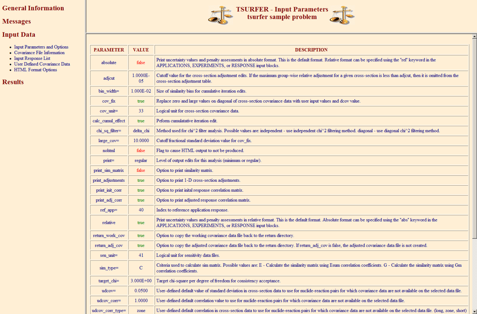
Fig. 6.8.3 Input parameters from TSURFER HTML output.
Selecting Messages will reveal a menu of available messages. Selecting Warning Messages from the Messages section of the menu causes the information shown in Fig. 6.8.4 to appear. The Warning Messages edit contains all warning messages that were generated during the execution of the code. If errors were encountered in the code execution, an Error Messages item would have also been available in the menu under Messages.
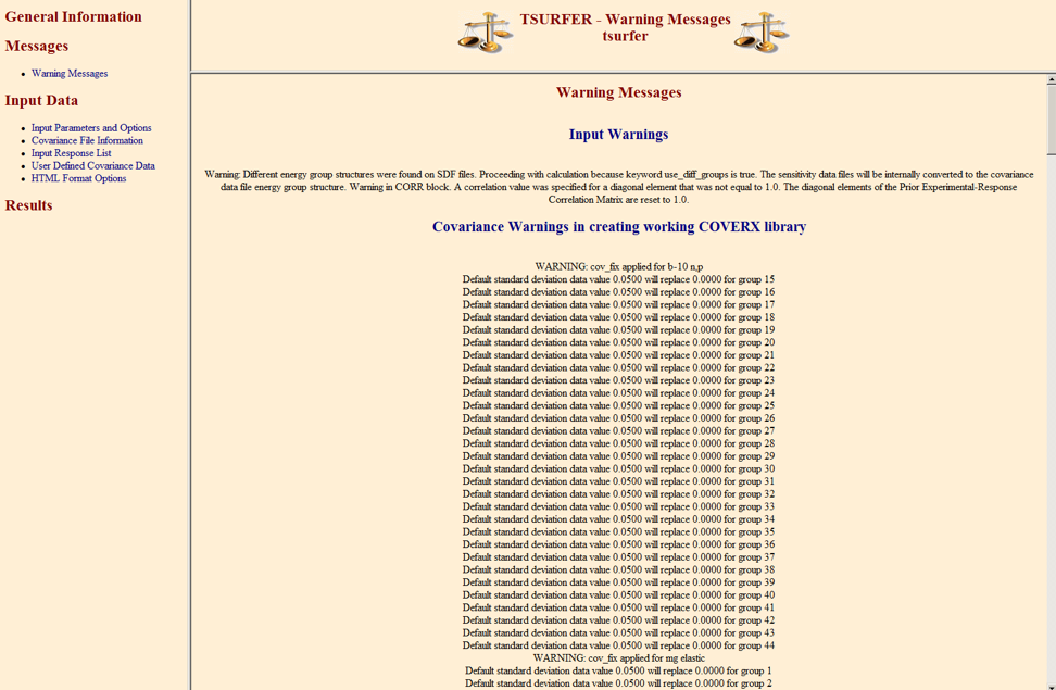
Fig. 6.8.4 Warning messages from TSURFER HTML output.
Selecting Results causes a menu of available results to be revealed. From this menu, selecting Cross-Section Adjustments causes a menu on the right to be revealed. From this menu, nuclide-reaction pairs can be selected to visualize their cross-section adjustments in tabular format. The U-235 nubar adjustments are shown in Fig. 6.8.5.
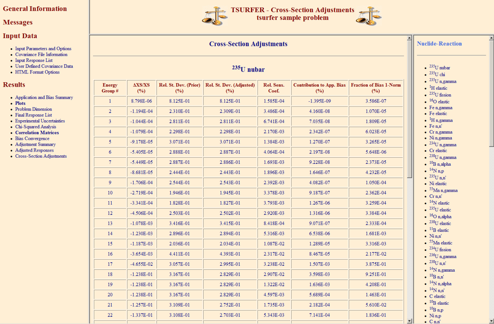
Fig. 6.8.5 Cross-section adjustments from TSURFER HTML output.
Various plots can also be viewed in the TSURFER HTML output. Selecting “Plots” in the Results menu brings up a submenu of various TSURFER plots. The correlation matrices may be viewed by selecting “Correlation Matrices” in the Plots submenu. A Java applet version of Javapeño will appear in the browser window with the correlation matrices preloaded. Data can be added to the plot by double-clicking on the list of available data on the right side of Javapeño. The plot shown in Fig. 6.8.6 was produced with this procedure.
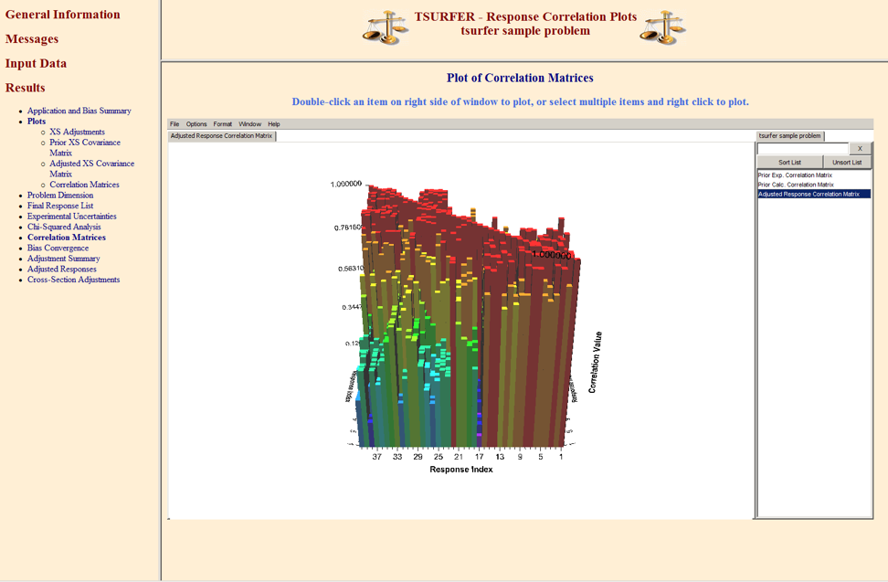
Fig. 6.8.6 Three-dimensional plot of correlation matrix in TSURFER HTML output.
References
- TSURFER-Bri06(1,2)
J. Blair Briggs. International handbook of evaluated criticality safety benchmark experiments. Nuclear Energy Agency, NEA/NSC/DOC (95), 3:l, 2006.
- TSURFER-BHCP99(1,2,3,4,5)
B. L. Broadhead, C. M. Hopper, R. L. Childs, and C. V. Parks. Sensitivity and uncertainty analyses applied to criticality safety validation, methods development. Technical Report, Oak Ridge National Laboratory, Oak Ridge, TN (USA), 1999.
- TSURFER-BHP99(1,2)
B. L. Broadhead, C. M. Hopper, and C. V. Parks. Sensitivity and uncertainty analyses applied to criticality safety validation. Technical Report, Oak Ridge National Laboratory, Oak Ridge, TN (USA), 1999.
- TSURFER-BRH+04(1,2)
B. L. Broadhead, B. T. Rearden, C. M. Hopper, J. J. Wagschal, and C. V. Parks. Sensitivity-and uncertainty-based criticality safety validation techniques. Nuclear science and engineering, 146(3):340–366, 2004.
- TSURFER-Gol04(1,2,3)
Sedat Goluoglu. Sensitivity Analysis Applied to the Validation of the 10 B Capture Reaction in Nuclear Fuel Casks. Technical Report, Oak Ridge National Laboratory, Oak Ridge, TN (USA), 2004.
- TSURFER-Hwa88(1,2)
R. N. Hwang. Topics in data adjustment theory and applications. In Proceedings of the Specialists' Meeting on the Application of Critical Experiments and Operating Data to Core Design via Formal Methods of Cross Section Data Adjustment. Jackson Hole, WY (USA), 9 1988.
- TSURFER-JRCMPR16
E. Juárez Ruiz, R. Cortes Maldonado, and F. Pérez Rodríguez. Relationship between the Inverses of a Matrix and a Submatrix. Computación y Sistemas, 20(2):251–262, July 2016. URL: http://www.cys.cic.ipn.mx/ojs/index.php/CyS/article/view/2083 (visited on 2020-08-10), doi:10.13053/cys-20-2-2083.
- TSURFER-LKH+08(1,2)
R. C. Little, T. Kawano, G. D. Hale, M. T. Pigni, M. Herman, P. Obložinsky, M. L. Williams, M. E. Dunn, G. Arbanas, and D. Wiarda. Low-fidelity Covariance Project. Nuclear Data Sheets, 109(12):2828–2833, 2008. Publisher: Elsevier.
- TSURFER-MWB81(1,2)
R. E. Maerker, J. J. Wagschal, and B. L. Broadhead. Development and demonstration of an advanced methodology for LWR dosimetry applications. Technical Report, Oak Ridge National Laboratory, Oak Ridge, TN (USA), 1981.
- TSURFER-PRR+74
A. Pazy, G. Rakavy, I. Reiss, J. J. Wagschal, Atara Ya’ari, and Y. Yeivin. The role of integral data in neutron cross-section evaluation. Nuclear Science and Engineering, 55(3):280–295, 1974. Publisher: Taylor & Francis.
- TSURFER-PC88(1,2)
W. P. Poenitz and P. J. Collins. Utilization of experimental integral data for the adjustment and uncertainty evaluation of reactor design quantities. In Proceedings of the Specialists' Meeting on the Application of Critical Experiments and Operating Data to Core Design via Formal Methods of Cross Section Data Adjustment. Jackson Hole, WY (USA), 9 1988.
- TSURFER-TTYS88
T. Takeda, M. Takamoto, A. Yoshimura, and K. Shirakata. Adjustment of JENDL-2 Cross Sections and Prediction Accuracy for FBR Core Parameters Using Jupiter Integral Data. In Proceedings of the Specialists' Meeting on the Application of Critical Experiments and Operating Data to Core Design via Formal Methods of Cross Section Data Adjustment. Jackson Hole, WY (USA), 9 1988.
- TSURFER-WML+76
C. R. Weisbin, J. H. Marable, J. L. Lucius, E. M. Oblow, F. R. Mynatt, R. W. Peelle, and F. G. Perey. Application of FORSS sensitivity and uncertainty methodology to fast reactor benchmark analysis. Technical Report, Oak Ridge National Laboratory, Oak Ridge, TN (USA), 1976.
- TSURFER-WBP01(1,2,3)
M. L. Williams, B. L. Broadhead, and C. V. Parks. Eigenvalue sensitivity theory for resonance-shielded cross sections. Nuclear Science and Engineering, 138(2):177–191, 2001.
- TSURFER-Wil86(1,2,3,4,5)
Mark L. Williams. Perturbation theory for nuclear reactor analysis. CRC Press, Inc., 1986.
- TSURFER-WR08(1,2)
Mark L. Williams and Bradley T. Rearden. SCALE-6 Sensitivity/uncertainty methods and covariance data. Nuclear Data Sheets, 109(12):2796–2800, 2008.
- TSURFER-YWMW80
Y. Yeivin, J. J. Wagschal, J. H. Marable, and C. R. Weisbin. Relative Consistency of ENDF/B-IV and-V with Fast Reactor Benchmarks. In Nuclear Cross Sections for Technology: Proceedings of the International Conference on Nuclear Cross Sections for Technology, Held at the University of Tennessee, Knoxville, TN, October 22-26, 1979, volume 594, 182. US Department of Commerce, National Bureau of Standards, 10 1980.