6.2. TSUNAMI-3D: Control Module for Three-Dimensional Cross Section Sensitivity and Uncertainty Analysis for Criticality
K. B. Bekar, T. M. Greene, S. R. Johnson, B. Langley, J. D. McDonnell, W. J. Marshall, C. M. Perfetti, B. T. Rearden, W. A. Wieselquist
ABSTRACT
TSUNAMI-3D (Tools for Sensitivity and Uncertainty Analysis Methodology Implementation in Three Dimensions) is a SCALE control module that facilitates the application of sensitivity and uncertainty analysis theory to criticality safety analysis. In multigroup (MG) mode, TSUNAMI-3D provides for resonance self-shielding of cross section data, calculation of the implicit effects of resonance self-shielding calculations, calculation of forward and adjoint Monte Carlo neutron transport solutions, and calculation of eigenvalue sensitivity coefficients. In continuous-energy (CE) mode, sensitivity coefficients are computed in a single forward Monte Carlo neutron transport calculation for either eigenvalue or generalized reaction rate ratio responses. In both MG and CE modes, the KENO V.a or KENO-VI module is used for transport solvers, and the SAMS module is used to compute and/or create edits of the sensitivity of the calculated responses to the nuclear data used in the calculation as a function of nuclide, reaction type, and energy. SAMS also computes the uncertainty in the calculated responses resulting from uncertainties in the basic nuclear data used in the calculation through energy-dependent cross section covariance matrices. In both MG and CE calculations, a sensitivity data file is produced for use in subsequent analysis.
Version Information
Version 6.2 (2016)
Code Responsible(s): B. T. Rearden, C. M. Perfetti, and L. M. Petrie
The following section acknowledgements appeared in the SCALE 6.2 manual.
The author wishes to acknowledge M. L. Williams, B. L. Broadhead, and K. B. Bekar, of Oak Ridge National Laboratory (ORNL), and R. L. Childs, formerly of ORNL, for their assistance with this work. The support and encouragement of C. M. Hopper, formerly of ORNL, and C. V. Parks and D. E Mueller of ORNL is also appreciated. The continued support of the U.S. Department of Energy Nuclear Criticality Safety Program and the ORNL Laboratory-Directed Research and Development Program is gratefully acknowledged.
6.2.1. Introduction
TSUNAMI-3D (Tools for Sensitivity and Uncertainty Analysis Methodology Implementation in Three Dimensions) is a SCALE control module that facilitates the application of sensitivity and uncertainty theory to criticality safety analysis. The data computed with TSUNAMI-3D are the sensitivity of computed responses (e.g. keff and ratios of reaction rates) to each constituent nuclear data component used in the calculation. The sensitivity data are coupled with cross section uncertainty data, in the form of multigroup (MG) covariance matrices, to produce an uncertainty in the computed responses due to uncertainties in the underlying nuclear data. The group-wise sensitivity data computed with TSUNAMI-3D are stored in a sensitivity data file format (.sdf file) that is suitable for use in data visualization with Fulcrum, similarity assessment with TSUNAMI-IP, and bias assessment with TSURFER.
This manual is intended to provide the user with a detailed reference on code input options and some examples of the application of TSUNAMI-3D to generate sensitivity and uncertainty data. The techniques used in the MG and continuous-energy (CE) versions of TSUNAMI-3D are described in Sect. 6.2.2 and Sect. 6.2.3, respectively. The input for TSUNAMI-3D is presented in Sect. 6.2.4, and the use of TSUNAMI-3D to obtain accurate sensitivity coefficients for several sample problems is given in Sect. 6.2.5. Additional information is provided in the appendix. A new user may wish to review the sample problems and then refer to the input description in Sect. 6.2.4 to obtain specific guidance on preparing input for specific models.
TSUNAMI-3D provides automated, problem-dependent cross sections using the same methods and input as the Criticality Safety Analysis Sequences (CSASs). Although CE calculations with TSUNAMI do not require resonance self-shielding calculations because of its use of CE cross sections, MG TSUNAMI-3D uses self-shielding codes that are similar to those used in MG CSAS calculations. The BONAMIST code computes the sensitivity of resonance self-shielded cross to the input data, the so-called “implicit sensitivities” for MG calculations.
After the cross sections are processed, the MG TSUNAMI-3D-K5 sequence performs two KENO V.a criticality calculations, one forward and one adjoint; the MG TSUNAMI-3D-K6 sequence performs two KENO-VI calculations. Finally, the sequence calls the SAMS module to calculate the sensitivity coefficients that indicate the sensitivity of the computed responses to changes in the cross sections and the uncertainty in the computed responses that is due to uncertainties in the basic nuclear data. SAMS prints energy-integrated sensitivity coefficients and their statistical uncertainties to the SCALE output file and generates a separate data file containing the energy-dependent sensitivity coefficients. CE calculations in TSUNAMI do not require a separate adjoint criticality calculation; instead, they calculate sensitivity coefficients and produce a sensitivity data file during a single forward simulation. The SAMS module is used to print user output for CE calculations.
Choosing poor values for any of several adjustable parameters in TSUNAMI inputs may result in inaccurate sensitivity coefficient estimates; thus, users are advised to always compare their calculated sensitivity coefficients to reference values to verify the suitability of their TSUNAMI input parameters. Sect. 6.2.5 describes the direct perturbation approach for generating reference sensitivity coefficients for the total cross section of nuclides in a system. It is difficult to calculate high fidelity, energy-dependent, reference sensitivity coefficients using direct perturbation (although possible using stochastic sampling of cross section data), but at the minimum users are advised to verify the accuracy of TSUNAMI-produced total nuclide sensitivity coefficients for all key nuclides in their application.
6.2.2. Multigroup TSUNAMI-3D Techniques
TSUNAMI-3D is a SCALE control module. As such, its primary function is to control a sequence of calculations that are performed by other codes. A thorough theoretical development of MG eigenvalue sensitivity theory is described in the SAMS section of the SCALE documentation. Currently, two computational sequences are available with TSUNAMI-3D: TSUNAMI-3D-K5 and TSUNAMI-3D-K6. The input for TSUNAMI-3D-K5 is very similar to that used for CSAS5 and the input for TSUNAMI-3D-K6 is very similar to that of CSAS6. TSUNAMI-3D uses the same material and cell data input as all other SCALE sequences. TSUNAMI-3D can calculate eigenvalue sensitivity coefficients using either MG or CE Monte Carlo simulations, but the theoretical approaches for each calculation mode differ greatly. MG TSUNAMI-3D techniques will be discussed in this section, and CE TSUNAMI-3D calculations will be discussed in Sect. 6.2.3. The control sequences available in MG TSUNAMI-3D are summarized in Table 6.2.1, where the functional modules that are executed are also shown. A general flow diagram of MG TSUNAMI-3D is shown in Fig. 6.2.1.
Control sequence |
Functional modules executed by the control module |
||||
TSUNAMI-3 D-K5 |
XSProc |
KENO V.a forward |
KENO V.a adjoint |
BONAMIST |
SAMS5 |
TSUNAMI-3 D-K6 |
XSProc |
KENO-VI forward |
KENO-VI adjoint |
BONAMIST |
SAMS6 |
TSUNAMI-3D and many other SCALE sequences apply a standardized procedure to provide appropriate cross sections for the calculation. This procedure is carried out by routines of the XSProc module, which generate number densities and related information, prepare geometry data for resonance self-shielding and flux-weighting cell calculations, and create data input files for the cross section processing codes.
By default, the MG TSUNAMI-3D sequence performs cross-section processing with XSProc, exercising all available options there, performs the forward and adjoint KENO calculations, calls BONAMIST to produce implicit sensitivity coefficients, then calls SAMS to produce sensitivity and uncertainty output and sdf files. Optional sequence level parameters can be used to change methods applied in resonance self-shielding and exclude the implicit sensitivity calculation, which are detailed later in this document.
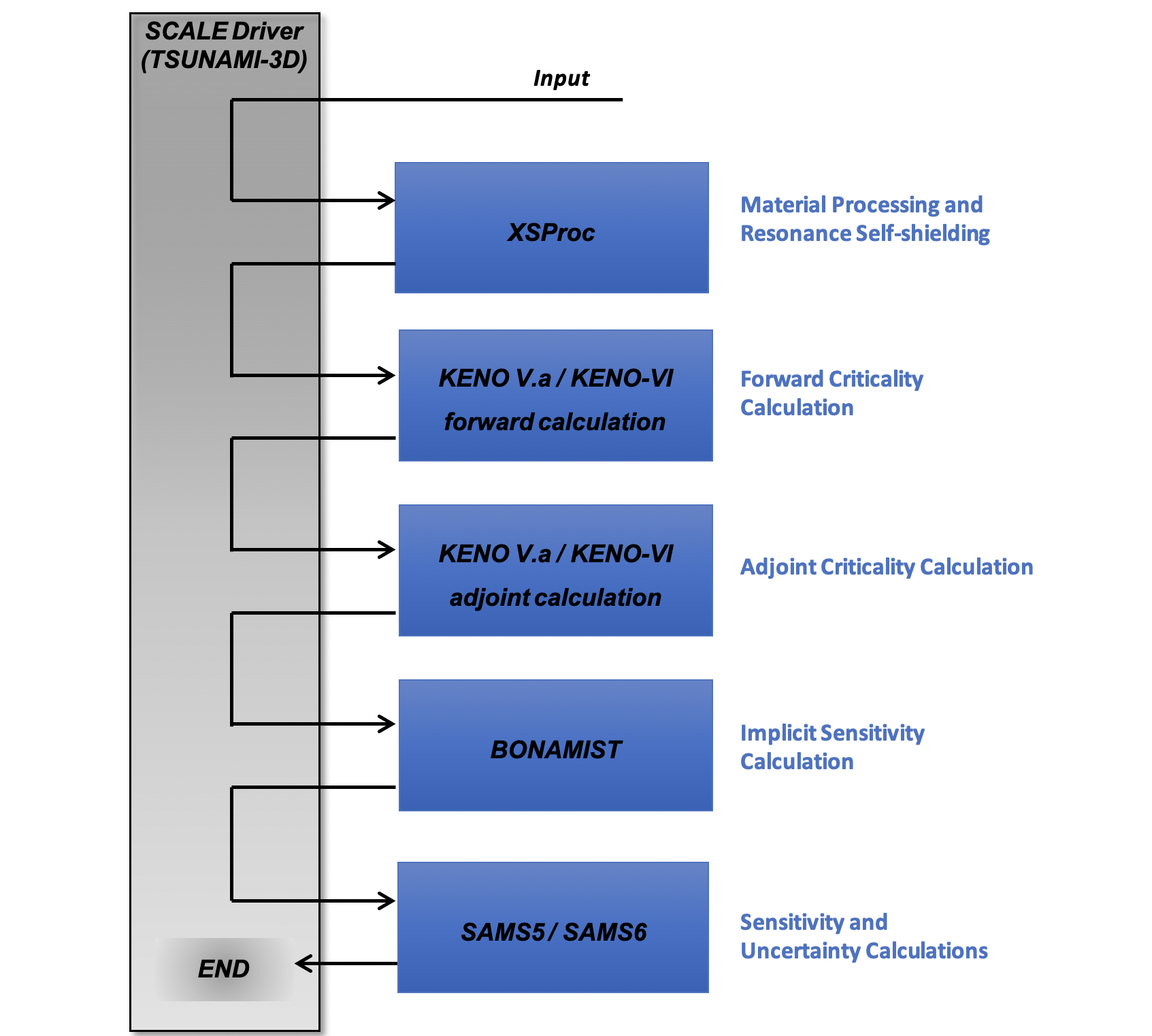
Fig. 6.2.1 General flow diagram of MG TSUNAMI-3D.
Once the appropriate AMPX libraries are prepared, TSUNAMI-3D prepares KENO V.a or KENO-VI inputs for forward and adjoint calculations from the criticality model provided by the user. The input requirements for the KENO V.a input sections are identical to those for the CSAS5 sequence, with some optional additional data. Also, the input requirements for the KENO-VI are identical to those for CSAS6, with some optional additional data. Additional input is prepared for the SAMS module using an optional user-defined input block for SAMS. TSUNAMI-3D executes forward and adjoint KENO calculations, generates implicit sensitivity data with BONAMIST, and then executes the SAMS module to compute the sensitivity and uncertainty data using the data accumulated from the codes previously executed in the sequence. Details concerning calculation of sensitivity and uncertainty data using MG forward and adjoint calculations are provided in the SAMS chapter of the SCALE manual. Of particular interest, the filename.sdf file, where filename is the name of the input file less any extensions, contains energy-dependent sensitivity coefficients. SCALE returns this file to the same directory as the input file.
The XSProc module is responsible for reading the standard composition data and other engineering-type specifications, including volume fraction or percent theoretical density, temperature, and isotopic distribution as well as the unit cell data. The techniques used in the XSProc module and their applications and limitations are discussed in the XSProc chapter. The input data for XSProc is the same for all analytical sequences available through TSUNAMI-3D, TSUNAMI-1D, CSAS, and many other SCALE sequences.
6.2.3. Continuous-Energy TSUNAMI-3D Techniques
Like MG TSUNAMI-3D, the CE TSUNAMI-3D capability is a control module that uses codes within the SCALE code package to calculate eigenvalue sensitivity coefficients and other information for models of eigenvalue problems. The CE and MG TSUNAMI-3D calculations differ dramatically in their approach for calculating sensitivity coefficients and as a result have different user interfaces. CE TSUNAMI calculations are automatically enabled when the user selects a CE cross-section library.
6.2.3.1. CE TSUNAMI methodology
CE TSUNAMI currently contains two separate approaches for performing eigenvalue sensitivity coefficient calculations: Iterated Fission Probability (IFP) approach and Contributon-Linked eigenvalue sensitivity/Uncertainty estimation via Tracklength importance Characterization (CLUTCH) approach. Both IFP and CLUTCH calculate sensitivity coefficients during a single forward Monte Carlo (KENO) simulation. Unlike MG TSUNAMI-3D, IFP and CLUTCH do not require the simulation of adjoint histories, calculation of angular flux moments using a flux mesh, volume calculations, or treatment of implicit sensitivity effects. The theoretical background of each method is discussed in detail in the following sections. IFP is often easier to use than CLUTCH, but CLUTCH has greater computational efficiency and a lower memory footprint.
6.2.3.1.1. IFP methodology
The IFP methodology, developed by Hurwitz in the 1940s and 1950s, determines the importance of events during a particle history using the notion that an event’s importance is proportional to the number of neutrons descended from the original event that are present in the system during some future generation. [3d1], [3d2] In practice, the IFP method requires storing reaction rate tallies for particles for some number of generations until the average population of their descendants in the system, the “asymptotic population,” is obtained. This process is illustrated in Fig. 6.2.2. Once obtained, the asymptotic population of the original neutron is used to weight reaction rate tallies for that neutron and to produce sensitivity coefficient estimates via the first-order perturbation equation. The number of fission neutrons created by progenitor \(p\)’s asymptotic population,
takes the place of the adjoint flux \(\phi^\ast\) in the first-order perturbation equations.
A number of generations, referred to as the “latent generations,” must be skipped before calculating the asymptotic population for an event to guarantee that the progeny of the event have had sufficient time to impact all regions in the system and to converge to a true estimate of the asymptotic population. The number of latent generations required to calculate accurate sensitivity coefficients varies based on the complexity of the system and the desired sensitivity coefficient fidelity, but in general 20 generations is a conservative number of latent generations to ensure convergence to the asymptotic population. (Note that the current default in TSUNAMI-3D is 5 latent generations.) The IFP method is useful for benchmarking the accuracy of other sensitivity coefficient methods and is very easy to use because the only assumption of the IFP method (besides the standard CE Monte Carlo and first order perturbation theory assumptions) is that the asymptotic population that is reached after the chosen number of latent generations is representative of the importance of the original event. Thus a user who is new to sensitivity methods can assume a conservative number of latent generations and can use the IFP method to accurately calculate sensitivity coefficients for a system so long as the user’s computer has sufficient computational memory for the simulation.
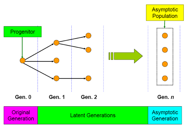
Fig. 6.2.2 Illustration of the Iterated Fission Probability process.
The IFP method requires storage of region-, isotope-, reaction-, and energy-dependent reaction rates for every particle for the specified number of latent generations. Complex problems can require simulating tens of thousands or hundreds of thousands of particles during each generation, and IFP simulations for these systems can easily require many gigabytes of computational memory storage. The IFP implementation in TSUNAMI-3D makes use of dynamic memory allocation to minimize memory requirements, but the method frequently produces large memory footprints despite these optimizations. The IFP memory requirements are proportional to the number of latent generations used in the calculations, and perhaps the best approach for minimizing the memory requirements of the IFP method is to minimize the number of latent generations used in a calculation. Twenty is typically a conservative number of latent generations, and it is recommended that the user always use as few latent generations as possible for IFP simulations. The five latent generations that IFP assumes by default is a reasonable starting guess, but users should compare IFP nuclide sensitivity coefficients with direct perturbation sensitivities to determine if they need to use more or fewer latent generations. Determining the adequate number of latent generations can be done by starting with a small number of latent generations and slowly increasing the number until the IFP-calculated sensitivity coefficients agree well with reference sensitivities. The memory requirements of the IFP method are also proportional to the number of particles used in each generation (NPG), and high-memory simulations can decrease NPG to decrease the memory requirements of the IFP method. This should be done with caution because making NPG too small can affect the fission source convergence and thus can produce poor tally Monte Carlo variance estimates.
The integration of the Shift Monte Carlo transport code has made possible the parallelization of the IFP method, so that the large amount of memory required can be distributed among several available processors. Note that this parallelism for IFP is only available when using the Shift transport code, and it is not available through KENO.
6.2.3.1.2. CLUTCH methodology
The CLUTCH method was developed by Perfetti in 2012, based in part on the Contributon theory explored by M. L. Williams of ORNL, to produce an accurate and efficient means for calculating eigenvalue sensitivity coefficients with a small computational memory footprint. [3d3] Like the IFP method, CLUTCH calculates sensitivities during a single forward Monte Carlo calculation and does not require tallying angular flux moments. Instead, the CLUTCH method calculates the importance of events during a particle’s lifetime by examining how many fission neutrons are created by that particle after those events occur. Consider a neutron source Q that is equal to the fission source of a system:
Multiplying this source by the adjoint flux and integrating over phase space gives
Consider now a neutron emitted in phase space \(\tau_{s}\) such that \(Q\left( \tau_{s} \right) = Q_{s}\ \delta(\tau - \tau_{s})\). This source definition reduces Eq. (6.2.3) and allows the importance of the neutron in phase space \(\tau_{s}\) to be calculated by
where the transfer function \(G\left( \tau_{s} \rightarrow r \right)\) is equal to the expected number of fission neutrons generated in all energies and directions at \(r\) due to a neutron emitted at phase space \(\tau_{s}\) and is given by
where \(\phi\left(r, E, \Omega \mid Q\left(\tau_{s}\right)\right)\) is the flux created in phase space \((r,E,\Omega)\) given the source \(Q\left( \tau_{s} \right)\). The weighting function \(F^{*}\left( r \right)\) is defined to be equal to the expected importance generated by a fission neutron emitted at \(r\) and is given by
In practice, the CLUTCH method calculates the integral of \(G\left( \tau_{s} \rightarrow r \right)\), weighted by \(F^{*}\left( r \right)\), to calculate the importance of every event in a particle’s lifetime. For example, the importance of a scattering event would be determined by tallying how many fission neutrons, weighted by the value of \(F^{*}\left( r \right)\) at the sites where they are born, are created by the neutron that emerges from the scattering collision. The CLUTCH method cannot calculate the importance of events until after the particle that caused these events dies, which requires that CLUTCH store reaction rate information for every collision that a particle undergoes during its lifetime. This is a manageable amount of information because these tallies are not energy dependent (a particle’s energy is constant between any two collisions) and because this information can be deleted once the particle dies. In contrast, the IFP method requires much more memory because it stores energy-dependent reaction rate tallies for every particle for the number of latent generations.
The only assumption made by the CLUTCH method (besides the standard CE Monte Carlo assumptions) is that \(F^{*}\left( r \right)\) provides an accurate estimate of the average importance of fission neutrons at \(r\). The current approach for calculating \(F^{*}\left( r \right)\) takes advantage of the definition of the unconstrained fission spectrum sensitivity coefficient, which is given by
where \(D\) is the adjoint-weighted fission source for the system. The right-most integral of Eq. (6.2.7) is recognized as the definition of \(F^{*}\left( r \right)\) in Eq. (6.2.6) and the terms in Eq. (6.2.7) can be rearranged to define \(F^{*}\left( r \right)\) as
This approach assumes that the energy spectrum of neutrons emitted from a fission event is not strongly dependent on the parent isotope or the energy of the neutron causing the fission. The current CLUTCH implementation tallies the unconstrained chi sensitivity in the numerator of Eq. (6.2.8) during the inactive generations to estimate \(F^{*}\left( r \right)\) for the active generation sensitivity coefficient calculations. The spatial dependence of \(F^{*}\left( r \right)\) is currently accounted for by calculating and storing \(F^{*}\left( r \right)\) on a spatial mesh, although kernel density estimators might be used in the future to store \(F^{*}\left( r \right)\) using spatially continuous functional representations. [3d4] Because \(F^{*}\left( r \right)\) is only nonzero for regions containing fissionable material, the \(F^{*}\left( r \right)\) mesh used in a CE TSUNAMI calculation must only encompass all fissionable material in the system, rather than the entire system as required by MG TSUNAMI. The \(D\) term in Eq. (6.2.8) can be ignored because it is constant for all regions in a problem and is cancelled out by the presence of \(F^{*}\left( r \right)\) terms in both the numerator and denominator of the first-order perturbation equation. The denominator in Eq. (6.2.8) is simply the total weight of fission neutrons born in each \(F^{*}\left( r \right)\) mesh region, which must also be tallied during the inactive generations.
Because \(F^{*}\left( r \right)\) describes the contribution to the chi sensitivity that is created per fission neutron born at a point, a converged fission source is not required to begin \(F^{*}\left( r \right)\) calculations; thus, \(F^{*}\left( r \right)\) tallies begin during the inactive generations of Monte Carlo simulations to obtain useful information from the typically discarded inactive particle histories. The fission source must converge well enough during the inactive generations so that \(F^{*}\left( r \right)\) is tallied in all fissile regions to a desired statistical uncertainty, and it is sometimes necessary to simulate extra inactive generations to allow \(F^{*}\left( r \right)\) tallies to fully converge; however, the ability to begin \(F^{*}\left( r \right)\) tallies before the fission source is converged essentially provides “free” tallies while the fission source is converging.
Although several approaches exist for calculating the unconstrained chi sensitivity coefficients needed to calculate \(F^{*}\left( r \right)\), an IFP-based approach has been determined to be the best approach. [3d3] Although the IFP method can produce large memory footprints for full sensitivity coefficient calculations, the amount of memory required by the method to calculate unconstrained chi sensitivity coefficients and \(F^{*}\left( r \right)\) is generally negligible. The spatial dependence of \(F^{*}(r)\) is currently described using a spatial mesh, and an interval of 1 to 2 cm mesh is typically sufficiently refined to obtain accurate \(F^{*}\left( r \right)\) estimates. Users should simulate at least on the order of 50 to 100 inactive histories per mesh interval to allow for sufficient \(F^{*}(r)\) convergence; sometimes this necessitates simulating a large number of additional inactive histories/generations.
6.2.3.2. CE TSUNAMI Generalized Perturbation Theory capability
The CLUTCH and IFP methods were combined in 2013 by Perfetti to enable sensitivity calculations for generalized neutronic response ratios. [3d5] This Generalized Perturbation Theory (GPT) capability is known as the GEneralized Adjoint Responses in Monte Carlo (GEAR-MC) method. Applications for GPT sensitivity coefficients differ from the traditional criticality safety applications of TSUNAMI, and may include S/U analyses for multigroup cross sections that are produced by a continuous-energy Monte Carlo code, the relative power of pins in a LWR, or ratios of foil activities in an irradiation experiment.
Two approaches for performing the GEAR-MC method have been included in this release as demonstration capabilities. One implementation relies heavily on the IFP method for sensitivity calculations and is therefore subject to the long runtimes and large memory footprint that may be encountered when using the IFP method. The other implementation does not use the IFP method when calculating sensitivities. Instead, it uses only the CLUTCH method with an \(F^{*}(r)\) mesh that has been modified for performing generalized response sensitivity calculations. Because it does not use the IFP method except for calculating the \(F^{*}(r)\) function, this approach typically produces a significantly lower memory footprint than the first GEAR-MC implementation and can be performed in a parallel environment. [3d6] Both approaches are experimental capabilities and have been included in this release to demonstrate the expanding SCALE S/U capabilities. For the CLUTCH-only GPT, the current format for inputting response information allows for the sensitivity calculations for a single response in each sensitivity calculation. For GPT via CLUTCH and IFP, multiple responses may be defined.
Rather than calculating eigenvalue sensitivities, the GEAR-MC method calculates the sensitivity of a response, \(R\), to perturbations or uncertainties in the system parameters. The generalized response sensitivity coefficient for the system parameter \(\Sigma_{x}\) is defined as
The GEAR-MC method calculates sensitivities of responses that are defined as ratios of neutron reaction rates integrated over some region of phase space such that
where \(\Sigma_{1}\) and \(\Sigma_{2}\) are nuclear cross sections. The reaction rates in Eq. (6.2.10) can be isotope- or material-dependent reaction rates and can also represent neutron flux responses if \(\Sigma = 1\). The fractional change in \(R\) due to a perturbation \(\delta\Sigma_{x}\) to the system parameter \(\Sigma_{x}\) is given by
The first term in Eq. (6.2.11) is known as the “direct effect term” and describes how perturbations in \(\Sigma_{x}\) affect the response function of the response reaction rates. The second term, known as the “indirect effect term,” describes how perturbations affect the neutron flux spectrum in the response region. [3d7] Calculating the sensitivity of the response to the direct effect term is relatively simple and involves tallying the fraction of the total numerator and denominator responses that is generated for each energy, region, isotope, and material in the response region(s). For example, consider a response that is defined as the ratio of the energy-integrated fission rate to the energy-integrated capture rate in a uranium fuel pin. The direct effect sensitivity of this response to the thermal fission cross section is simply the fraction of the fission reaction rate in the pin that is caused by neutrons with thermal energies.
The indirect effect term in Eq. (6.2.11) cannot be calculated as simply as the direct effect term and has historically posed a greater challenge. The GEAR-MC method offers an approach for calculating the indirect effect term during a single, unperturbed Monte Carlo transport calculation. The neutron balance equation for an eigenvalue problem is given by
where \(L\) is the neutron loss operator and \(P\) is the fission neutron production operator. The change induced in the neutron balance equation in response to a first-order perturbation is given by
Consider now the generalized adjoint balance equation
where \(L^{*}\) is the adjoint loss operator, \(P^{*}\) is the adjoint fission neutron production operator, \(S^{*}\) is a source of importance for the response that is defined such that \(\left\langle\phi S^{*}\right\rangle=0\), and \(\Gamma^{*}\) is the generalized importance function that provides the solution to this equation.7 Multiplying Eq. (6.2.13) and Eq. (6.2.14) by \(\Gamma^{*}\) and \(\delta \phi\), respectively, and taking the inner product gives, respectively,
and
The source of adjoint importance in Eq. (6.2.16) is defined to conveniently provide an expression for the indirect effect term. Defining \(S^{*}\) as
and applying the adjoint property allows Eq. (6.2.15) and Eq. (6.2.17) to be combined to express the indirect effect term as
Eq. (6.2.18) is usually equal to zero because \(\Gamma^{*}\) is typically orthogonal to \(P \phi\). The effect of this orthogonality can be interpreted in a more physical manner by realizing that perturbations to the eigenvalue of a system do not alter the steady-state neutron flux shape or spectrum of the system. As a result, perturbations affect the response numerator and denominator terms equally.
The GEAR-MC methodology uses Eq. (6.2.14) and Eq. (6.2.18) to calculate the generalized importance function \(\Gamma^{*}\) for neutrons during a single forward Monte Carlo simulation, thus enabling the calculation of the indirect effect term in Eq. (6.2.11). and thus sensitivity coefficients for generalized responses using GPT. The approach developed for calculating \(\Gamma^{*}\) is similar to the approach used by the CLUTCH method for calculating eigenvalue sensitivity coefficients.
Assuming that the fission production term, \(\lambda P \phi\), in Eq. (6.2.12) is the sole source of neutron production in a system, \(Q\), multiplying Eq. (6.2.12) and Eq. (6.2.14) by \(\Gamma^{*}\) and \(\phi\), respectively, and integrating over all phase space gives
and
Nonfission neutron production reactions, such as (n,Xn) reactions, are included in the \(L^{*}\) adjoint loss term in Eq. (6.2.20). Combining Eq. (6.2.19) and Eq. (6.2.20). and using the adjoint property gives
The terms in Eq. (6.2.21) are all equal to zero in inner product space, but it can be used to extract information about the importance of events by considering the neutron source to be a single neutron traveling through the phase space \(\tau_{s}\), such as a neutron entering or leaving a collision at some point. This concept is used similarly in Williams’ Contributon theory for calculating eigenvalue sensitivity coefficients and assumes that
where \(Q_{s}\) is the source strength for this neutron. [3d8], [3d9] Substituting Eq. (6.2.22) into Eq. (6.2.21) produces an expression for the generalized importance function at \(\tau_{s}\):
where \(\phi(\tau_{s} \rightarrow r)\) is the neutron flux created at \(r\) by the neutron originating at \(\tau_{s}\). The two terms on the right-hand side of Eq. (6.2.21) and Eq. (6.2.23) represent the intragenerational and intergenerational effects of an event on the importance of a particle, respectively. The intragenerational effect term describes how much importance the neutron in phase space \(\tau_{s}\) generates in the response region(s) during its lifetime; the intergenerational effect term describes how many fission neutrons this neutron creates and how much importance these fission neutrons will generate in future generations. The intragenerational term can be determined by tallying the amount of flux generated in the response region(s) and weighted by \(S^{*}\left( r \right)\) from Eq. (6.2.17) from the time the particle enters phase space \(\tau_{s}\) until its death. Thus the intragenerational term is given by
The approach for calculating the intragenerational importance term in Eq. (6.2.24) is similar to the approach used by the CLUTCH method during eigenvalue sensitivity coefficient calculations and requires storing tracklength information for each collision that a particle enters and determining the importance of that collision after the particle dies. The presence of both positive and negative terms in Eq. (6.2.24) allows a single event to generate either a positive or negative importance. The intergenerational contribution to the importance function can be calculated by tallying the cumulative score of \(S^{*}\left( r \right)\phi(\tau_{s} \rightarrow r)\) that is generated by the particle’s daughter fission neutrons, or “progeny,” over some number of generations. The GEAR-MC method estimates the intergenerational importance by summing the intragenerational importance, \(\Gamma_{i}^{*}\), generated by the fission production, \(F_{i}\), of neutrons in the \(i\)th generation of a fission chain over some number of generations:
This approach is used similarly by the IFP approach for calculating the importance of events during eigenvalue sensitivity calculations, except that the IFP method tallies the importance only one time after the daughter neutrons have established an asymptotic population in the system. The \(\delta \lambda\) term in Eq. (6.2.18). demands that the \(\left\langle\Gamma^{*} P \phi\right\rangle\) term be equal to zero, which causes the \(\Gamma_{i}^{*}F_{i}\) terms in Eq. (6.2.25) to approach zero as \(i\) approaches infinity; therefore, the intergenerational importance term is obtained by taking the sum of the \(\Gamma_{i}^{*}F_{i}\) terms as they asymptotically approach zero.
6.2.3.3. CE TSUNAMI sequence description
The code flow of CE calculations with TSUNAMI is significantly simpler than the flow of MG TSUNAMI because CE Monte Carlo does not require resonance self-shielding of MG cross sections or the calculation of implicit sensitivity coefficients and calculates sensitivity coefficients during a single forward calculation. The CE control sequences available in TSUNAMI are summarized in Table 6.2.2, where the functional modules executed are also shown. A general flow diagram of a CE calculation with TSUNAMI is shown in Fig. 6.2.3.
Control sequence |
Functional modules executed by the control module |
|
TSUNAMI-3D-K5 |
KENO V.a |
SAMS5 |
TSUNAMI-3D-K5-SHIFT |
Shift |
SAMS5 |
TSUNAMI-3D-K6 |
KENO-VI |
SAMS6 |
TSUNAMI-3D-K6-SHIFT |
Shift |
SAMS6 |
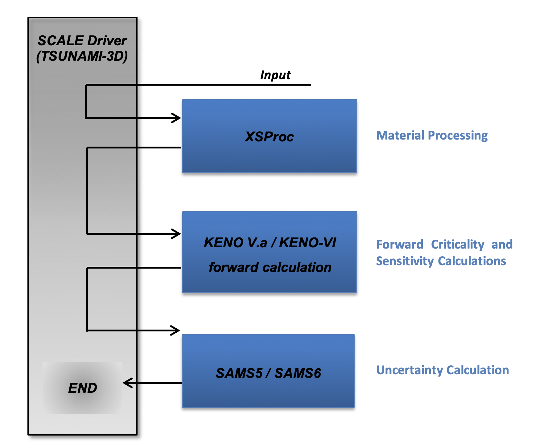
Fig. 6.2.3 General flow diagram of CE TSUNAMI-3D.
Eigenvalue sensitivity coefficients are calculated during the KENO or Shift Monte Carlo transport calculation, and the energy-dependent sensitivity coefficients are summarized in a sensitivity data file (sdf). The SAMS module then uses the .sdf file produced and cross section covariance data to complete the eigenvalue uncertainty analysis for the problem and estimate the data-induced eigenvalue uncertainty.
6.2.4. TSUNAMI-3D Input Description
The input for TSUNAMI-3D is designed to be very compatible with those used for the CSAS criticality safety analysis sequences. Given a CSAS input, MG TSUNAMI-3D calculations only require several input modifications to obtain adequate flux solutions, and CE TSUNAMI calculations require as little as one additional parameter. Additional optional input may be added to control the sensitivity calculations.
The input to TSUNAMI-3D consists of an input title, SCALE analytical sequence specification record, SCALE XSProc data, KENO V.a or KENO-VI input descriptions with some additional optional parameter data, and optional sensitivity and uncertainty data. These data are processed using the SCALE free-form reading routines, which allow alphanumeric data, floating-point data, and integer data to be entered in an unstructured manner. The input is not case sensitive, so either upper- or lowercase letters may be used. A maximum of 252 columns per line may be used for input, although some exceptions for this rule exist, such as the 80 character title data. Data can usually start or end in any column with a few exceptions. As an example, the word END beginning in column 1 and followed by two blank spaces will end the problem, any data following will be ignored. Each data entry must be followed by one or more blanks to terminate the data entry. For numeric data, either a comma or a blank can be used to terminate each data entry. Integers may be entered for floating values. For example, 10 will be interpreted as 10.0. Imbedded blanks are not allowed within a data entry unless an E precedes a single blank as in an unsigned exponent in a floating-point number. For example, 1.0E 4 would be correctly interpreted as 1.0 \(\times\) 104.
6.2.4.1. Analytical sequence specification record
The analytical sequence specification begins in column 1 of the first line of the input file and must contain the following:
=TSUNAMI-3D-K5
This sequence is used for sensitivity and uncertainty calculations with KENO V.a.
=TSUNAMI-3D-K6
This sequence is used for sensitivity and uncertainty calculations with KENO-VI.
Either analytical sequence specification may have -shift appended
in order to use the Shift Monte Carlo transport code.
(Namely, tsunami-3d-k5-shift or tsunami-3d-k6-shift.)
Optional keyword input may be entered after the analytical sequence specification record. These keywords are
PARM=CHECK PARM=CHK |
This option allows the input data to be read and checked without executing any functional modules. |
Note
The following PARM settings only apply to MG calculations and are ignored for CE calculations:
- PARM=SIZE=n
The amount of memory requested in four-byte words may be set with this entry. The default value for n is 20000000. This value only affects calculations in BONAMIST, where this value of the SIZE parameter is used for allocation of storage for the derivatives. Please see the documentation on BONAMIST in the Sensitivity Utility Modules chapter for more details. All other codes use dynamic memory allocation and this value has no effect.
- PARM=BONAMIST
This is the default configuration for MG TSUNAMI-3D calculations. XSProc is used with BONAMI and CENTRM for cross section processing. Implicit sensitivities are produced with BONAMIST.
- PARM=CENTRM
XSProc is used with BONAMI and CENTRM for cross section processing, but BONAMIST is not run. MG TSUNAMI-3D calculations with PARM=CENTRM do not account for contributions by implicit sensitivity effects, and should be used with caution.
- PARM=BONAMI
XSProc is used with BONAMI for cross section processing, but BONAMIST is not run. MG TSUNAMI-3D calculations with PARM=BONAMI do not account for contributions by implicit sensitivity effects, and should be used with caution.
- PARM=2REGION
XSProc (with BONAMI and CENTRM) use Dancoff factors to compute neutron escape probabilities for an accelerated, yet more approximate, CENTRM calculation. Implicit sensitivities are computed with BONAMIST.
Multiple parameters can be used simultaneously by enclosing them in parentheses and separating them with commas such as PARM=(SIZE=2000000, CHECK).
6.2.4.2. Title data
A title, a character string, must be entered as the second line of the input file. The syntax for the title is a string of characters with a length of up to 80 characters, including blanks.
6.2.4.3. XSProc Execution
XSProc reads the standard composition specification data for MG and CE and the unit cell geometry specifications for MG resonance self-shielding calculations. CE TSUNAMI calculations do not require the specification of unit cells. Please see chapters on the Material Information Processor for input specifications. The cross section data library that is to be used by TSUNAMI must also be entered as the third line of the TSUNAMI input; a list of the currently available libraries are listed in the table Standard SCALE cross section libraries of the XSLIB chapter.
6.2.4.4. KENO V.A or KENO-VI problem description
The KENO V.a or KENO-VI problem description follows the Material Input Processor section in the TSUNAMI-3D input. The input for KENO V.a and KENO-VI in TSUNAMI-3D is very similar to that described in section KENO V.a Data Guide in chapter KENO V.a or section KENO-VI Data Guide in the KENO-VI chapter, with only a few differences in the default values for the parameter data and a few additional parameters to control the adjoint criticality calculation. Otherwise, geometry, array, biasing, boundary, start, and plot data are entered exactly as described for KENO. Default parameter values for MG TSUNAMI-3D that are different from those used for other MG KENO calculations are shown in Table 6.2.3. Parameters that are unique to TSUNAMI-3D and are used to control to the MG adjoint calculation are shown in Table 6.2.4. These adjoint parameters are optional and can be entered with other parameters in the standard READ PARAMETER input block in KENO problem description. Parameters that are unique to CE TSUNAMI-3D are shown in Table 6.2.5; these parameters can also be entered in the KENO READ PARAMETER input block.
Several features were added to KENO V.a and KENO-VI to allow the calculation of sensitivity coefficients from the MG Monte Carlo analysis. One significant addition is the calculation of neutron flux moments and/or angular fluxes, both of which give directional components to the neutron flux solution required to compute the sensitivity of keff to scattering cross sections. Another significant addition is the ability to compute fluxes that are subdivided over a cubic mesh or Cartesian spatial grid. These mesh fluxes simplify the accurate computation of the product of the forward and adjoint flux solutions, sometimes called the “inner product.” Both of the flux moments and the spatial flux mesh options must be correctly applied to obtain accurate sensitivity coefficients. Generally, the refinement of the flux mesh to sufficiently small intervals to capture relevant spatial effects while maintaining a manageable memory footprint is the most challenging aspect of performing MG calculations with TSUNAMI-3D.
Important
It is important to note that TSUNAMI-3D provides no default mesh for these flux tallies, and the user must input a mesh using either the MSH parameter or a GridGeometry input to access this feature.
New input data that aid in the accurate calculation of sensitivity coefficients are the parameter inputs: NQD, PNM, MFX, MSH, TFM, APG, AGN, ABK, ASG, CET, CFP, CGD, FST, NNC, NMA, NMT, DNC, DMA, DMT, NMX, NMN, DMX, and DMN. Thus, these parameters may require modification when using TSUNAMI-3D. The READ GRID block of KENO input is used with MSH to input the planar grid for MG TSUNAMI-3D calculations and also to input the spatial grid for the calculation and storage of \(F^{*}\left( r \right)\) for CE TSUNAMI calculations. Also, if using the coordinate transform for angular flux or flux moment calculations, use of the optional CENTER modifier in the KENO geometry input may be required. Users should note that when using the xlinear, ylinear, or zlinear options in the READ GRID block that KENO checks to determine whether the boundaries of each grid coincide with the global unit boundaries. If any planes in the grid boundaries are identical to the planes used in the global boundary, then KENO will extend the outermost plane in that grid by a distance equal to one-tenth of the grid mesh interval to ensure that the grid mesh covers the entire geometry.
Some KENO parameters (e.g., SCD, MFX, CDS, GFX, and CGD) may be used to assign user provided grid definitions for use with specific tallies. These are described in Sect. 8.1.3.3 of the SCALE KENO chapter. Grid IDs in the READ GRID blocks should be limited to no more than 4 integer characters (i.e., \(1 \leq \text{ID} \leq 9999\)).
Parameter |
Default value for TSUNAMI-3D |
Default value for KENO in CSAS Sequences or as stand-alone code |
Description |
|---|---|---|---|
CFX |
YES |
NO |
Collect fluxes |
GEN |
550 |
203 |
Number of generations to be run |
NSK |
50 |
3 |
Number of generations to be omitted when collecting results |
PNM |
3 |
0 |
Highest order of flux moments tallies |
TFM |
YES |
NO |
Perform coordinate transform for flux moment and angular flux calculations |
Parameter |
Default value for TSUNAMI-3D |
Corresponding KENO parameter |
Description |
|---|---|---|---|
ABK |
APG \(\times\) 2 |
NBK |
Number of positions in the neutron bank for the adjoint calculation |
AGN |
GEN - NSK + ASK |
GEN |
Number of generations to be run for the adjoint calculation - default value produces the same number of active generations as the forward calculation |
APG |
NPG \(\times\) 3 |
NPG |
Number of particles per generation |
ASG |
SIG (default SIG=0) |
SIG |
if > 0.0, this is the standard deviation at which the adjoint problem will terminate |
ASK |
NSK \(\times\) 3 |
NSK |
Number of generations to be omitted when collecting results for the adjoint calculation |
MG TSUNAMI sensitivity coefficient estimates can be very sensitive to the values of a problem’s input parameters, and users should always check the accuracy of their sensitivity coefficients by comparing them with reference direct perturbation sensitivities, discussed in Sect. 6.2.5.1. The default values for parameters in Table 6.2.3 and Table 6.2.4 generally serve as good starting values for a MG TSUNAMI calculation, but users may need to use a higher order of flux moments to better capture the angular dependence of the flux (typically PNM=5 is sufficient), and may need to simulate more histories/generations to reduce the uncertainty in sensitivity coefficient estimates. The dimensions of the flux mesh are another important MG TSUNAMI parameter, and a reasonable starting guess for the width of the flux mesh intervals is 1/10th of the diameter of the fuel-containing region. Users should take care when increasing the order of the flux moment tallies and the number of intervals in the spatial flux mesh as the memory footprint of a MG TSUNAMI calculation increases quickly as these parameters increase.
CE TSUNAMI calculations are in many respects simpler than MG TSUNAMI calculations because they use state-of-the-art sensitivity methodologies that typically require less user input to perform sensitivity calculations. CE TSUNAMI calculations do not use any of the input parameters in Table 6.2.3 or Table 6.2.4 and do not require flux moment tallies, flux mesh tallies (except for calculating \(F^{*}\left( r \right)\)), or the simulation of adjoint histories. CET, CFP, and CDG are the three parameters that control CE TSUNAMI eigenvalue sensitivity calculations. CET specifies which CE sensitivity method (either CLUTCH, IFP, or GEAR-MC) will be used in the CE TSUNAMI calculation. CFP specifies how many latent generations will be used by the IFP method for either calculating sensitivity coefficients (CET=2/5) or for calculating \(F^{*}\left( r \right)\) during the inactive generations (CET=1/4); if CET=1 or 4 and CFP= -1, then CE TSUNAMI will perform a CLUTCH calculation assuming that \(F^{*}\left( r \right)\) is equal to one everywhere for CET=1 and zero everywhere for CET=4. The number of latent generations (CFP) and the number of generations skipped for fission source convergence (NSK) control very different things.
The typical workflow for generating an IFP-based CE TSUNAMI keff sensitivity input is given below:
Set CET=2.
Set your number of latent generations using CFP=# (usually between 5 and 10).
The typical workflow for generating a CLUTCH-based CE TSUNAMI keff sensitivity input is given below:
Set CET=1.
Set your number of latent generations using CFP=# (usually between 5 and 10).
Specify a mesh size for the \(F^{*}\left( r \right)\) mesh with CGD=yes and MSH=<value>; the width of the mesh voxels is usually between 1 and 2 cm in the X-, Y-, and Z-dimensions. Ensure that the mesh covers all fisionable regions of the problem. If the user desires to construct a specific \(F^{*}(r)\) mesh, specify a GridGeometry with CGD=# the ID of the GridGeometry intended.
Consider simulating extra inactive generations to allow the \(F^{*}\left( r \right)\) mesh to converge –– most \(F^{*}\left( r \right)\) mesh calculations require between 10 and 100 inactive histories per mesh voxel to sufficiently converge.
Ex: A problem using a 2\(\times\)30\(\times\)40 \(F^{*}\left( r \right)\) mesh contains 24,000 voxels. Assuming at least 10 inactive histories per mesh interval means this problem will require 240,000 inactive histories for the \(F^{*}\left( r \right)\) mesh to converge. If the problem uses 1,000 particles per generation (NPG=1000), then the user should use at least 240 skipped generations (NSK=240) to allow \(F^{*}\left( r \right)\) mesh tallies to converge.
When performing CLUTCH calculations using \(F^{*}\left( r \right)\) (i.e., when CET=1 or 4 and CFP is not -1) a spatial grid for \(F^{*}\left( r \right)\) is needed. CGD=yes may be used with a specification of uniform mesh size with MSH=<value>, or CGD=# to specify the ID of this a GridGeometry \(F^{*}\left( r \right)\) grid. Failure to specify a grid results in an error message. The entries in the \(F^{*}\left( r \right)\) grid can be printed to a 3dmap file by setting the parameter FST=YES, which is the default. This information is printed to a file with the same name as the input but with a _FStar_map.3dmap extension (i.e., problem.inp prints information to problem_FStar_map.3dmap). This .3dmap file can be viewed using the Fulcrum interface, as shown for a CLUTCH keff sensitivity test problem in Fig. 6.2.4. Values for \(F^{*}\left( r \right)\) are set by default to one/zero in CLUTCH keff/GPT sensitivity calculations, respectively, for regions that do not contain fissionable material and/or did not generate any \(F^{*}\left( r \right)\) tallies. When doing GPT sensitivity calculations using \(F^{*}\left( r \right)\) CE TSUNAMI will produce two \(F^{*}\left( r \right)\) meshes: one for the numerator term in the response of interest and another for the denominator term; therefore, 3dmaps that are produced from CE TSUNAMI GPT \(F^{*}\left( r \right)\) calculations will contain two meshes, as shown in Fig. 6.2.5.
Parameter |
Default value for TSUNAMI-3D |
Description |
|---|---|---|
CET |
1 |
Mode for CE TSUNAMI 0 = No sensitivity calculations 1 = CLUTCH sensitivity calculation 2 = IFP sensitivity calculation 4 = GEAR-MC calculation (with CLUTCH only) 5 = GEAR-MC calculation (with CLUTCH+IFP) 7 = Undersampling metric calculation |
CFP |
5 |
Number of latent generations used for IFP sensitivity or \(F^{*}(r)\) calculations. If CET=1 and CFP= -1 then \(F^{*}(r)\) is assumed to equal one everywhere. If CET=4 and CFP= -1 then \(F^{*}(r)\) is assumed to equal zero everywhere. |
CGD |
NONE |
ID of the gridgeom mesh used for CLUTCH \(F^{*}(r)\) calculations. |
FST |
YES (when calculated) |
Print the \(F^{*}(r)\) grid values to a .3dmap file. |
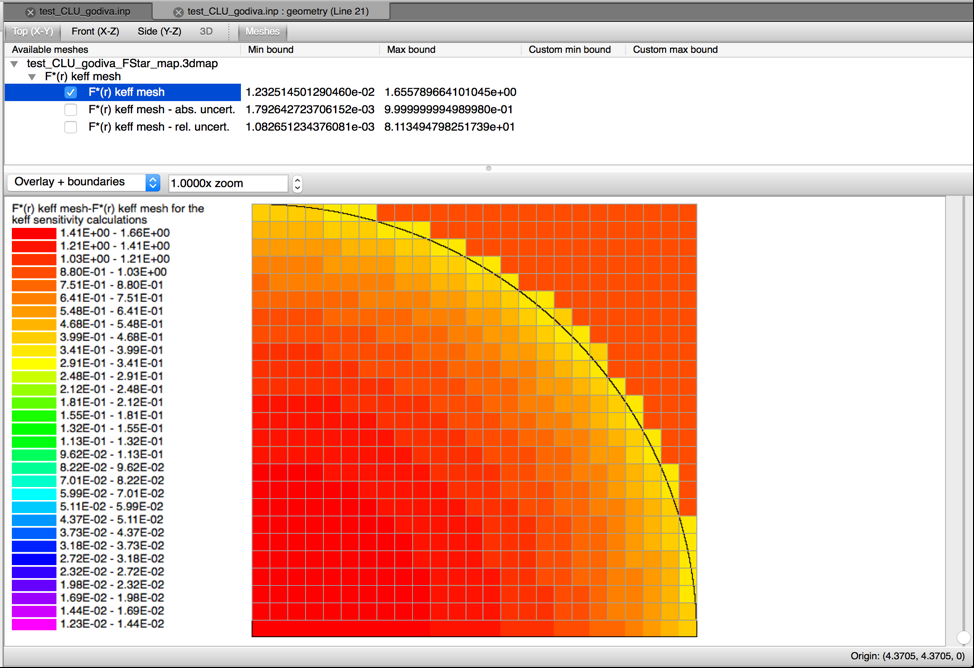
Fig. 6.2.4 \(F^{*}(r)\) mesh from a sample CLUTCH eigenvalue sensitivity calculation.
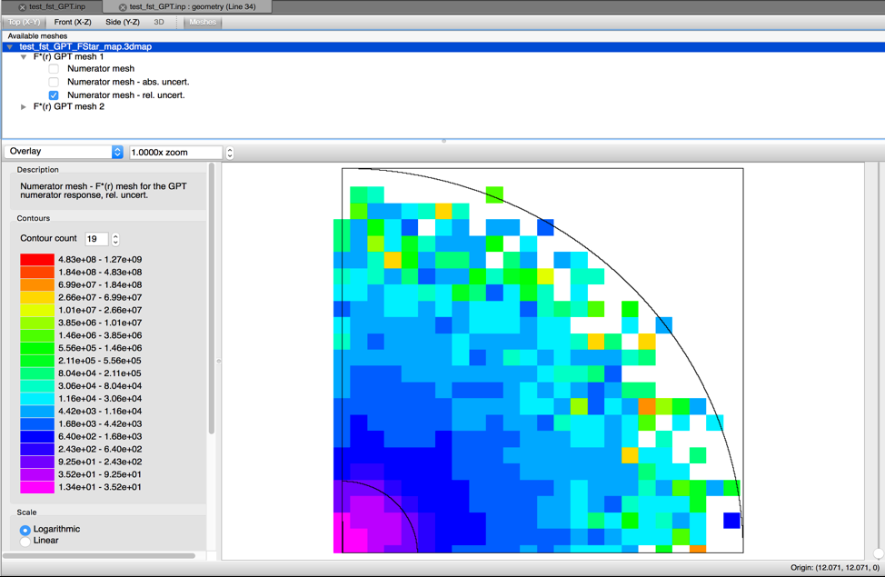
Fig. 6.2.5 \(F^{*}(r)\) meshes from a sample CLUTCH GPT sensitivity calculation.
Setting CET=7 will activate an experimental capability for detecting computational biases due to the undersampling of fission sites and particle histories during a Monte Carlo simulation. This capability does not calculate sensitivity coefficients and does not require selecting a number of latent generations or building an \(F^{*}\left( r \right)\) mesh. Instead, this approach scores flux and reaction rate tallies for various materials and nuclides in a system and reports the tallies to a .sdf file after the simulation ends, along with scores for various statistical metrics that may predict undersampling biases in the reported tallies. An undersampling metric calculation will produce four .sdf files, as described below:
Each of these undersampling metrics is described in detail in Reference [3d10]. The values reported in the _metric2/3/4.sdf files correspond to each of the tallies scored in the _metric1.sdf file. As in typical sensitivity coefficient .sdf files, the undersampling metric .sdfs report energy-dependent and energy-integrated information for various reaction rates in every material and nuclide in a system; however, the undersampling metric calculations also report information for flux tallies within each material/nuclide under the name of the fictitious isotope H-111. This undersampling metric capability is only peripherally related to the scope and application of sensitivity coefficient calculations and was included with CE TSUNAMI-3D predominantly to take advantage of the established TSUNAMI tally scoring framework and sensitivity visualization/postprocessing tools (i.e., Fulcrum).
Performing GPT sensitivity calculations with CE TSUNAMI requires the user to enter some additional input to specify the GPT response being examined in the calculation. For the IFP+CLUTCH GPT implementation (CET=5) users can define GPT reaction rate ratios using the “Definitions” and “SystemResponses” blocks (please see Sensitivity and uncertainty calculation data in the TSUNAMI-1D chapter), which are used similarly in TSUNAMI-1D. Both TSUNAMI-3D GPT capabilities can currently only accept total cross section (MT=1), fission (MT=18), n,gamma (MT=102), nu-fission (MT=452), or flux reaction response definitions. The CLUTCH-only GPT implementation (CET=4) currently cannot accept GPT response input from the Definitions and SystemResponses blocks, and may only calculate GPT sensitivity coefficients for one response per TSUNAMI-3D simulation. The input parameters for defining the GPT response in these (CET=4) calculations are described in Table 6.2.6. The two GEAR-MC implementations (CET=4 or CET=5) both require the user to specify a value for CFP; the CLUTCH-only GEAR-MC implementation requires the user to specify an \(F^{*}\left( r \right)\) mesh using the gridGeom block and the CGD parameter.

|
6.2.4.5. Sensitivity calculation data
A data block for controlling the sensitivity calculation is optional. If included, this data block begins with the keywords READ SAMS and ends with the keywords END SAMS. Any of the optional SAMS input data may be entered in free-form format between the READ SAMS and END SAMS keywords. The optional SAMS input data are shown with the default values specific to TSUNAMI-3D in Table 6.2.7. Certain options in Table 6.2.8 are not available for CE calculations. Parameters used to specify default covariance data to supplement or correct values on the files specified by coverx= are shown in Table 6.2.8. A more detailed explanation of the SAMS parameters is provided in the SAMS chapter.
Keyword |
Default value |
Description |
binsen |
F |
Produces SENPRO formatted binary sensitivity data file on unit 40 |
coverx= |
56groupcov7.1 |
Name of covariance data file to use for uncertainty analysis |
largeimp= |
100.0 |
Value for the absolute value of implicit sensitivities, which if exceeded, will be reset to 0.0 and print a warning message. |
makeimp* |
F |
Flag to cause implicit sensitivity coefficients to be generated. |
nocovar |
T |
Flag to cause uncertainty edit to be turned off (sets print_covar to F) |
nohtml |
F |
Flag to cause HTML output to not be produced. |
nomix |
F |
Flag to cause the sensitivities by mixture to be turned off |
pn=* |
3 |
Legendre order for moment calculations |
prtgeom* |
F |
Flag to cause the sensitivities to be output for each geometry region |
prtimp* |
F |
Prints explicit sensitivities coefficients, implicit sensitivity coefficients and complete sensitivity coefficients |
prtvols* |
F |
Flag to cause the volumes of the regions to be printed by SAMS |
useang* |
F |
Flag to cause the angular flux calculated in KENO to be used to calculate flux moments for sensitivity calculations. If angular fluxes were not computed by KENO, useang is set to false internally. |
usemom* |
T |
Flag to cause the flux moments calculated with KENO to be used to in sensitivity coefficient generation. If flux moments were not computed by KENO, usemom is set to false internally. |
unconstrainedchi |
F |
Flag to generate pre-SCALE 6 unconstrained chi (fission spectrum) sensitivities |
sensitivity_format= |
txt |
Specifies desired format for the resulting sensitivity data file (SDF). May be ‘txt’ for text-based format or ‘hdf5’ for HDF5-based format. |
*MG only |

|
Additionally, user-defined covariance data can be specified for individual nuclides and reactions using the COVARIANCE data block. This data block begins with the keywords READ COVARIANCE and ends with the keywords END COVARIANCE. Any of the optional COVARIANCE input data may be entered in free-form format between the READ COVARIANCE and END COVARIANCE keywords. The specifications for the COVARIANCE data block are described in the “User Input Covariance Data” section of the TSUNAMI-IP chapter of the TSUNAMI Utility Modules manual.
As the SAMS module generates HTML output, the optional HTML data block provides user control over some formats of the output. This data block begins with the keywords READ HTML and ends with the keywords END HTML. Any of the optional HTML input data may be entered in free-form format between the READ HTML and END HTML keywords. The specifications for the HTML data block are described in the “HTML Data” section or the TSUNAMI-IP chapter of the TSUNAMI Utility Modules manual.
6.2.4.6. Input termination
The input for TSUNAMI-3D must terminate with a line containing END in column 1. This END terminates the control sequence.
6.2.5. Sample problems
Five sample problems are given in this section. In each example, the use of a new feature is explained to guide the user in the proper definition of input models so that reliable sensitivity coefficients can be obtained. The user must ensure that the necessary options are employed for each model to obtain accurate results. Please note, the results shown here were generated with a previous version of SCALE, so current data libraries and code implementations may produce different results. However, the techniques demonstrated are applicable to the current version of TSUNAMI-3D.
6.2.5.1. Generating reference direct perturbation sensitivity coefficients
The accuracy of the energy-integrated sensitivity coefficients can be confirmed through the use of central difference direct perturbation sensitivity calculations. Through this technique, the sensitivity of keff to the number density of particular nuclide can be obtained. This sensitivity of keff to the number density is equivalent to the sensitivity of keff to the total cross section integrated over energy. Because the total cross section sensitivity coefficient tests much of the data used to compute all other sensitivity coefficients, it is considered an adequate test for verification. For each sensitivity coefficient examined by direct perturbation, the keff of the system is computed first with the nominal values of the input quantities, then with a selected nominal input value increased by a certain percentage, and then with the nominal value decreased by the same percentage. The direct perturbation sensitivity coefficient of keff to some input value \(\alpha\) is computed as
where \(\alpha^{+}\) and \(\alpha^{-}\) represent the increased and decreased values, respectively, of the input quantity \(\alpha\) and \(k_{\alpha^{+}}\) and \(k_{\alpha^{-}}\) represent the corresponding values of keff. In general, perturbations used for calculating direct perturbation sensitivities should be large enough to induce a statistically significant change (10 \(\sigma_{\text{keff}}\)) in the eigenvalue of the system but not large enough to induce second-order effects in the perturbed eigenvalue. Statistical uncertainties in the computed values of keff are propagated to uncertainties in direct perturbation sensitivity coefficients by standard error propagation techniques as
In MG TSUNAMI sensitivity calculations it is important to ensure that the keff value of the forward and adjoint solutions closely agree. If the keff values do not agree, then the quality of at least one of the transport calculations may be in question. Typically, the transport calculation of concern is the adjoint calculation. By default, TSUNAMI-3D triples the number of histories per generation requested for the forward case to produce the adjoint solution. Experience has shown that agreement to less than 0.5% difference in keff between the forward and adjoint calculations is adequate to obtain accurate sensitivity coefficients.
6.2.5.2. Simple MG Sample Problem
A simple sample problem with INFHOMMEDIUM MG cross section processing is based on an unreflected rectangular parallelepiped consisting of a homogeneous mixture UF4 and paraffin with an enrichment of 2 wt% in 235U. The H/235U atomic ratio is 294:1. The dimensions of the experiment are 56.22 \(\times\) 56.22 \(\times\) 122.47 cm [3d11]. For consistency with a TSUNAMI-1D model of the same sample problem, this experiment was modeled as a sphere with a critical radius of 38.50 cm. This configuration is used in the TSUNAMI-3D_K5-1 and TSUNAMI-3D_K6-1 sample problems distributed with SCALE. An annotated TSUNAMI-3D-K5 input for this experiment is shown in Fig. 6.2.6. The composition data are input as number densities for each nuclide. Because the material is treated as INFHOMMEDIUM, no explicit unit cell model is necessary, and the READ CELL block is omitted. The KENO V.a problem description contains parameter data to request 10,000 generations (gen=10000) with 3000 neutrons per generation (npg=3000), deactivate the HTML output for KENO V.a (htm=no), stop the forward calculation when keff has converged to one standard deviation of 0.005 (sig=0.005), and to stop the adjoint calculation when keff has converged to one standard deviation of 0.010 (asg=0.010). The KENO V.a geometry consists of nine concentric spheres, up to an outer radius of 38.5 cm, with each sphere containing the material defined as mixture 1. The geometry subdivision is necessary to adequately resolve the spatial dependence of the angular moments of the forward and adjoint flux solutions. The optional sensitivity calculation data block is used to request edits of the sensitivity coefficients for each region (prtgeom) and edits of the explicit, implicit, and complete sensitivity coefficients (prtimp). The code output from each functional module is not given here, but is described in the manual section for each functional module.
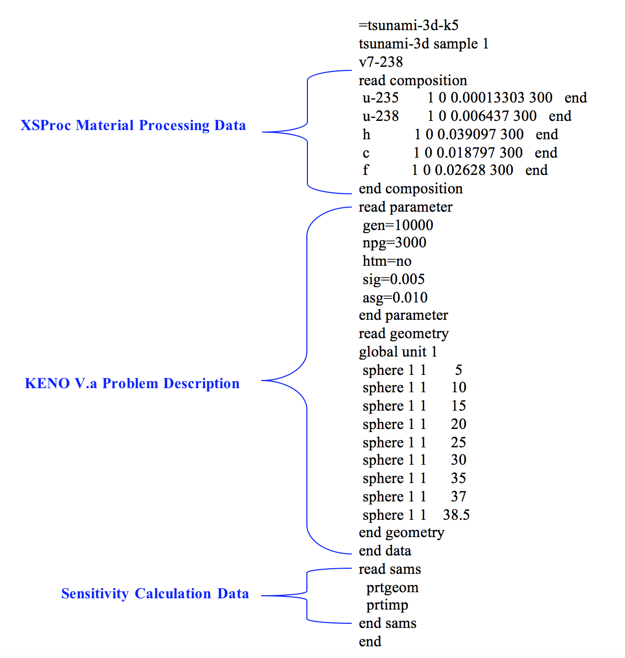
Fig. 6.2.6 TSUNAMI-3D-K5 simple sample problem input.
For this problem, direct perturbation results were obtained for the number densities of each nuclide using an equivalent 1D model. In these calculations, the number density of each nuclide was perturbed by \(\pm\) to the number density is equivalent to the sensitivity of keff to the total cross section, integrated over energy. The direct perturbation sensitivity coefficients were computed by using the keff values from the unperturbed and perturbed cases in Eq. (6.2.27).
This experiment was modeled with the nine-region model shown in Fig. 6.2.6, and as a single computational region (not shown). Flux moments were expanded to third order in both cases, which is the default configuration. TSUNAMI-3D-K5 automatically increases the number of particles per generation by a factor of three for the adjoint analysis. For the single region case, the keff values for the forward and adjoint cases are in good agreement at 1.00682 +/- 0.00094, and 1.0013 +/- 0.0049, respectively. The sensitivity results shown in Table 6.2.9 were extracted from the output file from the edit titled “Energy, Region, and Mixture Integrated Sensitivity Coefficients for this Problem.” The uncertainty in the sensitivity coefficients represents one standard deviation and is present due to the use of Monte Carlo methods to compute the fluxes and keff. These results indicate similarity with the direct perturbation results for some nuclides but not for others. Differences between the TSUNAMI-3D-K5 results and the direct perturbation results vary 1% for 238U up to 16% for 1H. The results from the TSUNAMI-3D-K5 analysis with the model divided into nine spherical shells, with all other parameters held constant, are also shown in Table 6.2.9. These results compare much more favorably with the direct perturbation results. For this model, all TSUNAMI-3D-K5 sensitivities agree with the direct perturbation values within 0.1% for 1H up to a maximum difference of 1.5% for 238U.
The differences in the results from the two TSUNAMI-3D models, one region and nine regions, are due to the summation of the product of the forward and adjoint fluxes over the regions in the problem. For a region in which the flux moments vary greatly by position, subdividing the geometry will provide better resolution of the variation of the flux across the system and will produce more accurate results. The number of regions necessary for accurate computation of the sensitivity coefficients was determined through an iterative process. Models divided into more regions produce the equivalent results to those produced by the nine-region model. Increasing the number of computational regions increases the run time for this problem by about 10%.
The sensitivity results from the nine-region model using TSUNAMI-3D-K5 with PARM=CENTRM, which does not include the contributions from the implicit sensitivity coefficients, are also shown in Table 6.2.9. The differences between the TSUNAMI-3D-K5 PARM=CENTRM and the direct perturbation results are 16% for 1H and 19% for 238U. The use of the default cross section processing with the sensitivity versions of the resonance processing codes is strongly recommended. However, TSUNAMI-3D-K5 with PARM=CENTRM should produce accurate results for fast systems where resonance self-shielding is not important. This is illustrated with the second sample problem for TSUNAMI-1D and will not be repeated here.

|

|
The uncertainty information from SAMS for the UF4 sample problem is shown in Example 6.2.1. Based on the 44GROUPCOV covariance data file, the uncertainty in \(k_{eff}\) due to these covariance data is 0.6110% \(\Delta k/k\). A more detailed description of the uncertainty information is given in the SAMS chapter.
The energy-dependent sensitivity data are available in the sensitivity
data file, which is returned to the same directory as the input file and
given the same name as the user’s input file with the extension .sdf.
In the case of the nine-region model, the sensitivity data file contains
495 individual sensitivity profiles with varying reaction types, each in
the 238-group energy structure. There are 45 profiles that are
integrated over all regions, one for each reaction of each nuclide in
the system. The sum of the sensitivity coefficients for the same nuclide
in all mixtures is printed unless nomix is entered in the SAMS data
block, so there are an additional 45 profiles, one for each reaction of
each nuclide in mixture 1. Additionally, because prtgeom was entered
in the SAMS data block, each reaction of each nuclide for each region in
the system model is represented with a sensitivity profile. There are
nine regions in the model, each with 45 sensitivity profiles, making for
a total of 495 sensitivity profiles on the data file and a total of
117,810 energy-dependent sensitivity coefficients.
Some plots of the energy-dependent sensitivity data from the nine-region model of the sample problem were generated with the plotting capabilities of Fulcrum. Energy-dependent sensitivity profiles for 235U fission and 1H elastic scattering are shown in Fig. 6.2.7. The error bars represent one standard deviation for the statistical uncertainty due to the use of Monte Carlo methods to compute the fluxes and \(k_{eff}\).
-----------------------------
  Uncertainty Information
-----------------------------


the relative standard deviation of k-eff (% delta-k/k)
due to cross-section covariance data is:

  0.6110 +/- 0.0000 % delta-k/k

 contributions to uncertainty in k-eff (% delta-k/k) by
 individual energy covariance matrices:

 covariance matrix

        nuclide-reaction        with        nuclide-reaction            % delta-k/k due to this matrix
 ------------------------------      -------------------------------  -----------------------------------
         u-238 n,gamma                       u-238 n,gamma                 3.8714E-01 +/- 6.2871E-06
         u-235 nubar                         u-235 nubar                   2.8509E-01 +/- 7.9001E-06
         u-238 n,n'                          u-238 n,n'                    2.2073E-01 +/- 7.7594E-06
         u-235 n,gamma                       u-235 n,gamma                 1.6006E-01 +/- 1.7559E-06
          f-19 elastic                        f-19 elastic                 1.3624E-01 +/- 5.0707E-06
         u-238 elastic                       u-238 n,n'                   -1.2828E-01 +/- 1.7674E-06
         u-235 fission                       u-235 n,gamma                 1.2387E-01 +/- 8.3076E-07
         u-235 fission                       u-235 fission                 1.2134E-01 +/- 1.2085E-06
           h-1 elastic                         h-1 elastic                 1.1972E-01 +/- 2.1606E-06
          f-19 elastic                        f-19 n,n'                   -1.1793E-01 +/- 3.1965E-06
          f-19 n,n'                           f-19 n,n'                    1.1286E-01 +/- 3.8652E-06
         u-235 chi                           u-235 chi                     8.8178E-02 +/- 1.5583E-05
         u-238 elastic                       u-238 elastic                 6.9520E-02 +/- 1.1586E-06
         u-238 nubar                         u-238 nubar                   5.8614E-02 +/- 5.4192E-07
           h-1 n,gamma                         h-1 n,gamma                 5.0829E-02 +/- 1.6728E-07
         u-238 elastic                       u-238 n,gamma                 5.0286E-02 +/- 1.7408E-06
          f-19 n,alpha                        f-19 n,alpha                 1.9795E-02 +/- 1.0127E-07
         u-238 fission                       u-238 fission                 1.7394E-02 +/- 3.4394E-08
             c elastic                           c elastic                 1.5520E-02 +/- 5.5754E-08
         u-238 n,2n                          u-238 n,2n                    1.3981E-02 +/- 1.2056E-07
          f-19 n,gamma                        f-19 n,gamma                 9.7994E-03 +/- 6.0845E-09
             c n,n'                              c elastic                -9.0325E-03 +/- 3.2330E-08
             c n,n'                              c n,n'                    8.6479E-03 +/- 5.6289E-08
          f-19 elastic                        f-19 n,alpha                 6.6750E-03 +/- 1.2243E-08
         u-238 chi                           u-238 chi                     5.8854E-03 +/- 6.7274E-08
         u-235 elastic                       u-235 n,gamma                 4.4783E-03 +/- 8.4753E-09
         u-235 elastic                       u-235 fission                -3.3039E-03 +/- 1.0089E-08
         u-238 fission                       u-238 n,gamma                 2.7661E-03 +/- 8.1090E-10
          f-19 n,p                            f-19 n,p                     2.0897E-03 +/- 1.3810E-09
         u-238 elastic                       u-238 n,2n                   -1.9405E-03 +/- 1.8719E-09
         u-238 elastic                       u-238 fission                -1.8278E-03 +/- 3.9798E-10
             c n,alpha                           c n,alpha                 1.6271E-03 +/- 1.2097E-09
             c n,gamma                           c n,gamma                 1.4922E-03 +/- 1.4387E-10
         u-235 n,n'                          u-235 n,n'                    1.3833E-03 +/- 2.5316E-10
         u-235 elastic                       u-235 n,n'                   -8.8072E-04 +/- 6.2537E-11
          f-19 elastic                        f-19 n,p                     5.9136E-04 +/- 2.5027E-10
          f-19 elastic                        f-19 n,gamma                 4.4592E-04 +/- 4.9929E-10
         u-235 elastic                       u-235 elastic                 4.3974E-04 +/- 3.1277E-11
          f-19 n,d                            f-19 n,d                     2.7814E-04 +/- 4.7485E-11
         u-235 n,2n                          u-235 n,2n                    1.5578E-04 +/- 1.1389E-11
             c n,n'                              c n,alpha                -1.2708E-04 +/- 7.1578E-10
          f-19 elastic                        f-19 n,2n                   -6.9247E-05 +/- 1.2530E-11
          f-19 elastic                        f-19 n,d                     6.6212E-05 +/- 1.0124E-11
          f-19 n,t                            f-19 n,t                     6.3390E-05 +/- 3.8183E-12
         u-235 elastic                       u-235 n,2n                   -2.7965E-05 +/- 3.3228E-13
          f-19 n,2n                           f-19 n,2n                    2.1907E-05 +/- 1.0175E-12
          f-19 n,n'                           f-19 n,2n                   -1.9896E-05 +/- 5.7304E-12
          f-19 elastic                        f-19 n,t                     1.4406E-05 +/- 5.0542E-13
             c n,n'                              c n,gamma                 7.0412E-06 +/- 1.1010E-14
             c n,d                               c n,d                     6.9094E-07 +/- 9.1360E-15
             c n,p                               c n,p                     3.8587E-07 +/- 2.0164E-15
             c n,n'                              c n,d                    -2.8704E-07 +/- 0.0000E+00
             c n,n'                              c n,p                    -1.4206E-07 +/- 0.0000E+00

 Note: relative standard deviation in k-eff can be computed from
 individual values by adding the square of the values with positive signs and
 subtracting the square of the values with negative signs, then taking the square root
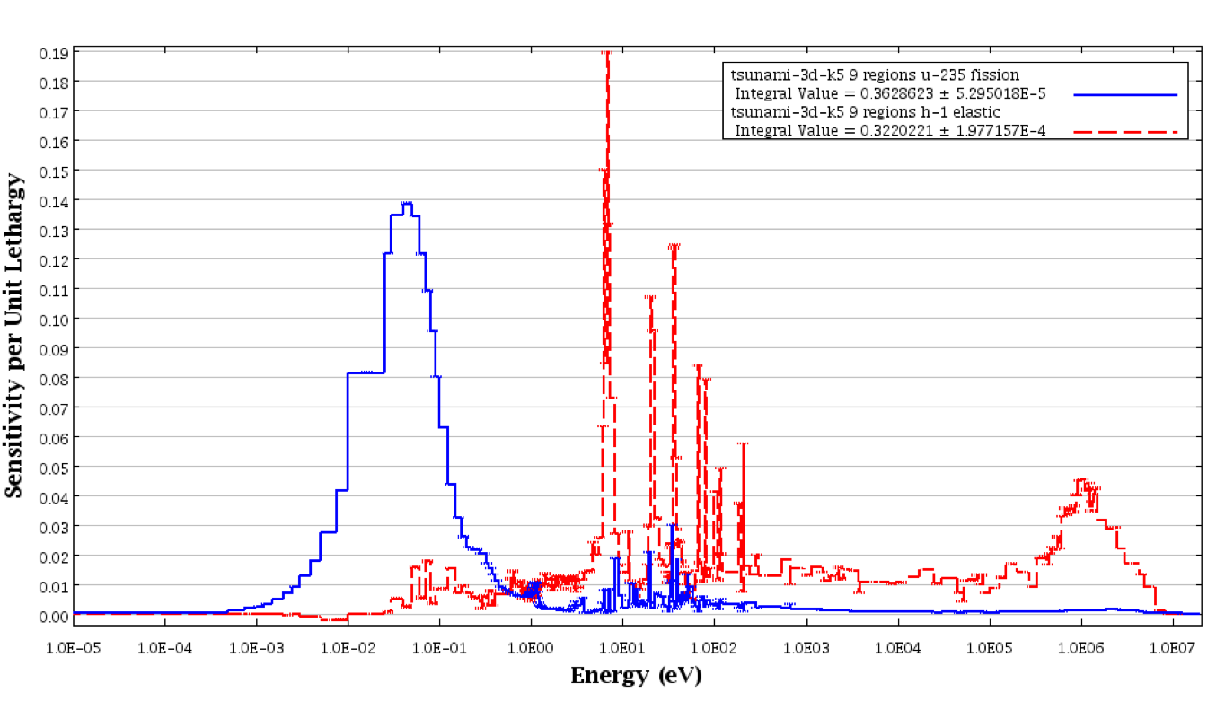
Fig. 6.2.7 Energy-dependent sensitivity profiles from TSUNAMI-3D-K5 for simple sample problem.
6.2.5.2.1. Multigroup sample problem with spatial flux mesh
In the previous example, subdivision of the system geometry was necessary to obtain adequate resolution of the flux solution to obtain the appropriate product of the forward and adjoint fluxes necessary for the sensitivity calculations. To simplify the geometry refinement procedure, the meshing of KENO V.a or KENO-VI is used where fluxes are tallied in a cubic mesh that is superimposed over each region of the system geometry. If mesh fluxes are generated in the KENO solution, they are automatically used by the SAMS module in the calculation of the sensitivity coefficients.
To demonstrate the use of the mesh flux option in TSUNAMI-3D-K5, another simple system has been selected. This system is an unreflected rectangular parallelepiped consisting of a homogeneous mixture of UF4 and paraffin with an enrichment of 2 wt% in 235U. The H/235U atomic ratio is 972:1. The dimensions of the experiment are 81.45 \(\times\) 86.70 \(\times\) 88.22 cm. This system is identified as LEU-COMP-THERM-033 case 45 from the International Handbook of Evaluated Criticality Safety Benchmark Experiments (IHECSBE). [3d11] The model provided in the IHECSBE was converted to a TSUNAMI-3D-K5 input and is shown in Example 6.2.2. Here the experiment is modeled as a single cuboid. This model is included as an example and is not distributed as a TSUNAMI-3D sample problem.
Direct perturbation sensitivity results were obtained for 235U, 238U, and 1H with a \(\pm\) value converged to a standard deviation of 0.0001 (sig=0.0001). For the model shown in Example 6.2.2, the forward and adjoint keff values agreed well at 0.99250 \(\pm\) 0.00056 and 0.9905 \(\pm\) 0.0049, respectively. The direct perturbation results and the TSUNAMI-3D-K5 results are shown in Table 6.2.11. When modeled as a single region, the TSUNAMI-3D-K5 results differed from the direct perturbation results by 2.6% for 238U, 3.1% for 235U, and 15% for 1H.
To improve the agreement in the values, the model was divided into 6 cuboids nested inside of each other. The input for this model is given in Example 6.2.3 and is illustrated in Fig. 6.2.8. The results for this model are also given in Table 6.2.10. Here the TSUNAMI-3D-K5 sensitivity coefficients agree with the direct perturbation within 0.3% for 238U, 1.7% for 235U, and 0.8% for 1H.
To simplify the generation of a refined geometrical representation of this system, the same geometry as the initial model was used with an 8 cm mesh for the flux tallies. The input for this model is shown in Example 6.2.4. The mesh is illustrated in Fig. 6.2.9, using a larger (15 cm) mesh interval for illustrative purposes. The mesh flux option is activated by entering mfx=yes in the input, and the size of the mesh is defined with the msh=8 entry. The 8 following msh= indicates that a cubic grid with a length of 8 cm on the side of each cube will be superimposed on each geometry region. For this system, the flux will be tallied in 1728 mesh intervals. When the forward and adjoint mesh flux solutions are processed by the SAMS module, the product of the forward and adjoint solutions are produced for each mesh interval, then summed for each region. This technique provides a simple input parameter to produce accurate sensitivity coefficients. The results from TSUNAMI-3D-K5 with an 8 cm mesh flux are given in Table 6.2.11. Similar to the results with the manual subdivision, sensitivity coefficients agree with the direct perturbation within 0.7% for 238U, 2.1% for 235U, and 0.03% for 1H.
The sensitivity results for 235U and 238U show little variation with modifications in the geometry subdivision. The products of the forward and adjoint flux moments, which are derived from the angular flux solution, are most impacted by the mesh flux. The flux moments are used to compute the scattering terms of the sensitivity coefficients. For isotopes with limited scattering cross sections, such as 235U and 238U, the impact of refinement of the flux solution is reduced.
=tsunami-3d-k5
uf4 paraffin mixture u2f4-6
v6-238
read composition
 h-poly      6 0 0.060586 300   end
 f           6 0 0.012302 300   end
 c           6 0 0.029128 300   end
 u-235       6 0 6.2282e-05 300   end
 u-238       6 0 0.0030126 300   end
 u-234       6 0 6.2548e-07 300   end
end composition
read parameter
 gen=10000
 npg=10000
 sig=0.0001
end parameter
read geometry
global unit 1
 cuboid 6 1   40.725  -40.725    43.35   -43.35    44.11   -44.11
end geometry
end data
read sams
  prtgeom prtimp
end sams
end

|
=tsunami-3d-k5
uf4 paraffin mixture u2f4-6
v6-238
read composition
 h-poly      6 0 0.060586 300   end
 f           6 0 0.012302 300   end
 c           6 0 0.029128 300   end
 u-235       6 0 6.2282e-05 300   end
 u-238       6 0 0.0030126 300   end
 u-234       6 0 6.2548e-07 300   end
end composition
read parameter
 gen=10000
 npg=10000
 sig=0.0001
end parameter
read geometry
global unit 1
 cuboid 6 1       10      -10       10      -10       10      -10
 cuboid 6 1       20      -20       20      -20       20      -20
 cuboid 6 1       30      -30       30      -30       30      -30
 cuboid 6 1       35      -35       35      -35       35      -35
 cuboid 6 1       38      -38       41      -41       42      -42
 cuboid 6 1   40.725  -40.725    43.35   -43.35    44.11   -44.11
end geometry
end data
read sams
  prtgeom prtimp
end sams
end
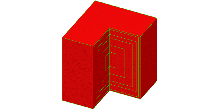
Fig. 6.2.8 Cutaway view of LEU-COMP-THERM-033 case 45 with manual subdivision.
=tsunami-3d-k5
uf4 paraffin mixture u2f4-6
v6-238
read composition
 h-poly      6 0 0.060586 300   end
 f           6 0 0.012302 300   end
 c           6 0 0.029128 300   end
 u-235       6 0 6.2282e-05 300   end
 u-238       6 0 0.0030126 300   end
 u-234       6 0 6.2548e-07 300   end
end composition
read parameter
 gen=10000
 npg=10000
 sig=0.0001
 mfx=yes
 msh=8
end parameter
read geometry
global unit 1
 cuboid 6 1   40.725  -40.725    43.35   -43.35    44.11   -44.11
end geometry
end data
read sams
 prtimp prtgeom
end sams
end
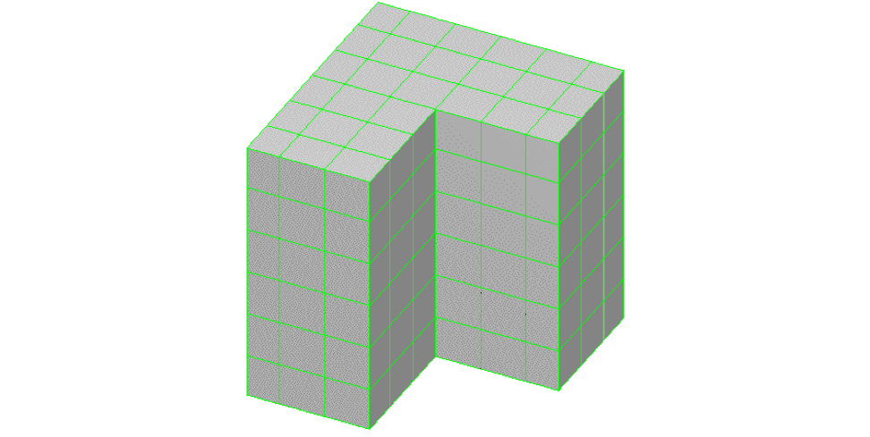
Fig. 6.2.9 TSUNAMI-3D-K5 input for LEU-COMP-THERM-033 case 45 with 8 cm automated mesh.
6.2.5.3. Complex sample problem
A more complex sample problem is a critical assembly of 4.31 wt%-enriched UO2 fuel rods with a pitch of 2.54 cm in clusters that are separated by copper plates. This system is identified as LEU-COMP-THERM-009 case 10 from the IHECSBE. This system is used for sample problem TSUNAMI-3D_K5-2 that is distributed with SCALE. The TSUNAMI-3D_K5-2 sample problem input is shown in Example 6.2.5, and the geometry is illustrated in Fig. 6.2.10. The KENO V.a input section for this model is essentially the same as that presented in the IHECSBE except that the parameter data have been modified for the TSUNAMI calculation. Also, in the IHECSBE model, all water was assigned to the same mixture. For this model, the water in the reflector region is entered as a separate mixture from the water in the pin cell to generate separate sensitivity coefficients in these regions.
For this system, direct perturbation results were obtained for 235U, 238U, and 1H in the pin cell model (mixture 2) and for 1H in the reflector (mixture 7). Direct perturbation sensitivity coefficients can be difficult to obtain for large systems using Monte Carlo techniques. For a small change in a number density (1% or 2%), the effect of keff may not be significant enough to be observed outside of statistical uncertainties. If a larger perturbation (5% or 10%) is used, the effect on keff may not be linear and may produce misleading results. Also, if the magnitude of the difference in keff between the baseline value and the increased density perturbed model is different from the magnitude of the difference in keff between the baseline model and the decreased density perturbed model, the response may be nonlinear. In these calculations, the amount of the perturbation was carefully chosen to produce approximately 10 standard deviations of change in keff between the perturbed and unperturbed case. The amount of perturbation for each nuclide is shown in Table 6.2.12.
TSUNAMI-3D-K5 was executed with no flux mesh, a 15 cm flux mesh, and a 5 cm flux mesh using the default coordinate transform setting (tfm=yes). Also, the 15 cm and 5 cm mesh cases were run with the coordinate transform turned off (tfm=no).
Where a region is repeatedly used in KENO, the flux data are averaged over all occurrences of a region. In this model, only one fuel pin is explicitly modeled. This single pin is used repeatedly in arrays to create the system model. The flux data for this single pin are averaged over all occurrences throughout the system to create the sensitivity data. Using the mesh flux option, the flux is accumulated for the fuel pin in each mesh interval. For the model with no mesh, the flux in the UO2 portion of the fuel pin is averaged over a single region. With the 15 cm mesh, the flux in UO2 is accumulated in 126 separate mesh intervals distributed across the core. For the 5 cm mesh, the flux in UO2 is accumulated in 2280 mesh intervals. For all regions of the model with no mesh, the flux is only stored for 17 unique locations, one for each region. For the 15 cm mesh, the flux is stored in 1968 unique mesh intervals. For the 5 cm mesh mode, the flux is stored in 34,298 unique mesh intervals.
=tsunami-3d-k5
tsunami-3d sample 2
v7-238
read composition
 u-234       1 0 5.1835e-06 295   end
 u-235       1 0 0.0010102 295   end
 u-236       1 0 5.1395e-06 295   end
 u-238       1 0 0.022157 295   end
 o           1 0 0.046753 295   end
 h           2 0 0.066675 295   end
 o           2 0 0.033338 295   end
 al          3 0 0.058433 295   end
 cr          3 0 6.231e-05 295   end
 cu          3 0 6.3731e-05 295   end
 mg          3 0 0.00066651 295   end
 mn          3 0 2.2115e-05 295   end
 ti          3 0 2.5375e-05 295   end
 cu          3 0 3.0967e-05 295   end
 si          3 0 0.00034607 295   end
 fe          3 0 0.00010152 295   end
 c           4 0 0.043562 295   end
 h           4 0 0.058178 295   end
 ca          4 0 0.002566 295   end
 s           4 0 0.0004782 295   end
 si          4 0 9.636e-05 295   end
 o           4 0 0.012461 295   end
 h           5 0 0.056642 295   end
 c           5 0 0.035648 295   end
 o           5 0 0.014273 295   end
 c           6 0 0.0015194 295   end
 cu          6 0 0.084128 295   end
 fe          6 0 3.8444e-06 295   end
 mg          6 0 4.4168e-06 295   end
 na          6 0 4.6695e-06 295   end
 o           6 0 0.00010064 295   end
 si          6 0 3.8223e-05 295   end
 s           6 0 3.3474e-06 295   end
 h           7 0 0.066675 295   end
 o           7 0 0.033338 295   end
end composition
read celldata
  latticecell squarepitch fuelr=0.6325 1 gapr=0.6415 0 cladr=0.7075 3 hpitch=1.27 2 end
  inf 4 end
  inf 5 end
  inf 6 end
  inf 7 end
end celldata
read parameter
 npg=10000
 gen=10000
 sig=0.0002
 tfm=yes
 msh=15
end parameter
read geometry
unit 1
com='fuel pin '
 zcylinder 1 1  0.6325   92.075        0
 zcylinder 0 1  0.6415   92.075        0
 zcylinder 4 1  0.6415  94.2975  -2.2225
 zcylinder 3 1  0.7075  94.2975  -2.2225
 cuboid 2 1     1.27    -1.27     1.27    -1.27  94.2975  -2.2225

Figure 6.2.14. TSUNAMI-3D LEU-COMP-THERM-009 case 10 sample problem input.

unit 2
com='array of fuel pins '
  array 1       0        0  -2.2225
 replicate 5 1       0        0        0        0        0     2.54 1
 replicate 7 1       0        0     7.64     7.64        0        0 1
unit 3
com='water between clusters 7.422 cm '
 cuboid 7 1    7.422        0    27.96    -7.64  94.2975  -2.2225
 cuboid 5 1    7.422        0    27.96    -7.64  94.2975  -4.7625
unit 4
com='cu poison plate between clusters,0.646 cm wide '
 cuboid 6 1    0.646        0    27.96    -7.64     91.5        0
 cuboid 7 1    0.646        0    27.96    -7.64  94.2975  -2.2225
 cuboid 5 1    0.646        0    27.96    -7.64  94.2975  -4.7625
unit 5
com='water between clusters,0.084cm wide '
 cuboid 7 1    0.084        0    27.96    -7.64  94.2975  -2.2225
 cuboid 5 1    0.084        0    27.96    -7.64  94.2975  -4.7625
global unit 6
com='clusters with water between '
  array 2       0        0  -2.2225
 replicate 7 1    30.5     30.5    22.86    22.86  12.7775     15.3 1
end geometry
read array
ara=1 nux=15 nuy=8 nuz=1
 fill
    1    1    1    1    1    1    1    1    1    1    1    1    1    1    1
    1    1    1    1    1    1    1    1    1    1    1    1    1    1    1
    1    1    1    1    1    1    1    1    1    1    1    1    1    1    1
    1    1    1    1    1    1    1    1    1    1    1    1    1    1    1
    1    1    1    1    1    1    1    1    1    1    1    1    1    1    1
    1    1    1    1    1    1    1    1    1    1    1    1    1    1    1
    1    1    1    1    1    1    1    1    1    1    1    1    1    1    1
    1    1    1    1    1    1    1    1    1    1    1    1    1    1    1
 end fill
ara=2 nux=9 nuy=1 nuz=1
 fill
    2    3    4    5    2    5    4    3    2
 end fill
end array
end data
read sams
  prtgeom
  prtimp
end sams
end
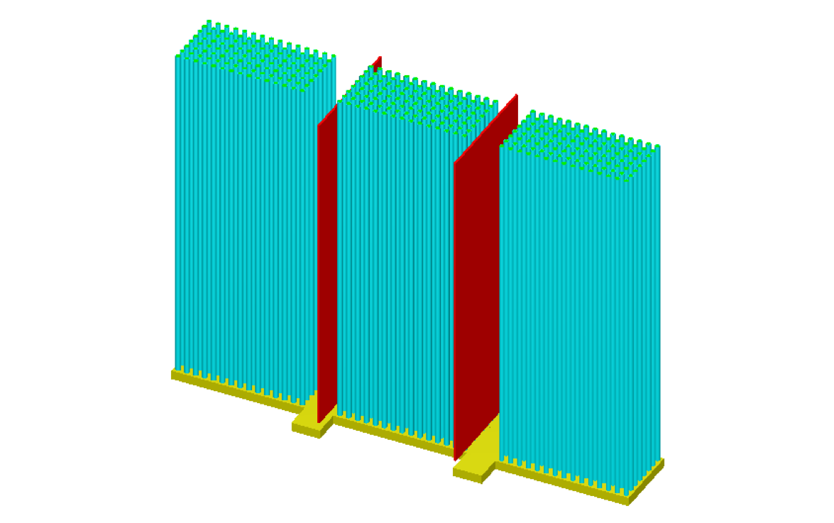
Fig. 6.2.10 Graphical representation of KENO V.a geometry for LEU-COMP-THERM-009 case 10 sample problem.
Sensitivity coefficients and their statistical uncertainties are shown in Table 6.2.12. For 235U, the TSUNAMI-3D and direct perturbation results agree within one standard deviation for all cases. For 238U, TSUNAMI-3D agrees within two standard deviations for all cases except the no-mesh case, which disagrees by more than four standard deviations. Similarly for 1H in the pin cell, all meshed cases agree with the direct perturbation results to less than one standard deviation, but the case with no geometrical subdivision disagrees by five standard deviations. For 1H in the reflector, again, the meshed cases all agree well with the direct perturbation results, but the non-mesh case shows large discrepancy of 21 standard deviations.
Also, only small differences are observed with and without the transform where an adequate flux mesh is used. Because of the computational resources required for computing the transform while performing neutron tracking, setting tfm=no can decrease runtime by ~50%. However, in cases where an adequate computational mesh is not used, setting tfm=no can lead to erroneous results.
The energy-dependent sensitivity profiles for 1H elastic scattering for the three TSUNAMI-3D models are shown in Fig. 6.2.11. The differences in the groupwise sensitivity coefficients are most pronounced in the intermediate- to high-energy regions.

|
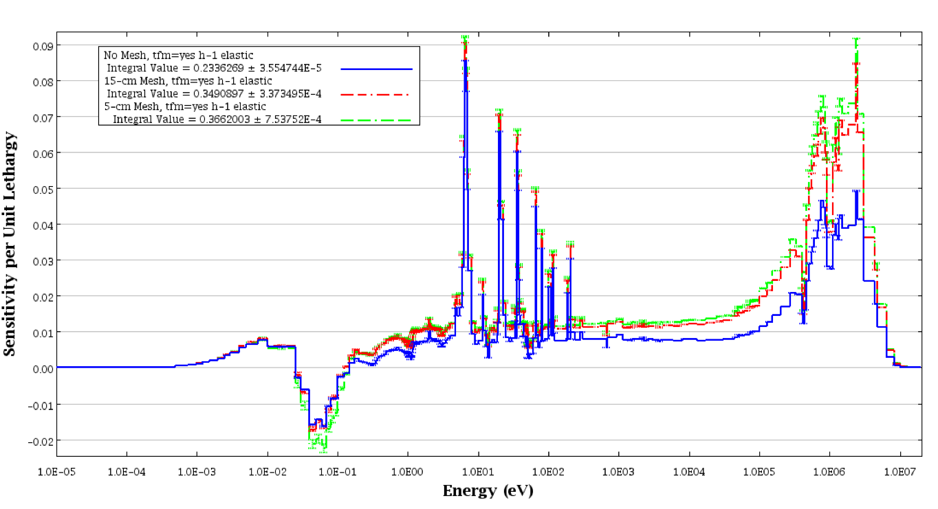
Fig. 6.2.11 Sensitivity profiles from TSUNAMI-3D for 1H elastic scattering in mixture 2 of LEU-COMP-THERM-009 case 10 sample problem.
6.2.5.3.1. Loosely coupled sample problem
Another sample problem demonstrates the use of the GRID input block to input a nonuniform mesh. This sample problem consists of three tanks containing plutonium nitrate solution that are suspended in air inside of a large concrete room. This system is identified as PU-SOL-THERM-014 case 19 in the IHECSBE. A TSUNAMI-3D-K5 input for this system is shown in Example 6.2.6. The system geometry is illustrated in Fig. 6.2.12, where the concrete room is shown in light blue and the solution tanks are shown in dark blue. A single tank is shown in Fig. 6.2.13, where the tank wall is shown in dark blue and the plutonium nitrate solution is shown in gray.
The KENO V.a option to compute the matrix keff by hole was used (mkh=yes) to give the self-multiplication of each tank. This analysis revealed a system keff of 1.0049 \(\pm\) 0.0003 for the forward case and 1.002 \(\pm\) 0.002 for the adjoint case. The keff of a single tank for the forward solution was found to be 1.0044 \(\pm\) 0.0017. Thus the interaction between the tanks has a limited effect on the system multiplication factor.
Direct perturbation sensitivity coefficients were generated for 239Pu, 240Pu, and 1H in the solution using number density perturbations to produce a 20 standard deviation change in keff, where the requested keff convergence for the CSAS direct perturbation calculation was 10-4. These values are shown in Table 6.2.13 along with the corresponding TSUNAMI-3D results. The results generated by the model shown in Example 6.2.6, which has no geometric subdivision, agree well with the direct perturbation results for 239Pu, but the 1H values differ by more than six standard deviations, indicating poor agreement.
=tsunami-3d-k5
PU-SOL-THERM-014-019
v7-238
read comp
PU-238 1 0 2.0965E-8 300.0 END
PU-239 1 0 2.7672E-4 300.0 END
PU-240 1 0 1.2209E-5 300.0 END
PU-241 1 0 9.0317E-7 300.0 END
PU-242 1 0 4.5817E-8 300.0 END
AM-241 1 0 1.1013E-7 300.0 END
N      1 0 2.3837E-3 300.0 END
O      1 0 3.7011E-2 300.0 END
H      1 0 6.0930E-2 300.0 END
FE     1 0 2.5125E-6 300.0 END
CA     1 0 1.3839E-6 300.0 END
CR     1 0 6.6711E-7 300.0 END
NI     1 0 5.3151E-7 300.0 END
FE     2 0 5.8686E-2 300.0 END
CR     2 0 1.6469E-2 300.0 END
NI     2 0 8.1061E-3 300.0 END
MN     2 0 1.7319E-3 300.0 END
SI     2 0 1.6939E-3 300.0 END
C      2 0 1.5857E-4 300.0 END
P      2 0 6.1439E-5 300.0 END
S      2 0 4.4518E-5 300.0 END
H      3 0 1.0350E-2 300.0 END
B-10   3 0 1.6020E-6 300.0 END
O      3 0 4.3470E-2 300.0 END
AL     3 0 1.5630E-3 300.0 END
SI     3 0 1.4170E-2 300.0 END
CA     3 0 6.4240E-3 300.0 END
FE     3 0 7.6210E-4 300.0 END
END COMP
READ PARA
TME=500.0 GEN=15000 NPG=5000  NSK=5 TBA=10.0
RUN=YES AMX=NO FLX=NO FDN=NO FAR=NO PLT=NO sig=0.0001
END PARA
READ GEOM
UNIT 1
COM='CYLINDER + SOLUTION'
CYLINDER 1 1 14.7 -10.7555 -50.5855
CYLINDER 0 1 14.7 50.5855 -50.5855
CYLINDER 2 1 15.0 51.7855 -51.9145
GLOBAL
UNIT 2
COM='CONCRETE BUILDING + ARRAY'
CUBOID 0 1 2P605.0 2P440.0 2P500.0
HOLE 1   -310.0      55.0        -344.0855
HOLE 1   -160.0   -95.0        -344.0855
HOLE 1   -310.0   -95.0        -344.0855
CUBOID 3 1 2P750.0 2P585.0 570.0 -540.0
END GEOM
READ STAR
NST=1
END STAR
END DATA
end
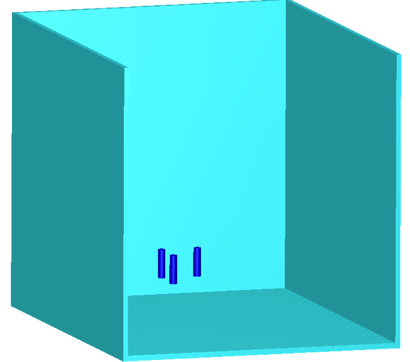
Fig. 6.2.12 Cutaway view of PU-SOL-THERM-014 case 19 sample problem.
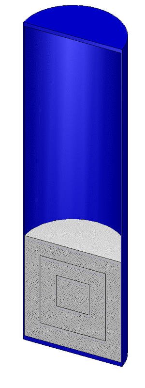
Fig. 6.2.13 Cutaway view of single solution tank from PU-SOL-THERM-014 case 19 sample problem.
1H |
239Pu |
|
|---|---|---|
Percent change in number density for direct perturbation |
0.32 |
2.39 |
Direct perturbation |
5.99E-01 \(\pm\) 2.56E-02 |
7.57E-02 \(\pm\) 8.29E-03 |
TSUNAMI-3D-K5 base model |
4.34E-01 \(\pm\) 1.82E-05 |
7.58E-02 \(\pm\) 4.42E-06 |
TSUNAMI-3D-K5 grid geometry model |
6.05E-01 \(\pm\) 3.42E-04 |
7.84E-02 \(\pm\) 3.80E-05 |
Because of the large size of the room included in this model relative to the size of the fuel tanks, use of the uniform mesh flux proved to be impractical due to excessive memory requirements. The directional dependence of the flux needs to be computed separately for each tank through the use of adequate spatial refinement with the flux mesh through the use of the grid geometry input.
The GRID block in KENO V.a and KENO-VI enables the use of a nonuniform mesh for this problem that is coarse throughout the room to save memory, yet refined within the fueled regions to obtain accurate results. As with previous examples, the use of a sufficiently fine mesh provides accurate results without the use of the transform (tfm=no). The TSUNAMI-3D-K5 input listing for this model using the user-defined GRID is shown in Example 6.2.7, where the transform is disabled with tfm=no, the mesh fluxes are requested with mfx=yes, and the grid is defined in the read grid block. The msh parameter that defines a uniform mesh is not used. The input requirements for the grid are described in the READ GRID section of the KENO documentation and will not be repeated here. It is required that the user-defined mesh completely encloses the geometry of the system. In the model in Example 6.2.11, the grid extends past the geometry by 1 cm in each direction to ensure that potential round-off errors do not cause the grid to appear to terminate inside the geometry at any point.
When the user-defined grid is used without the transform, the TSUNAMI-3D-K5 and direct perturbation sensitivities agree within one standard deviation for both 1H and 239Pu, as shown in Table 6.2.13.
=tsunami-3d-k5
PU-SOL-THERM-014-019
v7-238
read comp
PU-238 1 0 2.0965E-8 300.0 END
PU-239 1 0 2.7672E-4 300.0 END
PU-240 1 0 1.2209E-5 300.0 END
PU-241 1 0 9.0317E-7 300.0 END
PU-242 1 0 4.5817E-8 300.0 END
AM-241 1 0 1.1013E-7 300.0 END
N      1 0 2.3837E-3 300.0 END
O      1 0 3.7011E-2 300.0 END
H      1 0 6.0930E-2 300.0 END
FE     1 0 2.5125E-6 300.0 END
CA     1 0 1.3839E-6 300.0 END
CR     1 0 6.6711E-7 300.0 END
NI     1 0 5.3151E-7 300.0 END
FE     2 0 5.8686E-2 300.0 END
CR     2 0 1.6469E-2 300.0 END
NI     2 0 8.1061E-3 300.0 END
MN     2 0 1.7319E-3 300.0 END
SI     2 0 1.6939E-3 300.0 END
C      2 0 1.5857E-4 300.0 END
P      2 0 6.1439E-5 300.0 END
S      2 0 4.4518E-5 300.0 END
H      3 0 1.0350E-2 300.0 END
B-10   3 0 1.6020E-6 300.0 END
O      3 0 4.3470E-2 300.0 END
AL     3 0 1.5630E-3 300.0 END
SI     3 0 1.4170E-2 300.0 END
CA     3 0 6.4240E-3 300.0 END
FE     3 0 7.6210E-4 300.0 END
END COMP

READ PARA
TME=500.0 GEN=10000 NPG=10000 SIG=0.0005 ASG=0.001 NSK=5 TBA=10.0
RUN=YES AMX=NO FLX=NO FDN=NO FAR=NO PLT=NO
tfm=no  mfx=yes
END PARA
READ GEOM
UNIT 1
COM='CYLINDER + SOLUTION'
CYLINDER 1 1 14.7 -10.7555 -50.5855
CYLINDER 0 1 14.7 50.5855 -50.5855
CYLINDER 2 1 15.0 51.7855 -51.9145
GLOBAL
UNIT 4
COM='CONCRETE BUILDING + ARRAY'
CUBOID 0 1 -140 -330 75 -115 -290 -405
HOLE 1   -310.0      55.0        -344.0855
HOLE 1   -160.0   -95.0        -344.0855
HOLE 1   -310.0   -95.0        -344.0855
CUBOID 3 1 2P750.0 2P585.0 570.0 -540.0
END GEOM
read grid
1
xplanes=-751, -500, -400, -350,
-331, -311, -291, -271, -261, -241, -221, -201, -180, -160, -139,
-325, -322, -319, -316, -313, -310, -307, -304, -301, -298, -295, -292,
-175, -172, -169, -166, -163, -160, -157, -154, -151, -148, -145, -142
-90, 0, 100, 300, 500, 751 end
yplanes=-586, -400, -200, -150,
-116, -96, -76, -56, -36, -16, 4, 24, 44, 64, 84,
40, 43, 46, 49, 52, 55, 58, 61, 64, 67, 70,
-110, -107, -104, -101, -98, -95, -92, -89, -86, -83, -80, -77,
-25, 100, 300, 586 end
zplanes=-541, -450, -406, -386, -366, -346, -326, -306, -286,
-345, -342, -339, -336, -333, -330, -327, -324, -321, -319, -316, -313, -310, -307, -304,
-250, -100, 100, 300, 571 end
end grid
END DATA
read sams prtimp prtgeom end sams
end
6.2.5.4. CE TSUNAMI Sample Problem
The last sample problem focuses on performing CE TSUNAMI sensitivity calculations starting from a CE KENO-VI model. The model used in this example is a highly enriched uranium sphere (Godiva) using one-eighth symmetry; this case is identified as HEU-MET-FAST-001 in IHECSBE [3d11]. CE TSUNAMI inputs are in many ways easier to prepare than MG TSUNAMI inputs because CE TSUNAMI does not require flux moment calculations, a flux mesh (except for CLUTCH \(F^{*}(r)\) calculations), implicit sensitivity calculations, or an adjoint transport calculation, and thus requires much less user input. Example 6.2.8 shows the CE TSUNAMI input for this system. The input lines that differ from those in the CE KENO-VI input are highlighted in blue. This simulation uses the IFP sensitivity method (cet=2) and assumes that daughter fission neutrons diffuse through the system and produce an asymptotic population after five latent generations (cfp=5). In general, IFP simulations require a cfp between 5 and 10 generations to produce accurate sensitivity estimates, although IFP sensitivity calculations can produce accurate sensitivities for this system using as few as 2 latent generations. The runtime and memory requirements of the IFP method are proportional to cfp, and users should minimize cfp when performing IFP sensitivity calculations to maximize calculation efficiency and minimize calculation memory footprint.
=tsunami-3d-k6
Godiva sample problem
ce_v7_endf
read composition
 u-234       1 0 0.000491995 300   end
 u-235       1 0 0.0449996 300   end
 u-238       1 0 0.002498 300   end
end composition
read parameter
 gen=1200
 npg=10000
 nsk=200
 htm=no
 cet=2
 cfp=5
end parameter
read geometry
global unit 1
com="global unit 1"
 sphere 1    8.741  chord +x=0  chord +y=0  chord +z=0
 cuboid 2    8.741        0    8.741        0    8.741        0
 media 1 1 1
 media 0 1 -1 2
 boundary 2
end geometry
read bnds
  body=2
    surface(1)=vacuum
    surface(2)=mirror
    surface(3)=vacuum
    surface(4)=mirror
    surface(5)=vacuum
    surface(6)=mirror
  end bnds
end data
end
Example 6.2.9 shows the CE TSUNAMI input for the Godiva system using the CLUTCH sensitivity method (cet=1). This input is different from the IFP input in that the CLUTCH method requires a spatial grid for tallying the CLUTCH \(F^{*}(r)\) function. This grid is specified in the “read gridGeometry” block and the ID of the grid specified in this block is passed to CLUTCH in the parameter block (cgd=11). In general, CLUTCH calculations are much faster than IFP calculations and produce a significantly smaller memory footprint, but CLUTCH calculations must have an accurate \(F^{*}(r)\) mesh to obtain accurate sensitivity coefficients. The \(F^{*}(r)\) mesh is currently calculated during inactive generations using the IFP method, and the cfp=5 card specifies how many latent generations are used in this calculation. Using more latent generations will increase the accuracy of the \(F^{*}(r)\) mesh and will not significantly affect the memory footprint of the CLUTCH method, but it will increase the variance of the \(F^{*}(r)\) mesh values. In general an \(F^{*}(r)\) mesh with 1 cm to 2 cm mesh intervals is sufficiently refined to obtain accurate sensitivity coefficients. \(F^{*}(r)\) is calculated during the inactive generations, and in general users should simulate at least on the order of 10 to 100 inactive histories per mesh interval to allow for sufficient \(F^{*}(r)\) convergence. This sometimes necessitates simulating a large number of additional inactive histories/generations. Fission source convergence is not necessary to begin accurate \(F^{*}(r)\) estimates. Therefore, \(F^{*}(r)\) can be tallied during the inactive generations while the fission source is still converging.
=tsunami-3d-k6
Godiva sample problem
ce_v7_endf
read composition
 u-234       1 0 0.000491995 300   end
 u-235       1 0 0.0449996 300   end
 u-238       1 0 0.002498 300   end
end composition
read parameter
 gen=1200
 npg=10000
 nsk=200
 htm=no
 cet=1
 cfp=5
 cgd=11
end parameter
read geometry
global unit 1
com="global unit 1"
 sphere 1    8.741  chord +x=0  chord +y=0  chord +z=0
 cuboid 2    8.741        0    8.741        0    8.741        0
 media 1 1 1
 media 0 1 -1 2
 boundary 2
end geometry
read bnds
  body=2
    surface(1)=vacuum
    surface(2)=mirror
    surface(3)=vacuum
    surface(4)=mirror
    surface(5)=vacuum
    surface(6)=mirror
  end bnds
read gridGeometry 11
    title="Mesh for collecting fission source distribution"
    xLinear   10  -0.01 8.741
    yLinear   10  -0.01 8.741
    zLinear   10  -0.01 8.741
end gridGeometry
end data
end
It is possible to perform a CE TSUNAMI CLUTCH sensitivity calculation using the assumption that \(F^{*}(r)\) equals one everywhere. This will not produce accurate sensitivity coefficient estimates for systems where the importance of fission neutrons varies significantly as a function of space, but it will produce accurate sensitivity coefficients for systems with relatively flat importance functions, such as an infinitely reflected model of a single fuel pin or an infinite media problem. This calculation mode requires no additional inactive generations for the calculation of \(F^{*}(r)\) and is useful for estimating the runtime or memory requirements of a CLUTCH calculation and for obtaining rough estimates of the sensitivity coefficients of complicated systems. Example 6.2.10 shows the CE TSUNAMI input for the Godiva system using the CLUTCH sensitivity method (cet=1). The \(F^{*}(r)\) mesh calculation is disabled using cfp=-1, making the “read gridGeometry” and “cgd=###” inputs not required.
=tsunami-3d-k6
Godiva sample problem
ce_v7_endf
read composition
 u-234       1 0 0.000491995 300   end
 u-235       1 0 0.0449996 300   end
 u-238       1 0 0.002498 300   end
end composition
read parameter
 gen=1200
 npg=10000
 nsk=200
 htm=no
 cet=1
 cfp=-1
end parameter
read geometry
global unit 1
com="global unit 1"
 sphere 1    8.741  chord +x=0  chord +y=0  chord +z=0
 cuboid 2    8.741        0    8.741        0    8.741        0
 media 1 1 1
 media 0 1 -1 2
 boundary 2
end geometry
read bnds
  body=2
    surface(1)=vacuum
    surface(2)=mirror
    surface(3)=vacuum
    surface(4)=mirror
    surface(5)=vacuum
    surface(6)=mirror
  end bnds
end data
end
The three previously described CE TSUNAMI inputs were simulated. The total nuclide sensitivity coefficients from these runs are compared with reference direct perturbation and MG TSUNAMI-3D sensitivities in Table 6.2.14. The difference between the calculated and reference sensitivities, in terms of the effective number of standard deviations, is given in the table in parentheses below each calculated sensitivity coefficient. Although the reference direct perturbation sensitivity estimates had uncertainties that were a bit large (it is recommended that their relative uncertainties are less than 5%), the four TSUNAMI calculations all produced sensitivity coefficients that seem to agree well with the reference sensitivities.

|
Two sample inputs have been included to illustrate how a user can run GEAR-MC sensitivity calculations starting from the CE KENO-VI Godiva model. The first, CLUTCH-only GPT input requires specifying a number of latent generations for the GPT \(F^{*}(r)\) calculation (cfp=4), creating a gridGeom for the \(F^{*}(r)\) mesh, and specifying reaction rates, materials, and energy ranges for the numerator and denominator response terms. The generalized response examined in this problem is the 235U fast ( > 0.6 MeV and < 20 MeV) fission cross section; in other words:
Therefore, the reaction rate in the numerator term of this response is
the 235U fast fission reaction rate in material 1 (nnc=92235,
nma=1, nmt=18, nmx=20e7, and nmn=600000) and the denominator term is the
fast flux in material 1 (dnc=-1, dma=1, dmt=0, dmx=20e7, and
dmn=600000).
=tsunami-3d-k6
Godiva sample problem
ce_v7_endf
read composition
 u-234       1 0 0.000491995 300   end
 u-235       1 0 0.0449996 300   end
 u-238       1 0 0.002498 300   end
end composition
read parameter
 gen=1200
 npg=10000
 nsk=200
 htm=no
 cet=4
 cfp=5
 cgd=11
 nnc=92235
 nma=1
 nmt=18
 dnc=-1
 dma=1
 dmt=0
 nmx=20e7
 nmn=600000
 dmx=20e7
 dmn=600000
end parameter
read geometry
global unit 1
com="global unit 1"
 sphere 1    8.741  chord +x=0  chord +y=0  chord +z=0
 cuboid 2    8.741        0    8.741        0    8.741        0
 media 1 1 1
 media 0 1 -1 2
 boundary 2
end geometry
read bnds
  body=2
    surface(1)=vacuum
    surface(2)=mirror
    surface(3)=vacuum
    surface(4)=mirror
    surface(5)=vacuum
    surface(6)=mirror
  end bnds
read gridGeometry 11
    title="Mesh for collecting fission source distribution"
    xLinear   10  -0.01 8.741
    yLinear   10  -0.01 8.741
    zLinear   10  -0.01 8.741
end gridGeometry
end data
end
This problem can be specified using the input option cet=5, which uses
the IFP method to estimate the intergenerational effect term on the fly
rather than tallying the effect in an \(F^{*}(r)\) mesh. For this
cet=5 case the Definitions and SystemResponses blocks (found in the
SystemResponses block sections in the TSUNAMI-1D chapter of the SCALE
manual) are used to specify the GPT responses rather than using KENO
input parameters.
=tsunami-3d-k6
Godiva sample problem
ce_v7_endf
read composition
 u-234       1 0 0.000491995 300   end
 u-235       1 0 0.0449996 300   end
 u-238       1 0 0.002498 300   end
end composition
read parameter
 gen=1200
 npg=10000
 nsk=200
 htm=no
 cet=5
 cfp=5
end parameter
read definitions
  response 10
    mixture=1
    nuclide=92235
    reaction=fission
    macro
    ehigh=20e7
    elow=6e5
  end response
  response 30
    mixture=1
    unity
    ehigh=20e7
    elow=6e5
  end response
end definitions
read systemResponses
  ratio 5
    title="u-235 fast xs"
    numer 10  end
    denom 30  end
  end ratio
end systemResponses
read geometry
global unit 1
com="global unit 1"
 sphere 1    8.741  chord +x=0  chord +y=0  chord +z=0
 cuboid 2    8.741        0    8.741        0    8.741        0
 media 1 1 1
 media 0 1 -1 2
 boundary 2
end geometry
read bnds
  body=2
    surface(1)=vacuum
    surface(2)=mirror
    surface(3)=vacuum
    surface(4)=mirror
    surface(5)=vacuum
    surface(6)=mirror
  end bnds
end data
end
REFERENCES
- 3d1
H. Hurwitz, Jr., “A Note on the Theory of Danger Coefficients, Tech. Rep. KAPL-98, Knolls Atomic Power Laboratory, 1948.
- 3d2
B. C. Kiedrowski, “Adjoint Weighting for Continuous-Energy Monte Carlo Radiation Transport,”, doctoral dissertation, University of Wisconsin (2009).
- 3d3(1,2)
C. M. Perfetti, “Advanced Monte Carlo Methods for Eigenvalue Sensitivity Coefficient Calculation,”, doctoral dissertation, University of Michigan (2012).
- 3d4
K. Banerjee, W. M. Martin, “Kernel Density Estimate Monte Carlo Global Flux Tallies,” Proceedings of the International Conference on Mathematics, Computational Methods & Reactor Physics (M&C 2009), Saratoga Springs, New York, May 3–7, 2009.
- 3d5
C. M. Perfetti, B. T. Rearden, “Continuous-Energy Monte Carlo Methods for Calculating Generalized Response Sensitivities using TSUNAMI-3D,” Proceedings of the 2014 International Conference on the Physics of Reactors (PHYSOR 2014), Kyoto, Japan, September 28–October 3, 2014.
- 3d6
C. M. Perfetti, B. T. Rearden, “Performance Enhancements to the SCALE TSUNAMI-3D Generalized Response Sensitivity Capability,” Trans. Am. Nucl. Soc. 112 (2014).
- 3d7
M. L. Williams, “Perturbation Theory for Nuclear Reactor Analysis,” in Y. Ronen, CRC Handbook of Nuclear Reactor Calculations: Volume III, Boca Raton, Florida: CRC Press, Inc. (1986).
- 3d8
M. L. Williams, “Generalized Contributon Response Theory,” Nucl. Sci. & Engr., 108, pp. 355–383 (1991).
- 3d9
M. L. Williams, Equations for Contributon Eigenvalue Solution. Unpublished document (2007).
- 3d10
C. M. Perfetti, B. T. Rearden, “Metrics for Diagnosing Undersampling in Monte Carlo Tally Estimates,” Proceedings of M&C 2015, Nashville, Tennessee, April 19–23, 2015
- 3d11(1,2,3)
International Handbook of Evaluated Criticality Safety Benchmark Experiments, Nuclear Energy Agency Nuclear Science Committee of the Organization for Economic Co-operation and Development, NEA/NSC/DOC(95)03 (2010). Available at: http://icsbep.inl.gov/handbook.shtml