6.4. Sampler: Statistical Uncertainty Analysis with SCALE Sequences
U. Mertyurek, W. A. Wieselquist, F. Bostelmann, M. L. Williams, F. Havlůj 1, R. A. Lefebvre, W. Zwermann 2, D. Wiarda, M. T. Pigni, I. C. Gauld, M. A. Jessee, J. P. Lefebvre, K. J. Dugan 3, and B. T. Rearden
ABSTRACT
Sampler is a “super-sequence” that performs general uncertainty analysis for SCALE sequences by statistically sampling the input data and analyzing the output distributions for specified responses. Among the input parameters that can be sampled are multigroup nuclear data, resonance self-shielding data (shielding factors and CENTRM pointwise cross sections), depletion data such as fission product yields and decay data, and model parameters such as nuclide concentrations, temperatures, and simple dimension specifications. Random perturbation factors for nuclear cross sections and depletion data are pre-computed with the XSUSA module Medusa by sampling covariance information and are stored in libraries read during the Sampler execution, while model parameters are sampled “on the fly”. A wide variety of output response types for virtually all SCALE sequences can be specified for the uncertainty analysis, and correlations in uncertain parameters between multiple systems are also generated.
ACKNOWLEDGMENTS
Contributions from the Gesellschaft fur Anlagen- und Reaktorsicherheit (GRS) in Germany are gratefully acknowledged. The development of the SCALE Sampler module is based on GRS’s suggestion that their XSUSA code could be used in conjunction with SCALE for stochastic uncertainty calculations. The original Sampler sequence was developed based on the XSUSA sampling sequence as well as collaboration and knowledge exchange with GRS staff members. The GRS module Medusa is used to generate perturbations of the MG cross sections, fission yields, and decay data.
The U.S. Nuclear Regulatory Commission Office of Nuclear Regulatory Research, the U.S. DOE Nuclear Fuel Storage and Transportation Planning Project, and the U.S. DOE Nuclear Criticality Safety Program supported the development of Sampler.
6.4.1. Introduction
The SCALE nuclear analysis code system provides a unified set of computational tools and data libraries to address a wide range of applications, including criticality safety, reactor physics, spent fuel characterization, burnup credit, national security, and neutron/photon radiation shielding [SAMPLER-RWJ+11]. In addition to determining the problem solutions, SCALE also provides tools to compute uncertainties in the results, arising from uncertainties in the data used for the calculations. Due to the diverse types of computational methods in SCALE, robust sensitivity/uncertainty (S/U) methods are necessary. Sampler implements stochastic sampling of uncertain parameters that can be applied to any type of SCALE calculation, propagating uncertainties throughout a computational sequence. Sampler treats uncertainties from two sources: 1) nuclear data and 2) input parameters. Sampler generates the uncertainty in any result generated by the computational sequence through stochastic means by repeating numerous passes through the computational sequence, each with a randomly perturbed sample of the requested uncertain quantities. The mean value and uncertainty in each parameter is reported along with the correlation in uncertain parameters where multiple systems are simultaneously sampled with correlated uncertainties.
Used in conjunction with nuclear data covariances available in SCALE, Sampler is a general, overarching sequence for obtaining uncertainties for many types of applications. SCALE includes covariances for multigroup neutron cross-section data, as well as for fission product yields and radioactive decay data, which allows uncertainty calculations to be performed for most multigroup (MG) computational sequences in SCALE. At the present time, nuclear data sampling cannot be applied to SCALE continuous energy (CE) Monte Carlo calculations (i.e., CE-KENO and CE-Monaco), although the fundamental approach is still valid.
Used in conjunction with uncertainties in input data, Sampler can determine the uncertainties and correlations in computed results due to uncertainties in dimensions, densities, distributions of material compositions, temperatures, or many other quantities that are defined in the user input for any SCALE computational sequence. This methodology was especially developed to produce uncertainties and correlations in criticality safety benchmark experiments, but it has a wide range of applications in numerous scenarios in nuclear safety analysis and design. The input sampling capabilities of Sampler also include a parametric capability to determine the response of a system to a systematic variation of an arbitrary number of input parameters.
6.4.1.1. Uncertainty analysis with stochastic versus perturbation methods
Two quite different approaches may be used for uncertainty analysis. One method uses first order perturbation theory expressions to compute sensitivity coefficients for a given response. This requires performing a forward transport calculation for the specified system and (sometimes) adjoint calculations for each response of interest. After the forward and adjoint transport solutions are obtained, sensitivity coefficients for all nuclear cross sections and material concentrations can be computed very efficiently with perturbation theory [SAMPLER-RWJ+11]. The sensitivities may be folded with covariance matrices to obtain response uncertainties due to nuclear data. The TSUNAMI modules and sequences in SCALE use perturbation theory for S/U analysis in this manner (see TSUNAMI-1D and TSUNAMI-3D).
For some types of applications, the adjoint-based perturbation methodology is not adequate or is inefficient. These include:
(a) Cases requiring codes with no adjoint functionality. SCALE has capability for critical eigenvalue adjoint solutions and generalized adjoint calculations using XSDRN, NEWT or KENO, but adjoint methods are not currently available for coupled neutronics-depletion calculations.
(b) Cases for which first order perturbation theory is not valid (i.e., problems with significant second order effects).
The Sampler module described in this section provides an alternative method for uncertainty analysis based on stochastic sampling (Monte Carlo) and does not require adjoint calculations. This approach samples joint probability density functions (PDFs) –– such as given in the SCALE nuclear data covariance library — to produce a random sample for the nuclear cross sections used a transport calculation. If PDFs are available for other parameters such as depletion data or model parameters, etc., then these too can be sampled and included in the perturbed input vector. The perturbed data vector can be input to any SCALE sequence or functional module to obtain a single forward solution for all desired perturbed responses. The process is repeated for the desired number of samples-typically a few hundred; and the output distributions of results are analyzed to obtain standard deviations and correlation coefficients for all responses. The stochastic sampling method is not restricted to current SCALE modules; any new sequences or codes can be used for the forward calculations, without having to develop the capability for adjoint calculations.
Output distributions from the SCALE sampling also may be propagated to downstream codes for follow-on uncertainty analysis. For example, input for the TRITON lattice physics sequence can be sampled to produce a random set of output assembly-averaged, two-group cross section libraries. The two-group libraries can be input to a 3D core simulator that performs steady-state or transient calculations, and statistical analysis of the simulator output provides response uncertainties (possibly time-dependent) due to the SCALE input data uncertainties. Response uncertainties computed with this approach are not limited to first order accuracy; i.e., they account for all non-linearities and discontinuities with the same accuracy as the original codes.
Thus there are several advantages to the statistical sampling method because it requires only forward calculations. The typical Sampler computational procedure perturbs the entire input data vector simultaneously, so that the total uncertainty in all responses, due to all data uncertainties, is obtained. This standard approach does not provide individual data sensitivity coefficients, unlike the perturbation theory method. In this sense, the statistical sampling method is complementary to the adjoint-based sensitivity method in the TSUNAMI modules. Computation of sensitivities using only forward calculations requires that each input parameter be varied individually, rather than collectively; and this may require a large number of simulations to obtain a full set of sensitivity coefficients.
6.4.2. Methodology
The main components of a Sampler calculation are the procedures for perturbing input data, obtaining the desired responses, and performing statistical analysis of the output distributions.
6.4.2.1. Definition of input data perturbations
The input data for a SCALE computation will generally be one of three types:
(a) Nuclear data for transport calculations. This includes multigroup (MG) and continuous energy (CE) cross sections, multiplicities, secondary particle distributions, and data used for resonance self-shielding of MG cross sections.
(b) Nuclide transmutation data for depletion and burnup calculations. This includes fission product yield data, decay constants, branching ratios to excited states, decay energies and distributions.
(c) Modeling parameters for the system. This includes information for defining nuclide number densities (e.g., density, weight fractions, enrichment, void fraction, etc.), temperature, and dimensions.
In principle Sampler can perform uncertainty analysis for all the above types of input data if uncertainties and correlations are known. The main restriction at this time is that CE cross sections for Monte Carlo calculations are not sampled (although the continuous data used for self-shielding are treated), so data perturbation applications are limited to MG calculations. Perturbations to input number densities and model dimensions are not impacted by this data limitation.
6.4.2.2. Nuclear data perturbations for multigroup calculations
Input MG nuclear data for SCALE sequences are obtained from an AMPX Master formatted library, which contains infinitely-dilute one-dimensional (1D) cross sections, two-dimensional (2D) scattering distributions, and Bondarenko self-shielding factors for various types of reactions. Only the 1D data and Bondarenko factors are varied in Sampler because no covariance data are available for the 2D scattering distributions; however, the 2D data are renormalized to be consistent the perturbed 1D scattering cross sections.
The Medusa module of the XSUSA program [SAMPLER-KHK94] is used to generate perturbation factors for the 1D cross sections on the MG library, assuming that the probability density functions are multivariate normal distributions with covariances given in the SCALE nuclear data covariance library. The library covariance data are given as infinitely-dilute, relative values; therefore a random sample for cross section \(\sigma_{\mathrm{x}, \mathrm{g}}\) corresponds to \(\frac{\Delta \sigma_{\mathrm{x}, \mathrm{g}}}{\sigma_{\mathrm{x}, \mathrm{g}}}\), where subscript x defines the nuclide/reaction type and g is the group number. The relative variations are transformed to multiplicative perturbation factors, defined by
that can be applied to the reference data to obtain the altered infinitely-dilute values. A master sample file containing perturbation factors for 1000 samples (see note below) of the infinitely-dilute 1D data has been pre-computed and stored in the SCALE data directory. Each sample in the file contains perturbation factors for all groups and reactions in all materials. The master sample file is used for all cases, which avoids having to perform the data sampling during SCALE execution.
Because the 1D data in the MG library are infinitely-dilute (i.e., problem-independent), SCALE sequences include modules that compute resonance shielding corrections for the MG data. The self-shielding calculations generally require two additional types of input data: (a) Bondarenko self-shielding factors for the BONAMI module, which typically performs self-shielding calculations outside of the resolved resonance range; and (b) CE cross sections for the CENTRM/PMC modules, which compute pointwise (PW) flux spectra and process self-shielded cross sections for the resolved resonance range. Perturbations in the Bondarenko factors and CE cross sections used in self-shielding calculations must be consistent with perturbations made to the infinitely dilute 1D cross sections since all these data are based on the same fundamental ENDF/B information. It was shown in reference [SAMPLER-WIJ+13] that consistent perturbations can be obtained by using the same perturbation factors \(Q_{x, g}\) in following expressions:
infinitely-dilute MG cross sections \(\sigma_{\mathrm{x}, \mathrm{g}}\):
(b) Bondarenko factors \(\mathrm{f}\left(\sigma_{0}, \mathrm{~T}\right)\), at background cross section \(\sigma_{0}\) and temperature T:
CE data \(\sigma_{\mathrm{x}}(\mathrm{E})\):
In the above expressions, subscript x defines the nuclide/reaction type and g is the group number.
During Sampler execution the module ClarolPlus reads perturbation factors (\(Q_{x, g}\)) for a specified sample number from the master sample file, and evaluates Equations Eq. (6.4.2) and Eq. (6.4.3). ClarolPlus also writes a file containing perturbation factors only for the particular sample number used by the CrawdadPlus module, as described below.
Note
The tradeoff of size on disk of the pre-calculated samples distributed with SCALE versus the maximum number of perturbations required in practice has led to the current maximum of 1000 samples. Based on limited experience, correlation coefficients of near zero require the most samples to converge and typically about 1000 samples has been sufficient.
6.4.2.3. Depletion data perturbations
Multiplicative perturbation factors for fission product yields have been generated with XSUSA by sampling the covariances for the independent yield uncertainties. The yield uncertainties are taken from ENDF/B VII.1, which in general are given by fissionable nuclide and for up to three energies: 0.025 eV, 0.5 MeV, and 14 MeV. The ENDF/B yield uncertainties do not include correlations between fission products, which may arise due to constraints such as (a) the sum of all yields must always be two (i.e., the uncertainty in the yield sum is zero), and (b) the uncertainties in independent yields should be consistent with uncertainties given for cumulative yields. The constraints generally introduce positive and negative correlations into the yields covariance matrix. A method developed by Pigni [SAMPLER-PFG15] was used to determine the correlations in 235U yields. Correlations in yields from other fissionable nuclides are not available in SCALE at this time.
During Sampler execution the perturbation factors are read for a given data sample, compute a complete set of perturbed independent yields for all fissionable nuclides and energies, and renormalize the yields to ensure that they sum to two. An output file containing the perturbed yield data is written to an external file in the format read by ORIGEN. The perturbation factors are read once each time a sequence executed (i.e., for each data sample).
A set of 1,000 decay data perturbations has also been generated with XSUSA and stored in decay-only ORIGEN library files. Sampler automatically aliases the appropriate sample to the file “end7dec”.
Note
In order for decay data perturbations to be performed, the “end7dec” decay library must be used directly. Typical TRITON and Polaris calculations do not use “end7dec” directly, due to using the unperturbed decay data embedded in a special ORIGEN reaction library aliased to “transition.def” as the basis for all coupled transport/depletion calculations. Experience has been that decay data contributes very little additional uncertainty compared to yield data and cross section data.
6.4.2.4. Model data perturbations
An approach presented by Areva NP GmbH utilizes statistical sampling on uncertain parameters to assess the uncertainty in individual system as well as correlations between multiple systems [SAMPLER-BHNS10]. In this approach, values for individual parameters in the input model are randomly modified within the reported uncertainty and distribution function and a series of perturbed values are obtained. Where sufficient samples are made, the distribution of the perturbed values is used to determine the uncertainty in the computed quantity due to uncertainties in the input parameters. In cases where the same uncertain parameters influence multiple experiments the simultaneous perturbation of the parameter for multiple cases will provide the correlation in uncertainties between the different configurations.
To obtain the uncertainty and correlation due to all uncertain parameters, all parameters are randomly perturbed for each calculation and the uncertainties and correlations are determined. Mathematically, the uncertainty in an individual output parameter k is determined as shown in Eq. Eq. (6.4.5).
where \(\Delta k^{\exp }(i)\) is the uncertainty (in terms of standard deviation) in system i due to uncertainties in the input parameters. \(\left(k_{c a l c}^{M C}(i)\right)_{a}\) is the ath Monte Carlo (MC) sample of system i, where all uncertain input parameters have been randomly varied within the specified distribution.
The covariance between two systems, i and j, is determined as shown in Eq. Eq. (6.4.6).
The correlation coefficient between systems i and j can be determined from Eqs. Eq. (6.4.5) and Eq. (6.4.6) as shown in Eq. Eq. (6.4.7).
The correlation coefficients determined with Eq. Eq. (6.4.7) are the values needed to perform the Generalized Least Linear Square (GLLS) analysis using TSURFER, which solves for a set of cross section data perturbations that would improve agreement between the computational simulations and experimental benchmark results. The correlation coefficients can be shown to be analogous to sensitivity/sensitivity coefficients (i.e., c:sub:k) calculated by SAMS [SAMPLER-HMAK20].
6.4.2.5. Importance Ranking \(R^2\) Methodology
Sampler allows the analysis of the impact of cross section uncertainties on any output quantity of a reactor physics calculation. However, identification of top contributing nuclide reactions to this uncertainty, requires a more detailed analysis. Such rankings can be used for recommendations for additional measurements and evaluations of nuclear data can be made.
A ranking of important nuclide reactions to the uncertainty of response \(y\) can be obtained by the determination of the squared multiple correlation coefficient \(R^2\) [SAMPLER-BWAW22]. All the cross sections of all nuclides that are relevant for the model of interest are divided into group A, the nuclide reaction of interest, and group B, all other nuclide reactions. Then \(R^2\) is calculated as follows:
\(\bar{\rho}_{\bar{\sigma}_{A},y}:\) vector of correlation coefficients between sampled input parameters of group A and response \(y\)
\(\bar{\bar{\rho}}_{\bar{\sigma}_{A},\bar{\sigma}_{A}}:\) sample correlation matrix between input parameters of group \(A\)
\(R^2\) values are between 0 and 1. It is important to note that \(\bar{\bar{\rho}}\) is a matrix consisting of correlation coefficients between the input parameters. It is not to be confused with a correlation matrix derived from the original covariance matrix used for sampling the parameters. However, if the sample size approaches infinity, then the sample correlation matrix converges toward the correlation matrix that can be derived from the original covariance matrix and that is used for sampling the cross sections.
\(R^2\) can be interpreted as the expected amount by which the total output variance would be reduced in case the true values of the input parameter group A would become known. The sample size for the determination of \(R^2\) must be larger than the number of independently sampled input cross sections in group A.
Since \(R^2\) is determined based on a statistical approach, they are provided with a statistical error estimate. Both values are accompanied with a 95% confidence interval. The \(R^2\) values are additionally provided with a 95% significance level; only values above this level are considered statistically significant.
6.4.3. Input Description
This section describes the Sampler input file format.
6.4.3.1. Overall input structure
The order of the blocks is arbitrary, with the exception of dependent variables (see Sect. 6.4.3.6.3. Below is the layout of a typical sampler input.
=sampler

read parameters
  (control flags)
end parameters
read parametric
  (parametric studies definitions)
end parametric

read case[casename]
  sequence=(sequence name)
    (sequence input)
  end sequence
  ... (more sequences) ...
  read variable[id1]
    (variable definition)
  end variable
  ... (more variables) ...

  read response[name1]
    (response definition)
  end response
  ... (more responses) ...
  end case
  ... (more cases) ...

read analysis[name1]
  (analysis definition)
end analysis
... (more analysis) ...

read save
  (file save definition)
end save
... (more saves) ...

end
Every Sampler input file has to contain the parameters block and at least one case block. Other input blocks are optional.
6.4.3.1.1. Cases and sequences
Within Sampler, multiple independent SCALE calculations, or cases, can be included. Since the same set of responses is extracted from each of the cases, these should have the same structure (i.e. produce the same kind of output files); the benefit of having multiple cases within one Sampler input deck is that it is possible to generate cross-correlations between cases as an output.
Every case contains one or more stacked sequences. The whole case is always run together.
Each case has an unique identifier. The identifier is a single word beginning with a letter followed by letters, numbers and underscores. Note that the dash “-” cannot be used in a case identifier.
Within the case block, the user can enter any number of sequences, which contain the actual user input. The format of each sequence block is:
sequence=(sequence name) (optional parm= setting)
 (sequence data)
end sequence
The sequence data is a SCALE input that is not processed by Sampler,
except to substitute sampled values for variable placeholders (see Sect. 6.4.3.6.4
for more information). For parm= settings, no limit on column
number is enforced.
6.4.3.1.2. Importing input data from external files
Instead of directly specifying the SCALE sequence input within the Sampler input file, the user can specify the path to a previously generated input file which can be imported for use within Sampler as:
read case[c1]
  import = "/home/usr/sampler_samples/sampler_1x_case.inp"
end case
In this case, absolute paths should be used (or a shell sequence before invoking
Sampler, to copy the appropriate files into the temporary directory). This
approach provides concise input files and is advantageous for quality assurance
controlled input data.
6.4.3.2. Configuration parameters
In the parameters block the user can control the main workflow and output parameters for sampler. Valid keywords are shown in Table 6.4.1.
Important
Note that of the major perturbation modes, only “perturb_geometry=yes” is on by default. (Bondarenko factor and pointwise data perturbation for CENTRM controls how “perturb_xs=yes” is performed.)
KEYWORD |
DESCRIPTION |
DEFAULT |
|---|---|---|
|
Number of samples (1–1000 for nuclear data perturbations, unlimited for input file perturbations) |
none |
|
Number of the first sample |
1 |
|
Perform input file/model data/geometry perturbations |
yes |
|
Perform cross-section (XS) perturbation |
no |
|
Perform fission yield perturbation |
no |
|
Perform decay data perturbation |
no |
|
When perturbing XS, perturb Bondarenko factors |
yes |
|
When perturbing XS, perturb pointwise data |
yes |
|
When perturbing XS, perturb decay constants of delayed neutron groups |
no |
|
Name of the master XS library (in quotes), it is possible to use the filename or an alias (e.g. “ v7.1-252n”) |
none |
|
Name of the perturbed library (in quotes); this is the perturbed XS library used by the actual computational sequences |
(same as
|
|
Name of the multigroup XS perturbation factors library (in quotes); if not given, built-in library is used |
(blank) |
|
Name of the covariance library (in quotes); this is the covariance library, that was used to generate the samples, and required for \(R^2\) analysis |
56groupcov7.1 |
|
Actually run inputs through SCALERTE or just generates them. |
yes |
|
Enforce running SCALE even when the output files are present |
no |
|
Produce plot file histograms (PTP format) with response distributions that can be viewed with Fulcrum |
yes |
|
Produce CSV files with individual tables |
yes |
|
Print per-sample values in the main output |
no |
|
Print chi-square normality test in the main output |
no |
Notes on sample numbers:
The samples are selected from the perturbation factor libraries (except for geometry perturbation); it is up to the user to fit inside the range of samples available (i.e. n_samples+first_sample-1 must be less or equal to the number of samples). The built-in perturbation libraries based nuclear data covariances contain 1000 samples.
Note on perturbed library name:
The default behavior for Sampler is to set perturbed_library to the same
name as library. Since Sampler creates a local file in the temporary
directory, which is used by SCALE instead of the library in the lookup
table, it in general results in the desired behavior. SCALE sequences
only provide pre-defined resonance self-shielding options for known
libraries, so where perturbed_library differs from the name of a
standard SCALE library, the type of resonance self-shielding calculation
desired must be specified (via the PARM= setting). Please review the
documentation of the specified sequence for available options, such as
PARM=CENTRM.
Warning
The library name must result in a valid filename. In some
cases the use of “xn252” instead of “v7.1-252” is recommended
because the dash might result in improper links to the perturbed
library. This guidance applies only to the cases when perturb_xs=yes is
used; otherwise, Sampler does not generate a perturbed library.
6.4.3.3. Sampler responses
For every case run within Sampler any number of responses can be extracted. A response can be a single number or a time-dependent series, which is assigned a name and optionally several parameters. The responses can be entered entered once and shared across all selected cases, i.e. every selected case returns the same set of responses or can be entered inside a case block and only returned for that case.
Sampler recognizes these kinds of responses:
opus_plt– data from an OPUS-generated PLT filetriton- TRITON homogenized cross-sections (xfile016)stdcmp– standard composition filesf71– concentrations from the F71 ORIGEN dumpgrep– general expression from the text output filevariables– the geometry perturbation sampled values
The general format of the response block is:
read response[(response id)]
  type = (response type)
  (response parameters)
  cases = (case list) end
end response
The (response id) is an arbitrary identifier (a single word) by which
the the response is denoted in the results. The (response type) is one
of the keywords opus_plt, triton, stdcmp, f71, variables and grep.
Response parameters are different for each response type and are
explained in Sect. 6.4.3.3.1 through Sect. 6.4.3.3.6 . The cases= specification applies only to the response defined at the global scope.
The response block can be placed either:
inside a case block. This response is collected only to this particular case.
In the following example, response x is only collected for the case c1 and the
response y is collected for the case c2.
read case[c1]
  sequence=...
    ...
  end sequence
  read response[x]
    ...
  end response
end case
read case[c2]
  sequence=...
    ...
  end sequence
  read response[y]
    ...
  end response
end case
b) at the global scope. The cases=... end has to be used to specify the
cases for which this response is collected.
In this example, response x is collected for the both cases c1 and c2 and the response
y is only collected the case c1. Since no cases= entry is provided, the response z is collected for all cases.
read case[c1]
  sequence=...
    ...
  end sequence
end case
read case[c2]
  sequence=...
    ...
  end sequence
end case
read response[x]
  ...
  cases = c1 c2 end
end response
read response[y]
  ...
  cases = c1 end
end response
read response[z]
  ...
end response
6.4.3.3.1. OPUS PLT file responses
This response extracts any data from a PLT file generated by OPUS. The user specifies which PLT file should be used and which elements/nuclides should be used.
Parameter ndataset provides the number of the selected PLT file, i.e.
ndataset=1 will read data from the file ending with
.00000000000000001.plt (which is the second generated PLT file in the
given case).
Parameter nuclides=…end specifies the list of nuclides (or elements)
which are read from the PLT file; nuclides can be specified as
alphanumeric identifiers (U-235, ba137m) or six-digit ZAI identifiers
(922350). In addition to that, any other PLT file response identifiers
(i.e. the character strings in the first column of the plot table) may
be used, which allows for example the usage of total and subtotal
keywords.
Example
read response[fisrates]
  type = opus_plt
  ndataset = 1
  nuclides = u238 pu239 total end
end response
6.4.3.3.2. TRITON homogenized cross-section responses
This response extracts the homogenized cross-section data saved by
TRITON on the xfile016.
Responses are retrieved for the homogenized mixture and all branches (which are then denoted by response name suffixes).
Using a data= … end assignment specifies which data types are to be
saved.
The available options for data entries are:
kinf sigma_total sigma_fission sigma_absorption
sigma_capture sigma_transport_out sigma_transport_in
sigma_transport sigma_elastic sigma_n2n nu_fission
kappa_fission nu chi flux diffusion
Example:
read response[xs]
  type = triton
  data = kinf sigma_absorption end
end response
6.4.3.3.3. Standard composition file responses
This response retrieves isotopic concentrations (in atoms/barn-cm) from
the standard composition file. Parameter nuclides=…end specifies which
nuclides should be retrieved. The parameter mixture specifies the number
of the StdCmpMix file, so mixture=10 would load concentrations from the
file StdCmpMix00010_* (for all time steps).
Example:
read response[mix10]
  nuclides = u-235 pu-239 end
  mixture = 10
end response
6.4.3.3.4. ORIGEN concentration (F71) responses
This response retrieves the isotopic concentrations (in gram-atoms) from
the ORIGEN concentration edit in the ft71f001 file.
Parameter nuclides=…end specifies the list of nuclides (or elements)
which are read from the F71 file; nuclides can be specified as
alphanumeric identifiers (U-235, ba137m) or six-digit ZAI identifiers
(922350).
Two options are available to choose the positions on the file from which data
should be retrieved. Either step_from=start and step_to=end can be used to
select a range of positions, or mixture=N can be used to choose an
ORIGEN case or TRITON/Polaris mixture. This is convenient for TRITON and Polaris generated F71 files where
step numbers are not known in advance.
Example:
read response[concentrations]
  type=origen_nuclides
  nuclides = u-235 pu-239 pu-240 pu-241 end
  mixture = 10
end response
6.4.3.3.5. Generic regular expression (GREP) responses
In order to allow the user to collect other responses from the SCALE output, a generic regular expression (regexp) mechanism is provided by Sampler. For every response the user can enter one (or more) regular expressions, which are applied (using the “grep” system tool) to the main output file. “grep” is executed with the “-o” option, which returns only the matched portion of the line (and not the whole line). Usually it is necessary to use two expressions, one to find the line of interest and another to extract only the desired value. The POSIX character classes are supported in the grep used-the most commonly used are “[[:digit:]]” to match a single digit 0-9 and [[:space:]] to match a single space or tab. The “+” and “*” are used to match one or more and zero or more repeats, respectively. Note that as per standard regexp rules, “.” matches any character and an escape is necessary, i.e. “.”, in order to match a period.
Each regular expression is defined by the keyword regexp=”…”. The result
of the last regular expressions should be a single number (and is
treated as such by Sampler).
The following example defines regular expression for extraction of k-effective from a CSAS5/6 output file:
read response[keff]
  type = grep
  regexp = "best estimate system k-eff[[:space:]]+[[:digit:]]+\.[[:digit:]]+"
  regexp = "[[:digit:]]+\.[[:digit:]]+"
end response
With the first regexp statement, a line containing “best estimate system
k-eff” followed by a number is found, and then just the number part is
extracted with the second regexp statement.
For ease of use, Sampler provides several regular expression shortcuts shown in Table 6.4.2.
|
keff from KENO5 / CSAS5 sequence |
|
EALF from KENO5 / CSAS5 sequence |
|
nu-bar from KENO5 / CSAS5 sequence |
|
keff from KENO6 / CSAS6 sequence |
|
lambda from XSDRN / CSAS1 sequence |
|
matches any number (e.g. “1”, “1.0”, “1.23e-7”, “-0.3”) |
Thus, the previous example may be alternately rephrased as such:
read response[keff]
  type = grep
  regexp = ":kenova.keff:"
end response
In addition to this, the grep response also supports extraction of data
with uncertainties. In order to get the response uncertainty, use the
eregexp= keyword, which follows the same rules as regexp=. The same
shortcuts as for regexp= may be used as well (for KENO V.a/VI
multiplication coefficient). Therefore, to get KENO multiplication
factor including the uncertainty, one might define the response like
this:
read response[keff]
  type = grep
  regexp = ":kenova.keff:"
  eregexp = ":kenova.keff:"
end response
6.4.3.3.6. Sampled variable values
Using the variables response, the user can extract information from the
sampled values of the geometry/material perturbation variables. The
data= key contains the list of variable identifiers of interest.
This option is useful to generate the correlations between geometry/material perturbations and the responses of interest.
Example:
read variable[r1]
  ...
end variable
read response[r]
  type=variables
  data = r1 end
end response
6.4.3.3.7. Quick response definition overview
Table 6.4.3 summarizes the available options for the different response types. The nuclides specification can either be in terms of the standard alphanumeric identifier, e.g. “u235m” for 235mU, or the IZZZAAA integer identifier, e.g. “1092235” for 235mU.
Key |
Description |
|---|---|
response type |
|
|
Number of the PTP file |
|
List of nuclides (alphanumeric/IZZZAAA, terminated by end) |
response type |
|
|
Number of the StdCmpMix file |
|
List of nuclides (alphanumeric/IZZZAAA, terminated by end) |
response type |
|
|
List of nuclides (alphanumeric/IZZZAAA, terminated by end) |
|
List of homogenized data types (terminated by end) |
response type |
|
|
List of nuclides (alphanumeric/IZZZAAA, terminated by end) |
|
ORIGEN case / TRITON mixture/ Polaris mixture number |
|
Lower bound of position range |
|
Upper bound |
response type |
|
|
Regular expression for the response value (quoted) |
|
Regular expression for the response uncertainty (quoted) |
response type |
|
|
List of variable names (terminated by end) |
6.4.3.4. Saving files
By default, Sampler saves from each run the input, output, message and
terminal log files. In addition to that, if respective responses are
requested, it saves the ft71f001 as basename.f71, x``file016`` as
basename.x16 and the StdCmpMix* files.
The user might specify additional files to be saved into the sample
subdirectory; this is achieved by defining one or more save blocks.
Each save block contains a file="…" parameter, which specifies the
filename in the sample run temporary directory. Optionally, the user can
specify name="…" to let Sampler rename the file to
basename.extension, where extension is the value of the name
parameter. If name is not specified, the file is not renamed and is just
copied to the sample subdirectory. The name parameter cannot be used if
wildcards are used in the file parameter.
The quotes for both name and file parameter values are mandatory.
Example 1:
read save
  name = "ft2"
  file = "ft71f002"
end save
Example 2:
read save
  file = "StdCmpMix*"
end save
6.4.3.5. Parametric studies
The Sampler infrastructure allows an efficient implementation of studies
of parameter variation effects on various responses. This mode is
activated by entering the read parametric … end parametric block.
This block contains two arrays: variables = … end and n_samples = … end.
The variables array lists the variables of the parametric study. The
variables must have “distribution=uniform”, and the minimum and maximum
becomes the range for that variable in the parametric study. For each
variable, the corresponding value in the n_samples = … end array
indicates the number of evenly spaced values to assume in that
dimension. The total number of calculations is therefore the
multiplication of all the n_samples values. Note that for a single
sample with n_samples=1, only the minimum value is used. Below is as an
example of the parametric block.
read parametric
  variables = density temperature end
  n_samples =      10           6 end
end parametric
The two variables are density ``and ``temperature, and there will be 10
evenly spaced density values (including the minimum and maximum) and 6
evenly spaced temperature values, for a total of
\(10 \times 6 = 60\) calculations. To perform the same number of
samples in each dimension, the keyword n_samples in the parameters block
may also be used.
Sampler generates a summary table of the parametric study, including values for which the minimum and maximum of each response occurs. Sampler also generates PTP plot files showing the dependency of each response on each variable.
6.4.3.6. Geometry and material perturbations
In addition to data perturbations, Sampler also allows the user to
include geometry and material uncertainties in the calculation. This is
achieved by defining variable blocks. Each variable may be linked to a
particular value in the input and is associated either with a random
variable distribution or with an arithmetic expression. The expression
capability allows for dependent or derived parameters, such as
238U content depending on enrichment or outer clad radius
depending on the inner radius.
For each sample, Sampler creates a perturbed input by generating a set of variable values and substituting them into the input. For every variable, the user has to define the variable and specify its distribution (using one of the predefined random variable distributions described in Sect. 6.4.3.1.1) or its dependence on other variables (using an arithmetic expression). If desired, the user can also specify which part of the input will be replaced by the variable. This can be achieved either by specifying a SCALE Input Retrieval ENgine (SIREN) expression or by putting placeholders directly inside the input deck (see Appendix A for details on SIREN).
6.4.3.6.1. Variable definition
Variables are defined by a read variable..end variable block. The general format of the block is:
read variable[(variable id)]
  distribution = (distribution type)
  siren = "(siren expression)"
  (distribution-specific parameters)
  cases = (case list) end
end variable
The variable id is an arbitrary, single word consisting of letters,
numbers and underscores (with number not being the first character). The
variable id has to be unique and is case dependent. distribution is one
of the distribution-type keywords (see Sect. 6.4.3.6.2) or expression for
the dependent variable definition. The cases= specification applies only
to the variables defined at the global scope (see below). The siren=
specification is optional, see below.
The block can be placed either:
inside a case block. This variable applies only to this particular case.
In the following example, variable x applies to the case c1 and the
variable y applies to the case c2.
read case[c1]
  sequence=...
    ...
  end sequence
  read variable[x]
    ...
  end variable
end case
read case[c2]
  sequence=...
    ...
  end sequence
  read variable[y]
    ...
  end variable
end case
b) at the global scope. The cases=... end has to be used to specify the
cases to which this variable applies.
In this example, variable x applies to the both cases c1 and c2 and the variable
y applies only to the case c1.
read case[c1]
  sequence=...
    ...
  end sequence
end case
read case[c2]
  sequence=...
    ...
  end sequence
end case
read variable[x]
  ...
  cases = c1 c2 end
end variable
read variable[y]
  ...
  cases = c1 end
end variable
6.4.3.6.2. Distribution types
Sampler supports three random distribution types, selected using the
distribution= keyword.
uniform: uniform distribution over a (closed) interval.
Additional parameters for a uniform distribution are shown in Table 6.4.4.
KEYWORD |
DESCRIPTION |
NOTE |
|---|---|---|
minimum= |
Lower bound value |
required |
maximum= |
Upper bound value |
required |
Example:
read variable[rfuel]
  distribution=uniform
  minimum = 0.40
  value = 0.41
  maximum = 0.42
end variable
normal: normal (optionally truncated) distribution.
Additional parameters for normal distribution are shown in Table 6.4.5.
KEYWORD |
DESCRIPTION |
NOTE |
|---|---|---|
value= |
Mean value |
required |
stddev= |
Standard deviation |
required |
minimum= |
Lower cutoff value |
optional |
maximum= |
Upper cutoff value |
optional |
The user can specify both minimum and maximum, one of them, or neither. If a
cutoff is not specified, the distribution is not truncated on that side.
Example:
read variable[c1_u235]
  distribution=normal
  value=95.0
  stddev=0.05
end variable
beta: beta distribution.
Additional parameters for the beta distribution are shown in Table 6.4.6.
KEYWORD |
DESCRIPTION |
NOTE |
|---|---|---|
minimum= |
Lower cutoff value |
required |
maximum= |
Upper cutoff value |
required |
beta_a= |
First parameter for distribution |
required |
beta_b= |
Second parameter for distribution |
required |
The Beta distribution is defined in the standard way given by Eq.
Eq. (6.4.9). The parameters for the distribution determine where the peak is
located in the interval [minimum, maximum] and the variance of the
distribution; the parameters \(\alpha\) and \(\beta\) are required to be integer values.
Example:
read variable[rclad]
  distribution=beta
  value=0.47
  minimum=0.45
  maximum=0.50
  beta_a=2
  beta_b=6
end variable
6.4.3.6.3. Dependent variables (expressions)
Using distribution=expression allows the user to specify a variable
using the values of other variables. Setting expression=”(expression)”
then specifies how to evaluate the variable. Sampler supports basic
arithmetic operators and other variables can be used as well. However,
Sampler currently provides no variable dependency resolution and
therefore only variables that were defined (using the variable block)
previously in the input deck can be referenced in an expression.
Example:
read variable[c1_u238]
  distribution = expression
  expression="100.0-c1_u235"
end variable
6.4.3.6.4. Using placeholders
Inside the sequence= blocks, a #{variable id} placeholder can be used.
This will be replaced by a variable value when Sampler builds the
particular input deck. Only a simple variable reference can be used; no
expressions are allowed here.
Example:
sequence=csas5
...
uranium  1 den=18.76 1 300 92235 #{u235} 92238 #{u238} end
...
end sequence
read variable[u235]
...
end variable
read variable[u238]
...
end variable
In the input deck snippet the 235U and 238U content are inserted directly to the respective places (defined by variables u235 and u238).
Using placeholders is straightforward and simple; however, if for input deck quality assurance or other reasons it is not desirable to modify the input deck directly, SIREN expressions can be used.
6.4.3.6.5. Using SIREN expressions
SIREN is a package which provides an XPath-like interface to the SCALE
input deck represented by a Document Object Model (DOM). In Sampler, the
user can specify siren=”path” to have the respective token(s) replaced
by a variable value.
Please refer to Appendix A for more details on specifying the SIREN path expressions.
Example:
read variable[c1_u235]
  distribution=normal
  value=95.0
  stddev=0.05
  siren="/csas5/comps/stdcomp[decl=’uranium’]/wtpt_pair[id='92235']/wtpt"
end variable
The variable c1_u235 value is inserted as the weight percent of
235U in the basic standard composition declared as “uranium” in
the CSAS5 sequence.
6.4.3.7. Response analysis
Sampler provides several statistical post processing options to analyze results of propagated uncertainties. Variations in a user selected response, mutual variations between two different responses with respect to perturbed data can provide insight to dependecy to input data or any correlation between responses.
The general format of the analysis block is:
read analysis[(analysis id)]
  type = (analysis type)
  targets = (list of target responses) end
  sources = (list of source responses or nuclides) end
end analysis
The analysis block mainly provides three input fields: target response, source response, and analysis type. Both the target and source responses can be a list of responses. The calculation of the selected analysis type is performed between the source and target response lists.
Sampler reconizes the following analysis types:
pearson_corr- pearson correlation coefficient (similarity index) calculation between each response in the sources response list and the target response listcovariances- covariance calculation between each response in the sources response list and the target response listcorrelation_matrix- pearson correlation coefficient calculation between responses in the sources response list (target responses are ignored for this type)covariance_matrix- covariance calculation between responses in the sources response list (target responses are ignored for this type)r2- sensitivity indices \(R^2\) are calculated for responses in the target response list for the isotopes listed in the sources response list
Responses in target and sources lists are specified using the CASE:RESPONSE.SUB(INSTANCE) notation
where
CASE: User-selected Sampler case name in the case block from which the response is collected.RESPONSE: Response name in the response blockSUB: Sub-response listed in the specified response block, such as isotope names in origen or opus response types. If the response type has no sub-response (e.g., in the case of a grep response), then it is not used.INSTANCE: Index of occurrence in the collected response, such as the depletion step index for a burnup dependent response, or the line number in which the selected response occurs in the case of grep type responses. Note that the instance counting starts with 0 in case of grep responses. A missing index field is interpreted as if the response is requested for index=0. In addtion to integer indexes the following special keywords are also acceptedlast : the last occurence
all : all occurences. This keyword populates the requested sub response for all occurence indices. For example, case:response.sub(all) is the same as case:response.sub(0) case:response.sub(1) … case:response.sub(last)
The following input example calculates the similarity indices between 235U concentration at the 15th time step in the MOX depletion model with 235U, 239Pu , 243Am, and 109Ag concentrations at the 14th depletion step from the UO2 model:
6.4.3.7.1. Pearson Correlation Example
read case[c1]
 import = "/home/usr/samples/moxdepletion.inp"
end case

read case[c2]
 import = "/home/usr/samples/uo2depletion.inp"
 read response [experiments]
   type = origen_nuclides
   nuclides = u-235 pu-239 am-243 ag-109 end
   mixture = 5
 end response
end case

read response [application]
  type = origen_nuclides
  nuclides = u-235 end
  mixture = 10
  cases = c1 end
end response

read analysis [iso_ck]
  type = pearson_corr
  targets = c1:application.u-235(15)   end
  sources = c2:experiments.u-235(last) c2:experiments.pu-239(14)  end
end analysis
6.4.3.7.2. Correlation Matrix Example
Correlation and covariance matrices only require the sources card since they are symmetric
read analysis [corr-covmatrix]
  type = correlation_matrix
  sources = c2:experiments.u-235(all)  end
end analysis
6.4.3.7.3. Squared Correlation Example
For the analysis of \(R^2\), isotopes need to be entered as sources:
read analysis [sensindex]
  type = r2
  targets = c1:application.u-235(15) end
  sources = h-1 u-235 u-238  end
end analysis
6.4.3.8. Converting a standard SCALE input to a Sampler input
In this section, a short walkthrough is provided on how to convert a “normal” SCALE input into a Sampler input for cross section uncertainty propagation.
Beginning with a simple CSAS5 input deck:
=csas5
  sample problem 1  case 2c8 bare
  v7.1-252
  read comp
    uranium  1 den=18.76 1 300 92235 93.2 92238 5.6 92234 1.0 92236 0.2 end
  end comp

  read geometry
    unit 1
      cylinder 1 1 5.748 5.3825 -5.3825
      cuboid  0 1 6.87 -6.87 6.87 -6.87 6.505 -6.505
  end geometry
    read array
      gbl=1 ara=1 nux=2 nuy=2 nuz=2 fill f1  end fill
    end array
  end data
end
First, wrap the given input in sequence and case blocks and assign the
case an arbitrary identifier (c1). It is also recommended to change the
library alias to the actual filename.
=sampler
read case[c1]
  sequence=csas5
    sample problem 1  case 2c8 bare
    xn252
    read comp
      uranium  1 den=18.76 1 300 92235 93.2 92238 5.6 92234 1.0 92236 0.2 end
    end comp

    read geometry
      unit 1
        cylinder 1 1 5.748 5.3825 -5.3825
        cuboid  0 1 6.87 -6.87 6.87 -6.87 6.505 -6.505
    end geometry
      read array
        gbl=1 ara=1 nux=2 nuy=2 nuz=2 fill f1  end fill
      end array
    end data
  end sequence
end case
end
Second, add the parameters block to identify the base cross-section library used for building the perturbed ones. Note that this is the only SCALE module that uses the plural form of parameters and that the reference to the library matches exactly the one inside the CSAS5 input.
=sampler
read parameters
  library="xn252"
end parameters
read case[c1]
  sequence=csas5
    sample problem 1  case 2c8 bare
    xn252
    read comp
      uranium  1 den=18.76 1 300 92235 93.2 92238 5.6 92234 1.0 92236 0.2 end
    end comp
    read geometry
      unit 1
        cylinder 1 1 5.748 5.3825 -5.3825
        cuboid  0 1 6.87 -6.87 6.87 -6.87 6.505 -6.505
    end geometry
      read array
        gbl=1 ara=1 nux=2 nuy=2 nuz=2 fill f1  end fill
      end array
    end data
  end sequence
end case
end
Finally, set up the perturbations (number of samples and what to perturb):
=sampler
read parameters
  library="xn252"
  n_samples = 40
  perturb_xs = yes
end parameters
read case[c1]
  sequence=csas5
    sample problem 1  case 2c8 bare
    xn252
    read comp
      uranium  1 den=18.76 1 300 92235 93.2 92238 5.6 92234 1.0 92236 0.2 end
    end comp
    read geometry
      unit 1
        cylinder 1 1 5.748 5.3825 -5.3825
        cuboid  0 1 6.87 -6.87 6.87 -6.87 6.505 -6.505
    end geometry
      read array
        gbl=1 ara=1 nux=2 nuy=2 nuz=2 fill f1  end fill
      end array
    end data
  end sequence
end case
end
6.4.4. Execution Details
6.4.4.1. General workflow
The overall workflow for Sampler is as follows:
for each sample, pick the perturbation factors and generate geometry perturbations
for each case, build SCALE input decks, which include:
calls to the perturbation modules, which generate the perturbed data libraries (based on the perturbation factors for this sample)
user sequence inputs
output data retrieval
insert each of the constructed input decks into the processing queue
run all SCALE cases from the queue (serial or parallel, as available)
perform data extraction (using the response mechanism) and statistical analysis
print output and generate data files
The advantage of this workflow is that the individual SCALE runs are completely identified by the sample number (so they are reproducible) and they are independent. Each of the runs is executed within its own environment (with SCALE runtime as a subprocess), with its own decay data, fission yield and cross section library. This arrangement is very robust and, as there is no coupling between the runs, can be effectively parallelized.
6.4.4.2. File management
For every SCALE run, Sampler creates a subdirectory within its own
temporary directory. Each subdirectory has a name in the form
(casename) _pert_ (sample number). Within this directory all the
useful data for the particular run are stored: the input file, the
output file, the message file, the terminal log file (which is a joint
capture of SCALE both standard output and standard error stream) along
with the saved data files (ft71, xfile016, PTP files etc.)
By retaining the temporary directory, the user can then examine and possibly reuse saved files for the individual SCALE runs.
6.4.4.3. Parallel execution
Since the Sampler calculations usually consist of several hundred mutually completely independent calculations, it is desirable to run the subcases in parallel.
In SCALE 6.3, Sampler only supports threading for parallel calculations.
In order to run Sampler in parallel simply specify the –I
command line arguments to ScaleRTE. .
6.4.4.4. Behavior when encountering errors
Any time a parameter within a SCALE input is perturbed, there is the possibility that the perturbation will cause unrealistic behavior (fuel pellet passing through cladding, etc.) that will cause SCALE to fail. The default behavior of Sampler is to finish all perturbed cases and check whether there are errors present for each case once all cases have been run.
6.4.5. Example Problems and Output Description
This section describes output files created by Sampler and provides several sample cases.
6.4.5.1. Output description
This section describes the contents of the main Sampler output file, as well as the other files generated by Sampler.
All of the CSV, PTP and SDF files are, for convenience, copied into a
separate directory called ${OUTBASENAME}.samplerfiles, where
${OUTBASENAME} is the base name of the main SCALE output file, e.g.
“my” in “my.out”.
6.4.5.1.1. Main text output
The main text output summarizes the Sampler run progress and presents the most important results.
6.4.5.1.1.1. Sampler banner
The program verification information banner shows the program version and the main execution information (date and time, user name, computer name).
************************************************************************************************************************************
************************************************************************************************************************************
************************************************************************************************************************************
*****                                                                                                                          *****
*****                                             program verification information                                             *****
*****                                                                                                                          *****
*****                                            code system:  SCALE   version: 6.2                                            *****
*****                                                                                                                          *****
************************************************************************************************************************************
************************************************************************************************************************************
*****                                                                                                                          *****
*****                                                                                                                          *****
*****                      program:  sampler                                                                                   *****
*****                                                                                                                          *****
*****                      version:  6.2.0                                                                                     *****
*****                                                                                                                          *****
*****                     username:  usr                                                                                       *****
*****                                                                                                                          *****
*****                     hostname:  node11.ornl.gov                                                                           *****
*****                                                                                                                          *****
*****                                                                                                                          *****
*****            date of execution:  2013-04-04                                                                                *****
*****                                                                                                                          *****
*****            time of execution:  14:40:01                                                                                  *****
*****                                                                                                                          *****
************************************************************************************************************************************
************************************************************************************************************************************
************************************************************************************************************************************
6.4.5.1.1.2. Input parameters echo
Input echo table summarizes the user selected parameters and options.
------------------------------------------------------------------------------------------------------------------------------------
-                                                      Input parameters echo                                                       -
------------------------------------------------------------------------------------------------------------------------------------

   Number of cases                          : 1
   Number of samples                        : 500
   First sample index                       : 1
   Number of MAT-MT pairs                   : 0

   Perturb cross-sections                   : yes
   Perturb decay data                       : no
   Perturb fission yields                   : no

   Perturb pointwise XS                     : yes
   Perturb Bondarenko factors               : yes

   Master XS library                        : xn252
   Perturbed XS library                     : xn252
   Multigroup factors library               :
   Sensitivity factors library              : sensitivity_factors
   Covariance library                       : 44groupcov

   Print CSV tables                         : yes
   Print PTP histograms/histories           : yes
   Print per-sample data                    : no
   Print covariances                        : no
   Print correlations                       : no
   Print chi-square test                    : no
6.4.5.1.1.3. SCALE run overview
The run overview table displays the list of SCALE calculations processed by Sampler, i.e. for each case the baseline calculation (sample 0) and the requested number of samples.
************************************************************************************************************************************
*                                                             Sampling                                                             *
************************************************************************************************************************************

      case |              run         sample       running?                                                 sample directory
-----------+----------------------------------------------------------------------------------------------------------------
 case00001 |   sample #1 / 41         #00000            yes     /home/usr/sampler_samples/sampler_3_tmp/case00001_pert_00000
 case00001 |   sample #2 / 41         #00001            yes     /home/usr/sampler_samples/sampler_3_tmp/case00001_pert_00001
 case00001 |   sample #3 / 41         #00002            yes     /home/usr/sampler_samples/sampler_3_tmp/case00001_pert_00002
 case00001 |   sample #4 / 41         #00003            yes     /home/usr/sampler_samples/sampler_3_tmp/case00001_pert_00003
 case00001 |   sample #5 / 41         #00004            yes     /home/usr/sampler_samples/sampler_3_tmp/case00001_pert_00004
 case00001 |   sample #6 / 41         #00005            yes     /home/usr/sampler_samples/sampler_3_tmp/case00001_pert_00005
 case00001 |   sample #7 / 41         #00006            yes     /home/usr/sampler_samples/sampler_3_tmp/case00001_pert_00006
 case00001 |   sample #8 / 41         #00007            yes     /home/usr/sampler_samples/sampler_3_tmp/case00001_pert_00007
 case00001 |   sample #9 / 41         #00008            yes     /home/usr/sampler_samples/sampler_3_tmp/case00001_pert_00008
 case00001 |  sample #10 / 41         #00009            yes     /home/usr/sampler_samples/sampler_3_tmp/case00001_pert_00009
 case00001 |  sample #11 / 41         #00010            yes     /home/usr/sampler_samples/sampler_3_tmp/case00001_pert_00010
 case00001 |  sample #12 / 41         #00011            yes     /home/usr/sampler_samples/sampler_3_tmp/case00001_pert_00011
 case00001 |  sample #13 / 41         #00012            yes     /home/usr/sampler_samples/sampler_3_tmp/case00001_pert_00012
 case00001 |  sample #14 / 41         #00013            yes     /home/usr/sampler_samples/sampler_3_tmp/case00001_pert_00013
 case00001 |  sample #15 / 41         #00014            yes     /home/usr/sampler_samples/sampler_3_tmp/case00001_pert_00014
 case00001 |  sample #16 / 41         #00015            yes     /home/usr/sampler_samples/sampler_3_tmp/case00001_pert_00015
 case00001 |  sample #17 / 41         #00016            yes     /home/usr/sampler_samples/sampler_3_tmp/case00001_pert_00016
 case00001 |  sample #18 / 41         #00017            yes     /home/usr/sampler_samples/sampler_3_tmp/case00001_pert_00017
 case00001 |  sample #19 / 41         #00018            yes     /home/usr/sampler_samples/sampler_3_tmp/case00001_pert_00018
 case00001 |  sample #20 / 41         #00019            yes     /home/usr/sampler_samples/sampler_3_tmp/case00001_pert_00019
 case00001 |  sample #21 / 41         #00020            yes     /home/usr/sampler_samples/sampler_3_tmp/case00001_pert_00020
 case00001 |  sample #22 / 41         #00021            yes     /home/usr/sampler_samples/sampler_3_tmp/case00001_pert_00021
 case00001 |  sample #23 / 41         #00022            yes     /home/usr/sampler_samples/sampler_3_tmp/case00001_pert_00022
 case00001 |  sample #24 / 41         #00023            yes     /home/usr/sampler_samples/sampler_3_tmp/case00001_pert_00023
 case00001 |  sample #25 / 41         #00024            yes     /home/usr/sampler_samples/sampler_3_tmp/case00001_pert_00024
 case00001 |  sample #26 / 41         #00025            yes     /home/usr/sampler_samples/sampler_3_tmp/case00001_pert_00025
 case00001 |  sample #27 / 41         #00026            yes     /home/usr/sampler_samples/sampler_3_tmp/case00001_pert_00026
 case00001 |  sample #28 / 41         #00027            yes     /home/usr/sampler_samples/sampler_3_tmp/case00001_pert_00027
 case00001 |  sample #29 / 41         #00028            yes     /home/usr/sampler_samples/sampler_3_tmp/case00001_pert_00028
 case00001 |  sample #30 / 41         #00029            yes     /home/usr/sampler_samples/sampler_3_tmp/case00001_pert_00029
 case00001 |  sample #31 / 41         #00030            yes     /home/usr/sampler_samples/sampler_3_tmp/case00001_pert_00030
 case00001 |  sample #32 / 41         #00031            yes     /home/usr/sampler_samples/sampler_3_tmp/case00001_pert_00031
 case00001 |  sample #33 / 41         #00032            yes     /home/usr/sampler_samples/sampler_3_tmp/case00001_pert_00032
 case00001 |  sample #34 / 41         #00033            yes     /home/usr/sampler_samples/sampler_3_tmp/case00001_pert_00033
 case00001 |  sample #35 / 41         #00034            yes     /home/usr/sampler_samples/sampler_3_tmp/case00001_pert_00034
 case00001 |  sample #36 / 41         #00035            yes     /home/usr/sampler_samples/sampler_3_tmp/case00001_pert_00035
 case00001 |  sample #37 / 41         #00036            yes     /home/usr/sampler_samples/sampler_3_tmp/case00001_pert_00036
 case00001 |  sample #38 / 41         #00037            yes     /home/usr/sampler_samples/sampler_3_tmp/case00001_pert_00037
 case00001 |  sample #39 / 41         #00038            yes     /home/usr/sampler_samples/sampler_3_tmp/case00001_pert_00038
 case00001 |  sample #40 / 41         #00039            yes     /home/usr/sampler_samples/sampler_3_tmp/case00001_pert_00039
 case00001 |  sample #41 / 41         #00040            yes     /home/usr/sampler_samples/sampler_3_tmp/case00001_pert_00040

 --- Master process needs to run 41 SCALE runs.
The table shows case name, sample index, sample number (i.e. the number in the perturbation factor library), whether the case has to be executed (if not it means that the results were already available in the samplerfiles directory) and the full path to the run subdirectory.
6.4.5.1.1.4. Response tables
According to the print flags set by the user in the parameters block, Sampler prints the following tables:
values of all responses for all samples (printed if
print_data=yes)average values and standard deviation over the samples population (always printed)
comparison of average and baseline value (always printed)
chi-square normality test (printed if
print_chi2=yes)covariance matrices (printed if
print_cov=yes)correlation matrices (printed if
print_corr=yes)case- and response- specific tables
The case-specific tables contain only responses for a given case (so it is possible to explore correlations only within a given case). The response-specific tables are, on the other hand, contain responses across all cases, so they are useful for case cross-correlation analysis.
All of the tables are, regardless of the print flags, saved in the CSV files (see the following section).
6.4.5.1.2. CSV tables
Every table produced by Sampler is (regardless of whether it has been selected for the main text output) saved also in the CSV (comma separated values) format, which makes it convenient to process Sampler results with a spreadsheet program, plotting package, or any scripting workflow.
These types of tables are created:
values for every sample for time-independent responses
(
response_table.static.val.all.csv)
values for every sample for time-independent responses for each case
(
response_table.static.val.case-*.csv)
values for every sample for time-independent responses for each response
(
response_table.static.val.response-*.csv)
values for every sample for time-dependent responses
(
response_table.*.csv)
average values for time-dependent responses
(
response_table.*.avg.csv)
standard deviations for time-dependent responses
(
response_table.*.stddev.csv)
analysis results for the analysis named myAnalysis
(
response_table.analysis.myAnalysis.csv)
6.4.5.1.3. Sampling histograms and running averages
In order to provide information on sampling convergence, Sampler provides two plots for each response at every time step:
histogram plot – distribution of the response values in directory ${OUTBASENAME}.samplerfiles/histogram
running average plot – average and standard deviation for first N samples of the population in directory ${OUTBASENAME}.samplerfiles/running_averages
Both plots are in the PTP format and can be plotted by Fulcrum, as shown in Fig. 6.4.1 and Fig. 6.4.2.
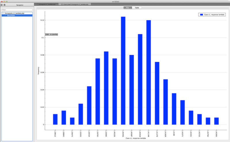
Fig. 6.4.1 Example histogram viewed in Fulcrum.
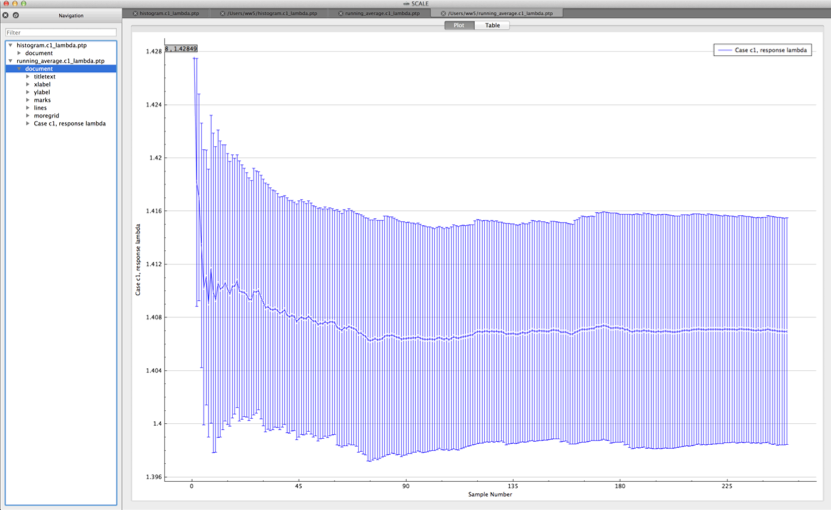
Fig. 6.4.2 Example running average viewed in Fulcrum.
6.4.5.1.4. Response histories
For time-dependent responses, Sampler produces two plots with time-dependent summary data.
standard deviation plot – time-dependent average response with 1-sigma uncertainty bars in directory ${OUTBASENAME}.samplerfiles/histories/history.avg.*
min/max plot – time-dependent average response with min/max error bars in directory ${OUTBASENAME}.samplerfiles/ histories/history.min_max.*
An example of the standard deviation plot is shown Fig. 6.4.3 and the min/max plot in Fig. 6.4.4.
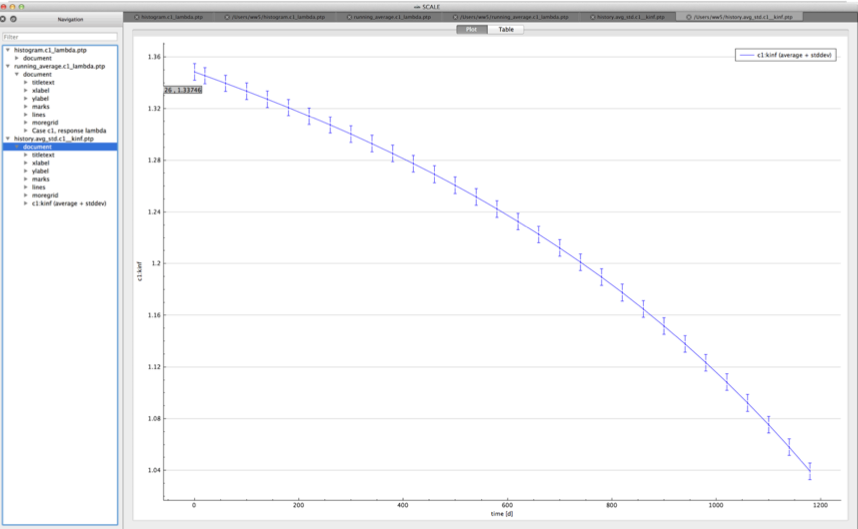
Fig. 6.4.3 Time-dependent average plus standard deviation plot.
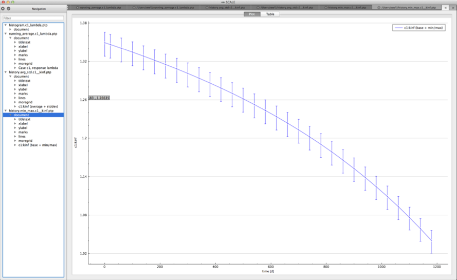
Fig. 6.4.4 Time-dependent average plus min/max plot.
6.4.5.2. Sample problems
The following sample problems demonstrate various computational and output capabilities of Sampler in various situations, for both uncertainty and parametric calculations.
Input files for those sample problems can be found in the samples/input
directory of the SCALE installation. The naming convention for the
inputs is sampler_N.inp, where N is the sample problem number.
The number of samples (n_samples) shown here may vary from the number
included in the sample inputs.
6.4.5.2.1. Sample problem 1
This simple, single-case problem, evaluates uncertainty in eigenvalue for a T-XSDRN calculation of a MOX pincell. Only the cross-sections are perturbed.
=sampler

read parameters
  n_samples=250
  library="xn252"
  perturb_xs = yes
end parameters

read case[c1]
  sequence=t-xsdrn           parm=2region
    pin-cell model with MOX
    xn252
    read comp
      uo2   1 0.95 900 92235 4.5 92238 95.5   end
      zirc2 2 1 600   end
      h2o   3 den=0.75 0.9991 540   end
    end comp
    read cell
      latticecell squarepitch pitch=1.3127 3 fuelr=0.42 1 cladd=0.9500 2 end
    end cell
    read model
    pin-cell model with MOX
    read parm
      sn=16
    end parm
    read materials
      mix=1 com='fuel' end
      mix=2 com='clad' end
      mix=3 com='moderator' end
    end materials
    read geom
      geom=cylinder
      rightBC=white
      zoneIDs 1 2 3 end zoneids
      zoneDimensions 0.42 0.475 0.7406117 end zoneDimensions
      zoneIntervals 3r10 end zoneIntervals
    end geom
    end model
  end sequence
end case

read response[lambda]
  type = grep
  regexp = ":xsdrn.lambda:"
end response

end
The distribution of lambda (k-eff) from sample problem 1 is shown in Fig. 6.4.5.
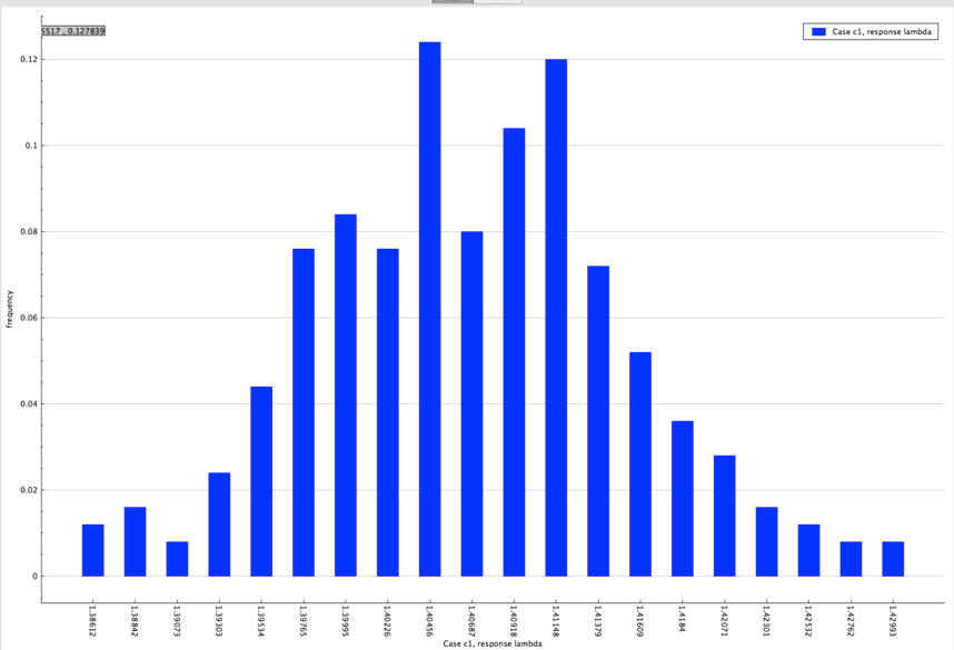
Fig. 6.4.5 Distribution of lambda (k-eff) obtained from sample problem 1.
6.4.5.2.2. Sample problem 2
This problem demonstrates a two-dimensional parametric study (using inline placeholders) for two pincell systems.
=sampler

read parametric
  variables = temp rho end
  n_samples = 3 5 end
end parametric

read case[c1]
  sequence=t-xsdrn           parm=2region
    pin-cell model with MOX
    xn252
    read comp
      uo2   1 0.95 #{temp} 92235 4.5 92238 95.5   end
      zirc2 2 1 600   end
      h2o   3 den=#{rho} 0.9991 540   end
    end comp
    read cell
      latticecell squarepitch pitch=1.8127 3 fuelr=0.45 1 cladd=0.9500 2 end
    end cell
    read model
    pin-cell model with MOX
    read parm
      sn=16
    end parm
    read materials
      mix=1 com='fuel' end
      mix=2 com='clad' end
      mix=3 com='moderator' end
    end materials
    read geom
      geom=cylinder
      rightBC=white
      zoneIDs 1 2 3 end zoneids
      zoneDimensions 0.45 0.475 1.0006117 end zoneDimensions
      zoneIntervals 3r10 end zoneIntervals
    end geom
    end model
  end sequence
end case

read case[c2]
  sequence=t-xsdrn           parm=2region
    pin-cell model with MOX
    xn252
    read comp
      uo2   1 0.95 #{temp} 92235 4.5 92238 95.5   end
      zirc2 2 1 600   end
      h2o   3 den=#{rho} 0.9991 540   end
    end comp
    read cell
      latticecell squarepitch pitch=1.9127 3 fuelr=0.45 1 cladd=0.9500 2 end
    end cell
    read model
    pin-cell model with MOX
    read parm
      sn=16
    end parm
    read materials
      mix=1 com='fuel' end
      mix=2 com='clad' end
      mix=3 com='moderator' end
    end materials
    read geom
      geom=cylinder
      rightBC=white
      zoneIDs 1 2 3 end zoneids
      zoneDimensions 0.45 0.475 1.0406117 end zoneDimensions
      zoneIntervals 3r10 end zoneIntervals
    end geom
    end model
  end sequence
end case

read variable[rho]
  distribution=uniform
  minimum = 0.5
  value = 0.65
  maximum = 0.8
  cases = c1 c2 end
end variable

read variable[temp]
  distribution=uniform
  minimum = 700
  value = 900
  maximum = 1100
  cases = c1 c2 end
end variable

read response[lambda]
  type = grep
  regexp = ":xsdrn.lambda:"
end response

end
The dependency of eigenvalue on coolant density for the two systems is printed to the output file, as shown in Fig. 6.4.6, where the first table shows the temperature and density combinations in the first two columns and the corresponding eigenvalue from case 1 and case 2 in the next two columns. Two summary tables are printed, identifying the conditions of the maximum and minimum for each response, in each case.
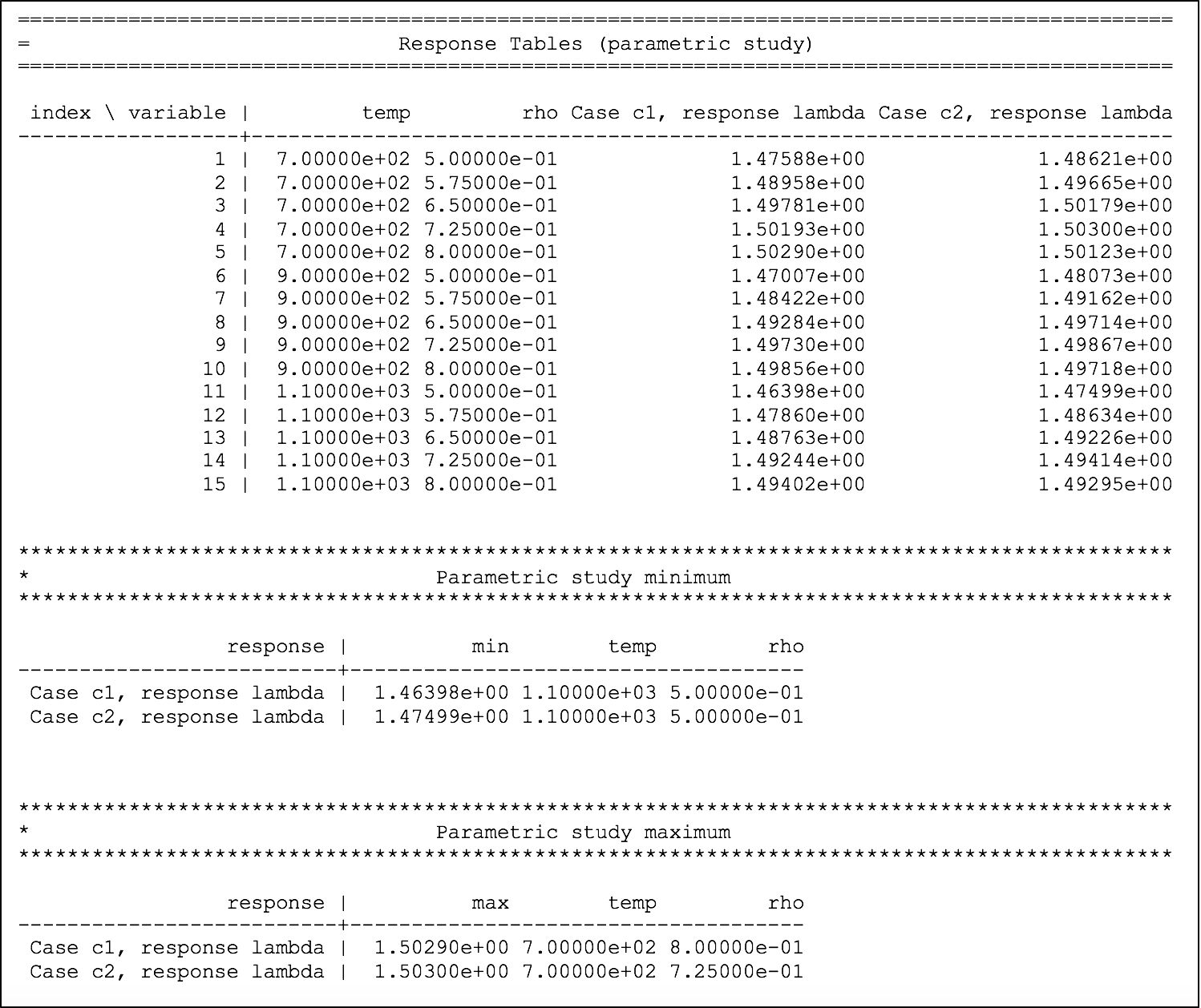
Fig. 6.4.6 Dependency of lambda (k-eff) on coolant density and fuel temperature for sample problem 2.
6.4.5.2.3. Sample problem 3
This sample problem demonstrates enrichment variation using SIREN expressions and dependent variables.
=sampler

read parameters
  n_samples=50
  perturb_geometry=yes
end parameters

read case[sphere]
  sequence=csas5     parm=bonami
  sample problem 14  u metal cylinder in an annulus
  xn252
  read comp
    uranium  1 den=18.69 1 300  92235 94.4 92238 5.6 end
  end comp
  read geom
    global unit 1
      cylinder  1 1 8.89 10.109 0.0 orig 5.0799 0.0
      cylinder  0 1 13.97 10.109 0.0
      cylinder  1 1 19.05 10.109 0.0
  end geom
  end data
  end sequence
  read variable[u235]
    distribution=uniform
    minimum=91.0
    value=94.4
    maximum=95.0
    siren="/csas5/comps/stdcomp/wtpt_pair[id='92235']/wtpt"
  end variable
  read variable[u238]
    distribution=expression
    expression="100.0-u235"
    siren="/csas5/comps/stdcomp/wtpt_pair[id='92238']/wtpt"
  end variable
end case

read response[keff]
  type=grep
  regexp=":kenovi.keff:"
end response
The distribution of the multiplication factor with the specified enrichment distribution is shown in Fig. 6.4.7.
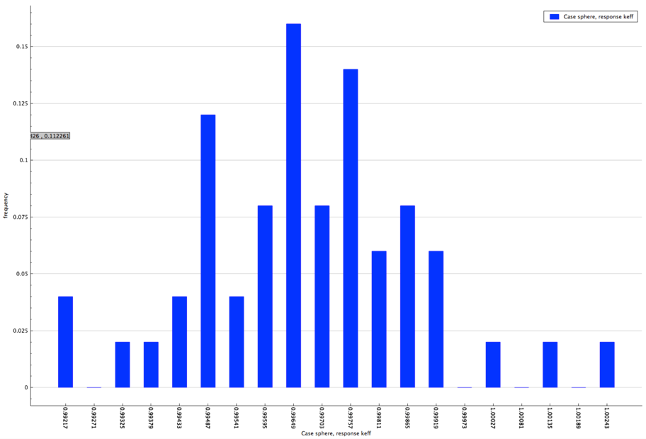
Fig. 6.4.7 Distribution of multiplication factor with sampled enrichment distribution for sample problem 3.
6.4.5.2.3.1. Sample problem 4
Sample problem 4 demonstrates sampling with covariance data for neutron
cross sections and fission product yields. Note that decay sampling does
not work with TRITON at this time due to not using the perturbed ORIGEN
decay libraries directly. Additionally, it demonstrates how to extract
reaction rates from a TRITON case, combining an additional OPUS run with
the opus_plt response.
=sampler

read parameters
  n_samples=100
  library="xn252"
  perturb_xs = yes
  perturb_decay = no
  perturb_yields = yes
end parameters

read case[c1]
  sequence=t-depl  parm=(bonami,addnux=0)
    pincell model
    xn252
    read composition
     uo2         10 0.95 900 92235 3.6 92238 96.4   end
     zirc2       20 1 600   end
     h2o         30 den=0.75 0.9991 540   end
    end composition
    read celldata
      latticecell squarepitch pitch=1.2600 30 fuelr=0.4095 10 cladr=0.4750 20 end
    end celldata
    read depletion
      10
    end depletion
    read burndata
      power=25 burn=1200 nlib=30 end
    end burndata
    read model
    read materials
      mix=10 com="4.5 enriched fuel" end
      mix=20 com="cladding" end
      mix=30 com="water" end
    end materials
    read geom
      global unit 1
        cylinder 10 0.4095
        cylinder 20 0.4750
        cuboid   30 4p0.63
        media 10 1 10
        media 20 1 20 -10
        media 30 1 30 -20
      boundary 30 3 3
    end geom
    read collapse
     150r1 88r2
    end collapse
    read homog
      500 mini 10 20 30 end
    end homog
    read bounds
      all=refl
    end bounds
    end model
  end sequence
  sequence=opus
    typarams=nuclides
    units=fissions
    symnuc=u238 pu239 end
    library="ft33f001.cmbined"
    case = 10
  end sequence
  sequence=opus
    typarams=nuclides
    units=captures
    symnuc=u238 pu239 end
    library="ft33f001.cmbined"
    case = 10
  end sequence
end case

read response[hmgxs]
  type = triton
  data = kinf end
end response

read response[concentrations]
  type=origen_nuclides
  nuclides = u-235 pu-239 pu-240 pu-241 nd-148 sm-149 sm-150 sm-151 cs-133 cs-134 cs-137 end
  mixture = 10
end response

read response[fisrates]
  type = opus_plt
  ndataset = 1
  nuclides = u238 pu239 end
end response

read response[caprates]
  type = opus_plt
  ndataset = 2
  nuclides = u238 pu239 end
end response

end
Plots of various isotopic uncertainties as a function of time are shown in Fig. 6.4.8 for 235U, Fig. 6.4.9 for 239Pu, Fig. 6.4.10 for 240Pu, Fig. 6.4.11 for 241Pu, Fig. 6.4.12 for 148Nd, Fig. 6.4.13 for 150Sm, and Fig. 6.4.14 for 151Sm in terms of the unperturbed with error bars for the minimum and maximum, that is over the 100 samples performed, the minimum value at that time and the maximum value at that time. Note that most isotopes accumulate uncertainty over time, but this is not always the case, e.g. for 151Sm. Two common burnup indicators (measured in spent fuel to infer/confirm burnup) 148Nd and 150Sm show linear increase with time (as expected for a burnup indicator).
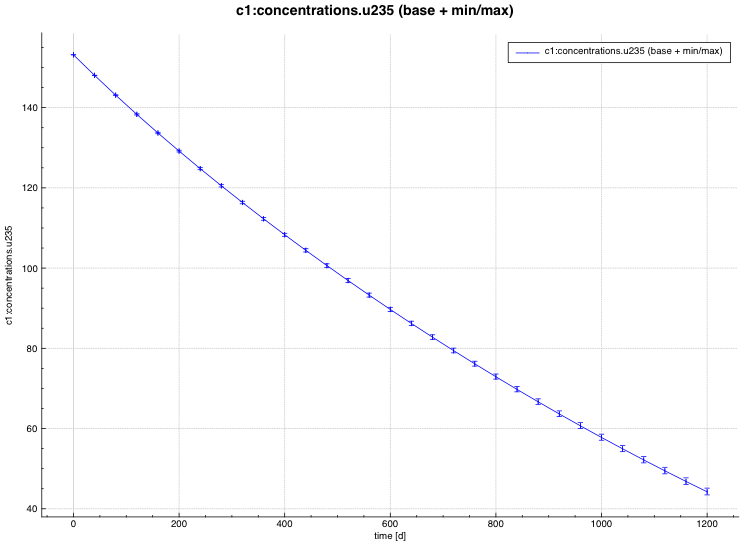
Fig. 6.4.8 Uncertainty in 235U concentration for problem 4.
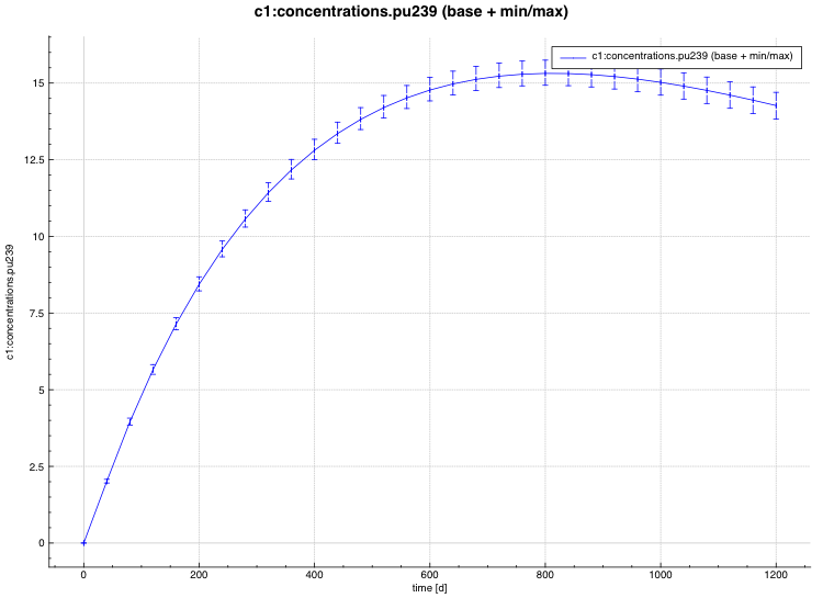
Fig. 6.4.9 Uncertainty in 239Pu concentration for problem 4.
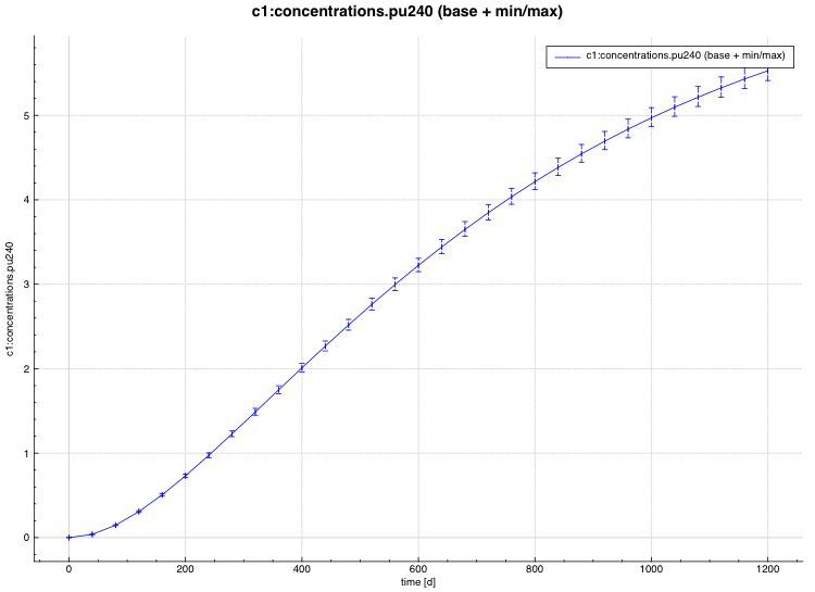
Fig. 6.4.10 Uncertainty in 240Pu concentration for problem 4.
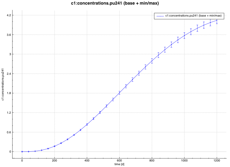
Fig. 6.4.11 Uncertainty in 241Pu concentration for problem 4.
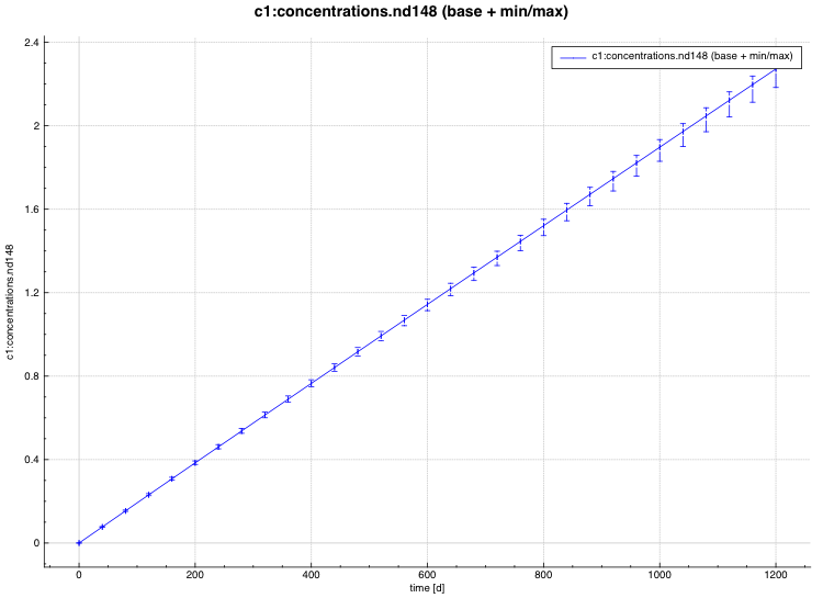
Fig. 6.4.12 Uncertainty in 148Nd concentration for problem 4.
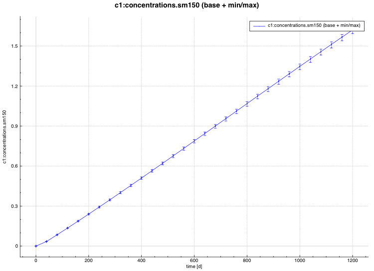
Fig. 6.4.13 Uncertainty in 150Sm concentration for problem 4.
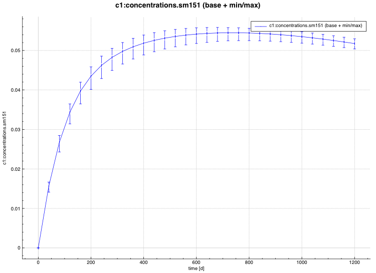
Fig. 6.4.14 Uncertainty in 151Sm concentration for problem 4.
6.4.5.2.4. Sample problem 5
This problem provides an example of two correlated depletion cases. The second “c2” case has a larger pitch and lower enrichment fuel. All data libraries are perturbed.
=sampler

read parameters
  n_samples = 100
  library = "xn252"
  perturb_xs = yes
  perturb_yields = yes
  perturb_decay = yes
end parameters

read case[c1]
  sequence=t-depl  parm=(bonami,addnux=0)
    pincell model
    xn252
    read composition
     uo2         10 0.95 900 92235 3.6 92238 96.4   end
     zirc2       20 1 600   end
     h2o         30 den=0.75 0.9991 540   end
    end composition
    read celldata
      latticecell squarepitch pitch=1.2600 30 fuelr=0.4095 10 cladr=0.4750 20 end
    end celldata
    read depletion
      10
    end depletion
    read burndata
      power=25 burn=1200 nlib=30 end
    end burndata
    read model
    read materials
      mix=10 com="4.5 enriched fuel" end
      mix=20 com="cladding" end
      mix=30 com="water" end
    end materials
    read geom
      global unit 1
        cylinder 10 0.4095
        cylinder 20 0.4750
        cuboid   30 4p0.63
        media 10 1 10
        media 20 1 20 -10
        media 30 1 30 -20
      boundary 30 3 3
    end geom
    read collapse
     150r1 88r2
    end collapse
    read homog
      500 mini 10 20 30 end
    end homog
    read bounds
      all=refl
    end bounds
    end model
  end sequence
end case

read case[c2]
  sequence=t-depl  parm=(bonami,addnux=0)
    pincell model
    xn252
    read composition
     uo2         10 0.95 900 92235 3.6 92238 96.4   end
     zirc2       20 1 600   end
     h2o         30 den=0.75 0.9991 540   end
    end composition
    read celldata
      latticecell squarepitch pitch=1.6600 30 fuelr=0.4095 10 cladr=0.4750 20 end
    end celldata
    read depletion
      10
    end depletion
    read burndata
      power=25 burn=1200 nlib=30 end
    end burndata
    read model
    read materials
      mix=10 com="3.6 enriched fuel" end
      mix=20 com="cladding" end
      mix=30 com="water" end
    end materials
    read geom
      global unit 1
        cylinder 10 0.4095
        cylinder 20 0.4750
        cuboid   30 4p0.83
        media 10 1 10
        media 20 1 20 -10
        media 30 1 30 -20
      boundary 30 3 3
    end geom
    read collapse
     150r1 88r2
    end collapse
    read homog
      500 mini 10 20 30 end
    end homog
    read bounds
      all=refl
    end bounds
    end model
  end sequence
end case

read response[concentrations]
  type=origen_nuclides
  nuclides = u-235 pu-239 pu-240 pu-241 nd-148 sm-149 sm-150 sm-151 cs-133 cs-134 cs-137 end
  mixture = 10
end response

end
The correlation matrix for concentrations at 1200 days of irradiation is shown in Fig. 6.4.15, post-processed with Excel to show high and low correlation coefficients. The bold and underline entries indicate that the each extracted isotope shows a correlation coefficient of 1.0 between the two cases. This means that the two cases are the same in terms of their isotopic response to data perturbations.
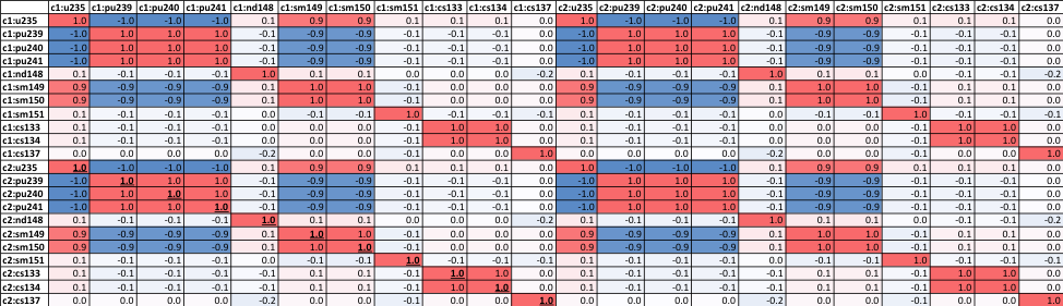
Fig. 6.4.15 Correlation matrix for concentrations in sample problem 5.
6.4.5.2.5. Sample problem 6
Sample problem 6 provides an example of fission yield and decay data sampling. First, COUPLE is run to assemble an ORIGEN library (on file ft33f001) from the perturbed yields and decay data libraries. Burst fission with long decay is then performed by ORIGEN and OPUS is used to extract the fission product decay heat.
=sampler

read parameters
  n_samples = 500
  perturb_yields = yes
  perturb_decay = yes
end parameters

read case[heat]
sequence=couple

0$$ a3 80 21 0 33 e
1$$ a4 1 a18 238 e 1t
9**
 13z 1.25 0.3 223z
2t
done
end sequence
sequence=origens
3$$ 1 1 e t
ft33f001
56$$ 40 1 1 0 -1 a9 0 1 2 1 1 e
t
u235 thermal fission energy release
59**  3.08617e12 f0 e
60** 1e-10 1 1.5 2 4 6 8 10 15 20 40 60 80 100
     150 200 400 600 800 1000 1500 2000 4000 6000 8000 1e4
     1.5e4 2e4 4e4 6e4 8e4 1e5
     1e6 1e7 1e8 1e9 1e10 1e11 1e12 1e13
61** f1e-14
67$$ a47 1 0 1 e
68$$ a2 1 e
73$$ 922350
74** 1
75$$ 2
80$$ 0 f1
t
ft71f001
end sequence
sequence=opus
  library="ft33f001"
  units=watts
  libtype=fiss
  minposition=2
end sequence
end case

read response[heat]
  type=opus_plt
  ndataset=0
  nuclides=total end
end response

end
The total decay heat with the uncertainty is shown in Table 6.4.7 and Fig. 6.4.16.

|
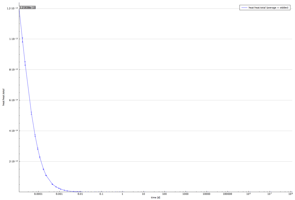
Fig. 6.4.16 Decay heat and uncertainties from sample problem 6.
6.4.5.2.6. Sample problem 7
Sample problem 7 illustrates an example of a shielding parametric study with MAVRIC. It also demonstrates usage of the grep response for both response value and uncertainty.
=sampler

read parameters
  n_samples = 50
end parameters

read parametric
  variables = thick end
end parametric

read case[graphite]
sequence=mavric
Monaco/MAVRIC Training - Exercise 3. Graphite Shielding Measurements Revisited
v7-27n19g

'-------------------------------------------------------------------------------
' Composition Block - standard SCALE input
'-------------------------------------------------------------------------------
read composition
    para(h2o)    3         1.0 293.0 end
    carbon       4 den=1.7  1.0 300.0 end
end composition

'-------------------------------------------------------------------------------
' Geometry Block - SCALE standard geometry package (SGGP)
'-------------------------------------------------------------------------------
read geometry
    global unit 1
        cuboid  1   25.0 -25.0  25.0 -25.0   25.0 -25.0
        cone    2  10.35948  25.01   0.0 0.0   rotate  a1=-90 a2=-90 a3=0
        cuboid  3   #{x90}  70.0  40.0 -40.0   40.0 -40.0
        cuboid 99  120.0 -30.0  50.0 -50.0   50.0 -50.0
        media 3 1  1 -2
        media 0 1  2
        media 4 1  3
        media 0 1  99 -1  -2 -3
    boundary 99
end geometry

'-------------------------------------------------------------------------------
' Definitions Block
'-------------------------------------------------------------------------------
read definitions
    location 1
        position 110 0 0
    end location
    response 5
        title="ANSI standard (1977) neutron flux-to-dose-rate factors"
        specialDose=9029
    end response
    distribution 1
        title="Cf-252 neutrons, Watt spectrum a=1.025 MeV and b=2.926/MeV"
        special="wattSpectrum"
        parameters 1.025 2.926 end
    end distribution
    gridGeometry 7
        title="large meshes in paraffin, 5 cm mesh for shield thicknesses"
        xLinear 5 -25 25
        xLinear 12 30 #{x90}
        xplanes 100 110 120 -30 end
        yplanes -50 -40 40 50 end
        yLinear 7 -35 35
        zplanes -50 -40 40 50 end
        zLinear 7 -35 35
    end gridGeometry
end definitions

'-------------------------------------------------------------------------------
' Sources Block
'   Cf-252 neutrons, Watt fission spectrum model
'   with a=1.025 MeV and  b=2.926/MeV
'-------------------------------------------------------------------------------
read sources
    src 1
        title="Cf-252 neutrons, Watt fission spectrum model"
        strength=4.05E+07
        cuboid  0.01 0.01  0 0  0 0
        neutrons
        eDistributionID=1
    end src
end sources

'-------------------------------------------------------------------------------
' Tallies Block
'-------------------------------------------------------------------------------
read tallies
    pointDetector 1
        title="center of detector"
        neutron
        locationID=1
        responseID=5
    end pointDetector
    meshTally 1
        title="example mesh tally"
        neutron
        gridGeometryID=7
        responseID=5
        noGroupFluxes
    end meshTally
end tallies

'-------------------------------------------------------------------------------
' Parameters Block
'-------------------------------------------------------------------------------
read parameters
    randomSeed=00003ecd7b4e3e8b
    library="v7-200n47g"
    perBatch=10000 batches=10
    fissionMult=0   noPhotons
end parameters

'-------------------------------------------------------------------------------
' Importance Map Block
'-------------------------------------------------------------------------------
read importanceMap
    adjointSource 1
        locationID=1
        responseID=5
    end adjointSource
    gridGeometryID=7
    macromaterial
      mmTolerance=0.01
    end macromaterial
end importanceMap

end data
end sequence

read variable[thick]
  value = 20
  minimum = 10
  maximum = 30
  distribution = uniform
end variable

read variable[x90]
  distribution = expression
  expression = "thick+70"
end variable

end case

read response[flux]
  type = grep
  regexp = "total flux[[:space:]]+:scale.number:"
  regexp = ":scale.number:"
end response

end
Flux dependence on the shielding thickness is shown in Fig. 6.4.17.
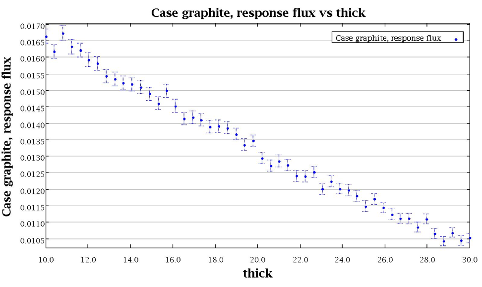
Fig. 6.4.17 Flux as a function of shielding thickness for sample problem 7.
6.4.6. SCALE Input Retrieval ENgine (SIREN)
SIREN (SCALE Input Retrieval ENgine) provides a hierarchical representation of SCALE input and enables access to individual input components or sets of related input parameters. SIREN sorts the contents of supported SCALE input sequences into a tree structure so that every component in a SCALE input can be accessed using an XPath designation. The SIREN package is used by the SCALE super-sequence Sampler to select individual components within an input file, perturb the parameter in memory, and write the perturbed input to a new file. In this way, components within an input file can be perturbed without modification to the original input file, which can be maintained as a read-only file under configuration control for quality assurance purposes.
To explore the use of SIREN expressions, two utilities are available in the SCALE bin directory. The utilities are the executables “InputViewer” and “InputSelector.” The InputViewer utility accepts a SCALE input file and outputs the XPath designation for each component of that input file. The InputSelector utility accepts a SCALE input file and a SIREN select statement and then outputs the part of the input file specified by the SIREN select statement. The remainder of this section provides practical examples in the use of SIREN select statements to designate specific components of a SCALE input.
A simple CSAS6 input file, which models a sphere of HEU, is used to show how to use SIREN select statements to access specific portions of a SCALE input. The contents of the example CSAS6 input file are shown below.
=csas6
sample problem 6  bare 93.2% U sphere, eighth sphere w/ mirror albedo
v7-238
read comp
  uranium  1 den=18.76 1 293 92235 93.2 92238 5.6 92234 1.0 92236 0.2 end
end comp
read geometry
  global unit 1
    sphere 10  8.741  chord +x=0.0  chord  +y=0.0  chord +z=0.0
    cuboid   20  8.741 0.0 8.741 0.0 8.741 0.0
    media  1 1 10      vol=2797.5121
    media  0 1 20 -10  vol=2545.3424
    boundary 20
end geometry
read bounds
  -fc=mirror
end bounds
end data
end
The InputViewer utility is used to view the contents of the example input file with their respective XPath designations. The utility accepts the path to the input file as an argument so that the usage is:
$ InputViewer inputfile
A portion of the output from InputViewer is shown below; this portion corresponds to the material definition in the example input file. Notice that each component of the composition has a specific XPath designation. For instance, the “wtptPair” has several pieces of information (ids for each component and the weight percent for that component). To gain access to a specific component, the InputSelector utility is introduced below.
/csas6/comps
/csas6/comps/decl(read comp)
/csas6/comps/stdcomp
/csas6/comps/stdcomp/name(uranium)
/csas6/comps/stdcomp/mixture(1)
/csas6/comps/stdcomp/roth
/csas6/comps/stdcomp/roth/decl(den)
/csas6/comps/stdcomp/roth/assign(=)
/csas6/comps/stdcomp/roth/value(18.76)
/csas6/comps/stdcomp/vf(1)
/csas6/comps/stdcomp/temp(293)
/csas6/comps/stdcomp/wtpt_pair
/csas6/comps/stdcomp/wtpt_pair/id(92235)
/csas6/comps/stdcomp/wtpt_pair/wtpt(93.2)
/csas6/comps/stdcomp/wtpt_pair
/csas6/comps/stdcomp/wtpt_pair/id(92238)
/csas6/comps/stdcomp/wtpt_pair/wtpt(5.6)
/csas6/comps/stdcomp/wtpt_pair
/csas6/comps/stdcomp/wtpt_pair/id(92234)
/csas6/comps/stdcomp/wtpt_pair/wtpt(1.0)
/csas6/comps/stdcomp/wtpt_pair
/csas6/comps/stdcomp/wtpt_pair/id(92236)
/csas6/comps/stdcomp/wtpt_pair/wtpt(0.2)
/csas6/comps/stdcomp/term(end)
/csas6/comps/term(end comp)
To explore how SIREN select statements are used, the InputSelector utility is used for a few cases with the example CSAS6 input file. Suppose the 235U weight percent needed to be accessed for perturbation; the SIREN expression to access the 235U weight percent is as follows:
Long form:
'/csas6/comps/stdcomp/wtpt_pair[id="92235"]/wtpt'
Short form:
'///wtpt_pair[id="92235"]/wtpt'
This statement tells SIREN to look for the weight percent with an ID of 92235 in the weight percent pair. A short form of the select statement (designated by the triple slash) can be used when there are unique qualities about a component; for instance, there is only a single material with an ID of 92235, so the weight percent pair must belong to that material. There are many combinations of select statements that can point to a specific input component, and the developers suggest using the InputSelector utility to familiarize oneself with this capability. The usage of InputSelector is:
$ InputSelector inputfile quoted_Select_Statement
Below is the screen output from the InputSelector with the example CSAS6 input file and the select statement for the 235U weight percent.
---- 1 nodes selected with statement '///wtpt_pair[id='92235']/wtpt' ----
1) /csas6/comps/stdcomp/wtpt_pair/wtpt
93.2
The output from InputSelector shows that the select statement points to a single component in the SCALE input, which is indeed the value for the 235U weight percent. There are cases where a select statement points to a portion of the input that has multiple components and the select statement may need to be refined to point to a specific component. For instance, the cuboid defined in the geometry section of the input has multiple dimensions (+x, -x, +y, -y, etc.). By using the select statement below, the dimensions of the cuboid are shown
'//cuboid/[id="20"]/dimensions'
The output from using InputSelector with this select statement is shown below.
---- 1 nodes selected with statement '//cuboid/[id="20"]/dimensions' ----
1) /csas6/geometry/global_unit/cuboid/dimensions

8.741 0.0 8.741 0.0 8.741 0.0
The output from InputSelector shows six values, which correspond to the dimensions of the cuboid (+x, x, +y, -y, +z, -z faces). To select a single dimension, the select statement should include which component is desired. For instance, to select the height of the cuboid the select statement becomes:
'//cuboid/[id="20"]/dimensions/plus_z'
In the same way, the radius of the sphere can be selected using the SIREN expression that identifies the radius of a sphere with an ID of 10:
'//sphere/[id="10"]/dimensions/r'
The output from InputSelector is shown below.
---- 1 nodes selected with statement '//sphere/[id="10"]/dimensions/r' ----
1) /csas6/geometry/global_unit/sphere/dimensions/r

8.741
There are scenarios where there is no unique or obvious identifier for a component. As an example, the media volume can utilize an array index to retrieve the volume value.
'//media/volume/value'
The output from InputSelector illustrates both media’s volume value are selected below.
---- 2 nodes selected with statement '//media/volume/value' ----
1) /csas6/geometry/global_unit/media/volume/value
2797.5121
2) /csas6/geometry/global_unit/media/volume/value
2545.3424
The printed index (1) can be utilized to narrow the selection.
‘//media[1]/volume/value’
Here the first media is selected and subsequently, the media’s volume value, removing the selection of the second media entirely. The output from InputSelector is shown below.
---- 1 nodes selected with statement '//media[1]/volume/value' ----
1) /csas6/geometry/global_unit/media/volume/value
2797.5121
For the sake of completeness, the following example illustrates selection of the media’s volume value via the mixture’s value comparator.
'//media[mixture="1"]/volume/value'
This illustrates the first media’s unique mixture component can be used to select the volume for the first media. The output from InputSelector is shown below.
---- 1 nodes selected with statement '//media[mixture="1"]/volume/value' ----
1) /csas6/geometry/global_unit/media/volume/value

2797.5121
The above examples were intended to provide users with an idea of how to use SIREN select statements to access specific components within a SCALE input. The select statements are primarily used in cases where the input is to be perturbed by the Sampler super-sequence, but modification to the original input is not desirable. The recommended way to ensure that the select statements are correct is to use the InputSelector utility to check that a select statement points to the correct input component.
For viewing the input paths, an alternative to the InputViewer command line utility is available within the Fulcrum graphical user interface (GUI). By clicking on the Run Button drop-down and selecting “Input Listing” as shown in Fig. 6.4.18, the full listing of the current input file is displayed in the “Messages” box. Also, notice the path is displayed in the bottom left corner for the input component located at the cursor.
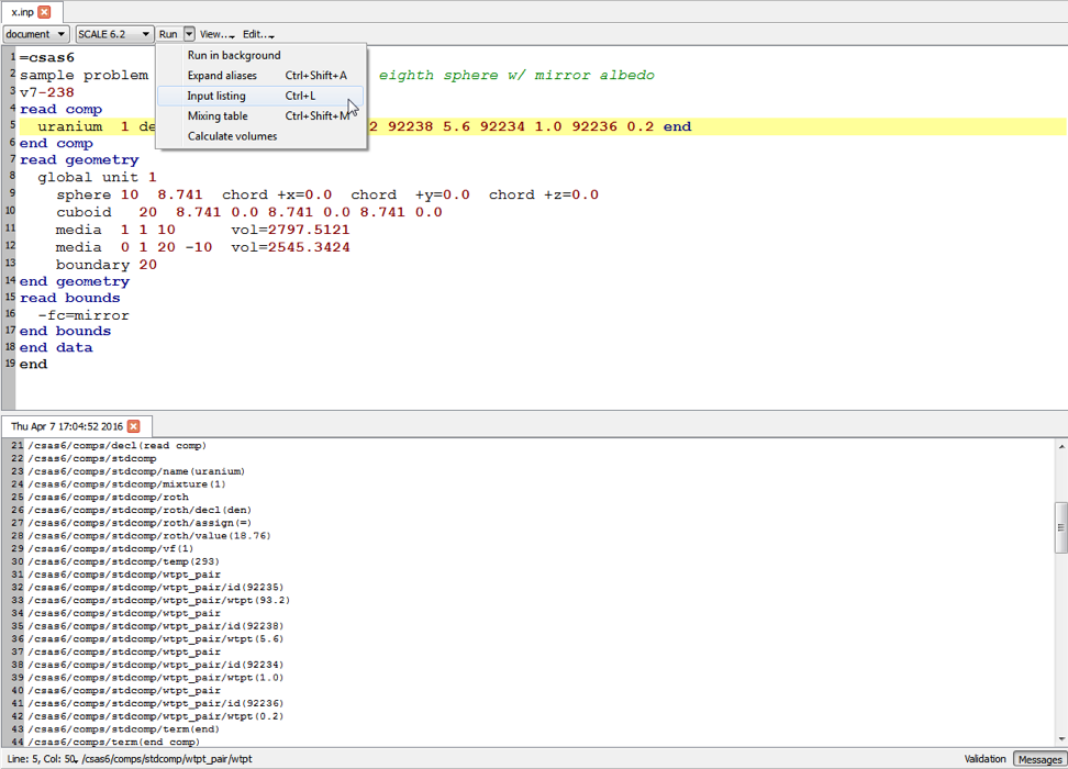
Fig. 6.4.18 Input Listing in Fulcrum.
A table of SIREN expressions is as follows.
Expressions |
Description |
Examples |
|---|---|---|
component |
Component match. |
csas6 |
/ |
Component separator. When the expression begins with this, it selects the root of the document. |
csas6/xslib / |
// |
This expression is the ‘Any Child’ select. |
csas6//uranium // |
[index] |
Array index selector. When an array of objects has been selected, this expression selects the object at the given index. |
csas6/ geometry/global_unit/media**[1]** |
[sindex:eindex] |
Subarray index selector. When an array of objects has been selected, this expression selects a subarray. |
csas6/ comps/stdcomp/uranium/wtpt_pair**[2:3]** |
[sindex:eindex:stride] |
Subarray index selector. When an array of objects has been selected, this expression selects a subarray and subsequently components stride apart. |
csas6/comps/stdcomp/uranium/wtptPair**[1:4:2]** |
* |
Component wild card. This can only be used in place of a component or to wild card the remainder of a component. |
csas6/read comp/* csas6/read comp/ur* |
6.4.7. Expression Operators and Functions for Sampler
The expression engine utilized by Sampler supports all basic mathematical and logical operators, as well as a number of functions. Logical expressions and functions evaluate to the number 1 for true, and the number 0 for false.
Operator |
Description |
Example |
|---|---|---|
+ |
Addition |
3+3, x+y |
+ |
Unary Plus |
+3, +(-3), +x |
- |
Subtraction |
3-3, x-y |
- |
Unary Minus |
-3, -(3+3), -x |
* |
Multiplication |
3*3, x*y |
/ |
Division |
3/3, x/y |
% |
Modulo |
3%3, x%y |
^ |
Power |
3^3, x^y |
== |
Equal to |
3==3, x==y |
!= |
Not equal to |
3!=3, x!=y |
< |
Less than |
3<3, x<y |
> |
Greater than |
3>3, x>y |
<= |
Less than or equal to |
3<=3, x<=y |
>= |
Greater than or equal to |
3>=3, x>=y |
and |
Left is true and right is true |
1 and 1 , x==y and y==z |
or |
Left is true or right is true |
1 or 1, x==y or y==z |
nand |
Not and |
1 nand 1, 1 nand 0, x nand y |
xor |
Exclusive or |
1 xor 1, 1 xor 0, x xor y |
nor |
Not or |
1 nor 1, 1 nor 0, x nor y |
abs(x) |
Absolute value |
abs(1),abs(-1),abs(x) ,abs(y) |
min(x,…n) |
Minimum of values |
min(1),min(1,2,3,4,5, x,y),etc |
max(x,…n) |
Maximum of values |
max(1),max(1,2,3,4,5, x,y),etc |
avg(x,…n) |
Average of values |
avg(1),avg(1,2,3,4,5, x,y),etc |
Sum(x,…n) |
Summation of values |
sum(1),sum(1,2,3,4,5, x,y),etc |
mul(x,…n) |
Multiply values |
mul(1),mul(1,2,3,4,5, x,y),etc |
floor(x) |
Floor of the value |
floor(1)=1, floor(-1.0)=-1.0, floor(-1.1)=-2.0 |
ceil(x) |
Ceiling of the value |
ceil(1)=1,ceil(-1.1)= -1 |
round(x) |
Round the value to nearest integer |
round(1.1)=1,round(1.5)=2,round(1.9)=2 |
roundn(x,n) |
Round the value to the nth decimal position |
roundn(1.15,1)= 1.2, roundn(1.519,2)= 1.52 |
cos(x) |
Cosine of the value |
cos(0.0)=1 |
sin(x) |
Sine of the value |
sin(0.0)=0 |
tan(x) |
Tangent of the value |
tan(0.0)=0 |
sec(x) |
Secant of the value |
sec(0.0)=1 |
csc(x) |
Cosecant of the value |
csc(1.0)= 1.1884 |
cot(x) |
Cotangent of the value |
cot(1.0)= 0.642093 |
sinh(x) |
Hyperbolic sine of the value |
sinh(1.0)= 1.1752 |
cosh(x) |
Hyperbolic cosine of the value |
cosh(1.0)= 1.54308 |
tanh(x) |
Hyperbolic tangent of the value |
tanh(1.0)= 0.761594 |
log(x) |
Natural log of the value |
log(2.7182818)=1 |
log10(x) |
Common log of the value |
log10(10.0)=1 |
exp(x) |
Exponential of the value |
exp(1)=2.7182818 |
clamp(l,x,u) |
Clamp the value x between lowerbound l and upperbound u |
clamp(-1,1,+1)=1,clamp(-1,-5,+1)=-1 |
inrange(l,x,u) |
Determine if value x is greater than or equal to lowerbound l, and less than or equal to upperbound u |
inrange(-1,1,+1)=1,inrange(-1,-5,+1)=0 |
sgn(x) |
Determine the sign of x. |
sgn(+1)=1,sgn(-1)=-1, sgn(0)=0,sgn(5)=1 |
sqrt(x) |
Square Root of the value |
sqrt(1)=1,sqrt(4)=2 |
root(x,y) |
Root of x given y |
root(4,2)=2,root(8,3)=2 |
true |
Constant true value |
true |
false |
Constant false value |
False |
if(condition,true,false) |
If function that evaluates the condition. If true, the true value is substituted, else the false value is substituted |
if( x > y, x, y) = x |
6.4.8. Guidelines for Running Sampler in Parallel
Sampler calculations consist of three basic steps:
generate N perturbed input files and libraries,
run N independent SCALE jobs, and
analyze N results sets.
At this time, the preferred way of performing Sampler calculations is to use run_cases=no (in the parameters block) and perform step 2 above outside of Sampler, i.e. using scripting or your system’s queuing system to launch the N SCALE jobs. The “${OUTBASENAME}.samplerfiles” directory that Sampler creates in step 1 will contain all the perturbed input files. Each of these input files should be run as a separate SCALE job. When all jobs are complete, Sampler should be run again (still with run_cases=no). Sampler will see that all jobs have completed, and perform the analysis in step 3. The Sampler sample problem 8 is a quick-running calculation that can be used to test and, if necessary adjust, the manual 3-step scheme described above on your system.
However, for small jobs that fit on a single node, threading can be used. To launch a Sampler calculation with 5 parallel threads, one would issue the following from the command line:
scalerte –r –I 5 –m sample_8.inp
This will perform all 3 steps of the Sampler process.
- 1
ÚJV Řež, a. s., Czech Republic
- 2
Gesellschaft fur Anlagen- und Reaktorsicherheit (GRS)
- 3
Texas A&M University
References
- SAMPLER-BWAW22
Friederike Bostelmann, Dorothea Wiarda, Goran Arbanas, and William A. Wieselquist. Extension of SCALE/Sampler's sensitivity analysis. Annals of Nuclear Energy, 165:108641, 2022. doi:10.1016/j.anucene.2021.108641.
- SAMPLER-BHNS10
O. Buss, A. Hoefer, J. C. Neuber, and M. Schmid. Hierarchical Monte-Carlo Approach to Bias Estimation for Criticality Safety Calculations . In Proceedings of PHYSOR 2010, Advances in Reactor Physics to Power the Nuclear Renaissance. Pittsburgh, PA (USA), 5 2010.
- SAMPLER-HMAK20
Dongli Huang, Ugur Mertyurek, and Hany Abdel-Khalik. Verification of the sensitivity and uncertainty-based criticality safety validation techniques: ornl’s scale case study. Nuclear Engineering and Design, 361:110571, 2020. doi:https://doi.org/10.1016/j.nucengdes.2020.110571.
- SAMPLER-KHK94
B. Krzykacz, E. Hofer, and M. Kloos. A Software System for Probabilistic Uncertainty and Sensitivity Analysis of Results from Computer Models. In Proc. International Conference on Probabilistic Safety Assessment and Management (PSAM-II). San Diego, CA (USA), 1994.
- SAMPLER-PFG15
M. T. Pigni, M. W. Francis, and I. C. Gauld. Investigation of Inconsistent ENDF/B-VII.1 Independent and Cumulative Fission Product Yields with Proposed Revisions. Nuclear Data Sheets, 123:231–236, 2015. doi:https://doi.org/10.1016/j.nds.2014.12.040.
- SAMPLER-RWJ+11(1,2)
B. T. Rearden, M. L. Williams, M. A. Jessee, D. E. Mueller, and D. A. Wiarda. Sensitivity and Uncertainty Analysis Capabilities and Data in SCALE. Nuclear Technology, 2(174):236–288, 2011.
- SAMPLER-WIJ+13
M. L. Williams, G. Ilas, M. A. Jessee, B. T. Rearden, D. Wiarda, W. Zwermann, L. Gallner, M. Klein, B. Krzykacz-Hausmann, and A. Pautz. A Statistical Sampling Method for Uncertainty Analysis with SCALE and XSUSA. Nuclear Technology, pages 515–526, 2013.