4.4. MAVRIC Advanced Features
This appendix contains information on several advanced features that are still under development or are non-standard use of the MAVRIC sequence.
4.4.1. Alternate normalization of the importance map and biased source
The importance map and biased source implemented in MAVRIC are only functions of space and energy. The importance for a specific location and energy represents the average over all directions. For applications involving a collimated beam source, a space/energy importance map may not be representative of the true importance of the particles as they stream away from the source.
As an example, consider a 14.1 MeV active interrogation beam source 1 meter from a small spherical boat containing illicit nuclear material. The objective is to compute the fission rate in the nuclear material. To create the biasing parameters, an adjoint source is located within the nuclear material and the resulting importance map is shown in Fig. 4.4.1. Note that in both the air and water, the importances change with distance from the ship, but for the beam source, the importance (to causing a fission in the nuclear material) anywhere along the beam should be the same, since there is little chance a 14.1 MeV neutron will interact with the air before striking the ship.
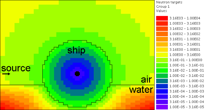
Fig. 4.4.1 Importance map computed using standard CADIS.
The CADIS algorithm has done exactly what it was supposed to: it made a space/energy importance map and normalized it such that the target weight where the 14.1 MeV source particles are born is 1. The problem with this is that the source particles will stream towards the ship and strike the hull where the target weight is 0.092. Since source particles have little chance of interacting in the air, the weight windows are not used to split the particle as they travel towards the ship. When source particles cross into the ship, they are split by a factor of 11 to match the target weight. For this example, splitting each particle by a factor of 11 once they strike the ship is not so bad, but for longer distances, this will result in much larger splits. For a polyenergetic source, this could lead to undersampling of the source and could result in higher variances.
To remedy this problem when using beam sources, the normalization of the importance map and biased source should not be done at the source location but instead at the point where the source particles first interact with the ship. The keyword “shiftNormPos \(\Delta\)Delta`y \(\Delta\)Delta`x, \(\Delta\)Delta`z when the biased source and importance map are developed. For the Monaco Monte Carlo calculation, the source is returned to its normal position. The source input for the above problem would then be
read sources
    src 1
        title="14.1 DT neutrons - collimated"
        strength=1e30
'       (true source position)
        sphere 0 origin x=-195 y=0 z=0
'       (a mono-energetic 14.1 MeV distribution)
        eDistributionID=1
        direction 1.0 0.0 0.0
'       (a 2° beam )
        dDistributionID=2
'       (just inside the hull)
        shiftNormPos 107.7 0.0 0.0
    end src
end sources
where the shift moves the source position from x = -195 to x = -87.3, just inside the hull. The resulting target weights are shown in Fig. 4.4.2 The source particles are born with weight 1 in a location with a target weight 10.9. The particle weight is not checked until the particle crosses into the hull, where the target weight is 1.0.
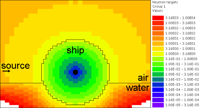
Fig. 4.4.2 Targets weights using the “shiftNormPos” keyword.
Other options to manipulate the importance map for special situations include the “mapMultiplier=f” keyword (in the importanceMap block or the biasing block), which will multiply every target weight by the factor f, and the keyword “noCheckAtBirth” in the parameters block will prevent the weight windows from being applied to source particles when they are started. When used in the MAVRIC sequence, the “shiftNormPos” capability automatically adds “noCheckAtBirth” to the Monaco input that is created.
4.4.2. Importance maps with directional information
In MAVRIC, the CADIS method is implemented in space and energy, but in general, it could also include particle direction as well. This formulation would be the following:
- True source:
- Desired response:
- Adjoint flux using \(q^{+}\left( \overrightarrow{r},E,\widehat{\Omega} \right) = \ \sigma \left( \overrightarrow{r},E,\widehat{\Omega} \right)\):
- Estimate of detector response
- Biased source:
- Target weight windows:
For a system using a deterministic method to compute the adjoint fluxes, this completely general, space/energy/angle, approach presents many difficulties in implementation, namely,
dealing with the amount of memory required for a \(\left( \overrightarrow{r},E,\widehat{\Omega} \right)\) importance map in memory,
interpolating the importance for particle directions in between quadrature angles, and
expressing the biased source in a form suitable for a general MC code since the above biased source is, in general, not separable.
4.4.2.1. Approaches incorporating directional information
Completely general space/energy/angle CADIS is most likely too difficult to implement and may not be necessary for most applications. In most real problems that involve directionally dependent source distributions, the directional dependence is azimuthally symmetric about some reference direction, \(\widehat{d}\). The angular distribution, \(q_{i}\left( \widehat{\Omega} \right)\), can be expressed as the product of the uniform azimuthal distribution and a polar distribution about reference direction \({\widehat{d}}_{i}\) giving \(\frac{1}{2\pi}q_{i}\left( \widehat{\Omega} \bullet {\widehat{d}}_{i} \right)\). The geometric size of these sources tends to be small, allowing each source distribution to be expressed as the product of two separable distributions: \(q_{i}\left( \overrightarrow{r},E,\widehat{\Omega} \right) \cong q_{i}\left( \overrightarrow{r},E \right)\ q_{i}\left( \widehat{\Omega} \right)\).
What is needed is a CADIS method that (1) can account for the importance of a particle traveling in a certain direction; (2) can be cast as a simple modification of the space/energy CADIS method using \(\overline{w}\left( \overrightarrow{r},E \right)\) and \(\widehat{q}\left( \overrightarrow{r},E \right)\); and (3) is simpler than the full space/angle/energy approach. This can be done starting with the approximation that the angular component of the adjoint flux \(\psi^{+}\left( \overrightarrow{r},E,\widehat{\Omega} \right)\) is separable and symmetric about the average adjoint current direction \(\widehat{n}\left( \overrightarrow{r},E \right)\), such that
This is similar to the AVATAR approach [MAV-AppC-VRUS97] but with explicitly including the azimuthal distribution so that the standard definition \(\int_{}^{}{\phi^{+}\left( \overrightarrow{r},E \right)\ \frac{1}{2\pi}f\left( \widehat{\Omega} \bullet \widehat{n} \right)\ d\widehat{\Omega}} = \phi^{+}\left( \overrightarrow{r},E \right)\) applies. The probability distribution function \(f\left( \mu \right)\) describing the shape of the azimuthally symmetric current at \(\left( \overrightarrow{r},E \right)\) has the form of
with the single parameter \(\lambda\left( \overrightarrow{r},E \right)\) determined from \(\overline{\mu}\left( \overrightarrow{r},E \right)\), the average cosine of scatter.
From this, we can propose that weight window targets be developed that are inversely proportional to the approximation of the adjoint angular flux:
where \(k\) is the constant of proportionality that will be adjusted to make the importance map consistent with the biased source(s). Two methods will be examined here, one without and one with biasing of the source directional dependence.
For both of the methods, the SN code Denovo was modified to report not only the adjoint scalar fluxes, \(\phi^{+}\left( \overrightarrow{r},E \right)\), but also the adjoint net currents in \(x\), \(y\), and \(z\) directions: \(J_{x}\left( \overrightarrow{r},E \right)\), \(\ J_{y}\left( \overrightarrow{r},E \right)\), and \(J_{z}\left( \overrightarrow{r},E \right)\). These currents are used to find \(\widehat{n}\left( \overrightarrow{r},E \right)\) and \(\lambda\left( \overrightarrow{r},E \right)\). The following methods have been developed so that the standard CADIS routines can be used to compute space/energy quantities of the response per unit source \(R\), the weight window target values \(\overline{w}\left( \overrightarrow{r},E \right)\), and biased source \(\widehat{q}\left( \overrightarrow{r},E \right)\) with just the adjoint scalar fluxes. These quantities are then modified by the directional information.
4.4.2.2. Directionally dependent weight windows without directional source biasing
It is proposed that the biased source \(\widehat{q}\left( \overrightarrow{r},E,\widehat{\Omega} \right)\) should be proportional to both the true source distribution and the space/energy component of the adjoint flux:
where the constant of proportionality, \(R\), is determined by forcing \(\widehat{q}\left( \overrightarrow{r},E,\widehat{\Omega} \right)\) to be a pdf. Since the angular component of the adjoint flux is not included, the directional distribution of the biased source will be exactly the same as the true source. Note that this approach would be exact for cases where no directional biasing could be applied — beam sources.
For multiple sources (each with a probability distribution function \(q_{i}\left( \overrightarrow{r},E \right)\) and a strength \(S_{i}\), giving a total source strength of \(S = \sum_{}^{}S_{i}\)), the user is required to provide one point in phase space \(\left( {\overrightarrow{r}}_{i},E_{i},{\widehat{\Omega}}_{i} \right)\) for each source \(i\) that is representative of that entire source where the biased source will match the target weight windows. For each source, a vector \({\widehat{n}}_{i} = \widehat{n}\left( {\overrightarrow{r}}_{i},E_{i} \right)\) is computed using that point. For the general case of multiple sources, the biased source sampling distribution, the biased source distributions, and the weight windows are computed using
\(R_{i} = \iint_{}^{}{q_{i}\left( \overrightarrow{r},E\right)\ \phi^{+}\left( \overrightarrow{r},E \right)} dE \ dr \ \ \ \ \ \ \ \ \ \text{(estimated response from source} \ i)\)
\(\widehat{p}\left( i \right) = \frac{{S_{i}R}_{i}\ f\left( {\widehat{\Omega}}_{i} \bullet {\widehat{n}}_{i} \right)}{\sum_{}^{}{{S_{i}R}_{i}\ f\left( {\widehat{\Omega}}_{i} \bullet {\widehat{n}}_{i} \right)}} \ \ \ \ \ \ \ \text{(biased sampling of source} \ i)\)
\({\widehat{q}}_{i}\left(\overrightarrow{r},E,\widehat{\Omega} \right) \ = \ \frac{1}{R_{i}}q_{i}\left( \overrightarrow{r},E \right)\ \phi^{+}\left( \overrightarrow{r},E \right)\ \frac{1}{2\pi}q_{i}\left( \widehat{\Omega} \bullet {\widehat{d}}_{i} \right) \ = \ {\widehat{q}}_{i}\left( \overrightarrow{r},E\right)\ \frac{1}{2\pi}q_{i}\left( \widehat{\Omega} \bullet {\widehat{d}}_{i} \right)\)
\(\overline{w}\left( \overrightarrow{r},E,\widehat{\Omega} \right) \ \ \ = \ \ \ \frac{\sum_{}^{}{{S_{i}R}_{i}\ f\left( {\widehat{\Omega}}_{i} \bullet {\widehat{n}}_{i} \right)}}{S\phi^{+}\left( \overrightarrow{r},E \right)}\frac{1}{\ f\left( \widehat{\Omega} \bullet \widehat{n} \right)} \ \ \ = \ \ \ \frac{\sum_{}^{}{{S_{i}R}_{i}\ f\left( {\widehat{\Omega}}_{i} \bullet {\widehat{n}}_{i} \right)}}{\sum_{}^{}{S_{i}R}_{i}}\overline{w}\left( \overrightarrow{r},E \right)\frac{1}{f\left( \widehat{\Omega} \bullet \widehat{n} \right)}\)
4.4.2.3. Directionally dependent weight windows with directional source biasing
Here it is proposed that the biased source be proportional to both the true source distribution and the approximation of the adjoint angular flux. With a small geometric source, it is also assumed that there is one vector, \({\widehat{n}}_{0} = \widehat{n}\left( {\overrightarrow{r}}_{0},E_{0} \right),\) evaluated at a specific location and energy, which represents the adjoint current direction over that source. The biased source then looks like
where the constant \(\text{Rc}\) is used to make \(\widehat{q}\) a pdf. Note that if either the original source directional distribution \(q\left( \widehat{\Omega} \right)\) or the adjoint angular flux distribution at the source is isotropic, then \(c = \frac{1}{4\pi}\).
For the general case of multiple sources, the biased source sampling distribution, the biased source distributions and the weight windows are
More details on the development of these methods and their application for several problems have been presented [MAV-AppC-PME12, MAV-AppC-PMEW10].
4.4.2.4. Using space/energy/angle CADIS in MAVRIC
The two angular CADIS methods that use the AVATAR-type approximation of adjoint flux are specified in MAVRIC with the “angularBiasing=” keyword in the importanceMap block. Values for this keyword are 1 or 2.
Space/Energy/Angle CADIS without directional biasing (for beam sources) — This method uses one specific location, \({\overrightarrow{r}}_{0}\), energy, \(E_{0}\), and direction, \({\widehat{\Omega}}_{0},\) which is the reference direction of the source \(\widehat{d}\), where the weight of the biased source matches the weight window.
Space/Energy/Angle CADIS with directional biasing (for general sources) — This method uses one specific energy, \(E_{0}\), to determine the adjoint current vector \({\widehat{n}}_{0}\) and the \(\lambda_{0}\) parameter for the biased angular distribution for each source.
With each method, the user must specify at what energy the importance map and the biased sources should be made consistent. The particle type must also be specified. This is done with the keywords “angBiasParType=” (1 for neutron or 2 for photon) and “angBiasEnergy=” (with a value in eV), also in the importanceMap block.
Note that all sources should have a direction \(\widehat{d}\) set, using “direction u v w” within each source, even if the angular distribution for a given source is isotropic. The direction is used for source biasing and for aligning the weight windows and biased sources. Also note that for either angular biasing method, the Denovo SN calculation must use a Legendre order greater than 0.
With angular biasing, a mesh angular information (*.mai) file is produced which can be visualized with the MeshFileViewer. This file contains the space/energy-dependent \(\lambda\left( \overrightarrow{r},E \right)\) values and components of the average adjoint current direction \(\widehat{n}\left( \overrightarrow{r},E \right) = \left\langle n_{x},n_{y},n_{z} \right\rangle\). An existing mesh angular information (*.mai) file can be used in a separate MAVRIC problem by using the “meshAngInfoFile=” keyword in the biasing block.
4.4.2.5. Example problem
Consider the Ueki shielding problem used as sample problems in the Monaco and MAVRIC manuals. The goal is to calculate the neutron dose on one side of a shield from a partially collimated 252Cf source on the other side of the shield. Both of the angular approaches discussed above can be compared to analog and standard space/energy CADIS calculations. For the analog calculations, no importanceMap block is used. For the other cases, the importance map blocks are shown below.
4.4.2.5.1. CADIS
read importanceMap
    adjointSource 1
        locationID=1
        responseID=5
    end adjointSource
    gridGeometryID=7
    macromaterial
      mmTolerance=0.01
    end macromaterial


end importanceMap
4.4.2.5.2. Angular CADIS 1 - without a biased source angular dist.
read importanceMap
    adjointSource 1
        locationID=1
        responseID=5
    end adjointSource
    gridGeometryID=7
    macromaterial
      mmTolerance=0.01
    end macromaterial

    angularbiasing=1
    angBiasParType=1
    angBiasEnergy=2.0e6
end importanceMap
4.4.2.5.3. Angular CADIS 2 - with a biased source angular dist.
read importanceMap
    adjointSource 1
        locationID=1
        responseID=5
    end adjointSource
    gridGeometryID=7
    macromaterial
      mmTolerance=0.01
    end macromaterial

    angularbiasing=2
    angBiasParType=1
    angBiasEnergy=2.0e6
end importanceMap
Note that the energy at which to tie the importance map to the biased source, 2 MeV, is about the average energy of the source energy distribution. The figure-of-merit (FOM) of the calculation could change as this parameter is varied.
Results, shown in Table 4.4.1, demonstrate that the two directional approaches improved the FOM for this problem by more than a factor of 2. A larger boost is seen in method 2 where biasing is applied to the source directional distribution. In this case, the biased source distribution was an exponential distribution with a power of 2.45, significantly sampling more source neutrons in the direction of the shield than into the paraffin collimator block.
Note that the space/energy/angle CADIS methods require more memory to hold the importance information. Improvements to the CADIS calculation can also be made with a judicious choice of standard source direction biasing, without an increase in memory requirements. A simple distribution (where \(\mu = 0.924\) represents the edge of the cone cutout and \(\mu = 0.974\) is the center half of the shield dimension) added that to the source
distribution 2
    abscissa -1.0     0.924    .974   1.0 end
    truepdf      0.962     0.025   .013   end
    biasedpdf    0.500     0.250  0.250   end
end distribution

src 1
    neutrons  strength=4.05E+07
    cuboid  0.01 0.01  0 0  0 0
    eDistributionID=1
    direction 1.0 0.0 0.0
    dDistributionID=2
end src
results in an FOM improvement of nearly 3 over the standard CADIS without the overhead of the angular CADIS methods.
Calculation Method |
Adj. SN (min) |
MC (min) |
dose rate (rem/hr) |
relative uncert |
MC FOM (/min) |
Analog |
0.0 |
152.7 |
3.998E-03 |
0.0101 |
64.7 |
CADIS |
0.2 |
9.9 |
3.998E-03 |
0.0081 |
1550 |
Directional CADIS 1, no src bias |
0.2 |
10.3 |
4.035E-03 |
0.0054 |
3390 |
Directional CADIS 2, with src bias |
0.2 |
10.0 |
4.012E-03 |
0.0049 |
4190 |
CADIS, standard src dir. bias |
0.2 |
10.0 |
3.998E-03 |
0.0047 |
4550 |
A series of problems was used to compare the space/energy/angle CADIS to the standard space/energy CADIS. Most of the problems saw an improvement of a factor of about 2 or 3. Some problems did not improve at all, and some photon problems actually performed worse. In that case (a photon litho-density gauge), it could be that the angular approximation for importance, an exponential function in \(\mu\), cannot adequately describe the true importance.
Since the space/energy/angle CADIS methods are more difficult to explain (more theory, adjustable parameters set by the user), require more memory than standard CADIS, and may not offer any improvement over standard space/energy CADIS, they have not been made part of the main MAVRIC manual and have been left as an advanced/developing feature. These methods were not removed from the MAVRIC code since they may be helpful to future problems.
4.4.3. University of Michigan methods for global variance reduction
The use of hybrid deterministic/Monte Carlo methods, particularly for global variance reduction, has been an active area of research by the transport team at the University of Michigan for a long time. One of the first approaches studied was a way to develop Monte Carlo weight window target values that were proportional to deterministically estimated values of the forward flux [MAV-AppC-CL01]. For global problems using isotropic weight windows, this reference argues that in order to get uniform relative uncertainties in the Monte Carlo calculation, the weight windows should be set such that the number density of Monte Carlo particles, \(m\left( \overrightarrow{r} \right)\), is constant. The physical particle density, \(n\left( \overrightarrow{r} \right)\), is related by the average weight, \(\overline{w}\left( \overrightarrow{r} \right)\), to the Monte Carlo particle density by
To make \(m\left( \overrightarrow{r} \right)\) constant over the geometry, the weight window targets \(\overline{w}\left( \overrightarrow{r} \right)\) need to be proportional to the physical particle density. Cooper and Larsen calculate the weight window targets from an estimate of the forward scalar flux \(\phi\left( \overrightarrow{r} \right)\) to be
Two approaches have since been developed [MAV-AppC-BL09], based on what global information the user desires from the simulation: global flux weight windows, for obtaining every energy group at every location, and global response weight windows, for obtaining an energy-integrated response at every spatial location. Both of these methods are designed for calculating the “global solution” — everywhere in the geometry of the problem — with nearly uniform statistics.
Note that none of the University of Michigan methods discussed here included the development of biased sources. These methods have all been extended to include a consistent biased source by ORNL during their implementation in the MAVRIC sequence of SCALE. The methods have also been extended by ORNL for multiple sources.
4.4.3.1. Weight windows using only forward estimates of flux
4.4.3.1.1. Global flux weight windows
This method keeps the Monte Carlo particle distribution uniform in space and energy. Note that this is a space/energy version of the original space-only Cooper’s Method. The target weight windows, \(\overline{w}\left( \overrightarrow{r},E \right)\), should be proportional to the estimate of the forward scalar flux, \(\phi\left( \overrightarrow{r},E \right)\).
A biased source distribution, \(\widehat{q}\left( \overrightarrow{r},E \right)\), that is consistent with the target weight windows can be found from the true source distribution, \(q\left( \overrightarrow{r},E \right)\), and the forward flux to be
where the constant c can be determined so that the biased source distribution is a probability distribution function,
Thus, using the estimate of forward flux, we can first compute c and then form a consistent set of weight window target values and a biased source distribution.
4.4.3.1.2. Global response weight windows
For an energy-integrated response (such as dose) desired at all spatial locations, this method keeps the Monte Carlo particle distribution proportional to the integral of the product of the response function, \(\sigma_{d}\left( \overrightarrow{r},E \right)\), and the estimate of the forward flux, \(\phi\left( \overrightarrow{r},E \right)\). The energy-integrated response, \(D\left( \overrightarrow{r} \right)\), is found from the estimate of the forward flux as
The target weight windows, \(\overline{w}\left( \overrightarrow{r},E \right)\), should be
A biased source distribution, \(\widehat{q}\left( \overrightarrow{r},E \right)\), that is consistent with the target weight windows can be found from the true source distribution, \(q\left( \overrightarrow{r},E \right)\), and the forward dose estimate to be
using a proportionality constant of
4.4.3.1.3. Implementation in MAVRIC
The global flux weight windows (GFWW) approach and the global response weight windows (GRWW) are both triggered by specifying an importance map block without any adjoint sources. For the GRWW approach, the response of interest is listed in the importance map block. If none is listed, GFWW is used.
For problems with multiple sources (each with probability distribution function \(q_{i}\left( \overrightarrow{r},E \right)\) and strength \(S_{i}\), giving a total source strength of \(S = \sum_{}^{}S_{i}\)), the GWW methods require a biased mesh source for each. This was implemented in MAVRIC in a manner similar to the multiple source CADIS routines. Each biased source, \({\widehat{q}}_{i}\left( \overrightarrow{r},E \right)\), is developed as
where \(c_{i}\) is a normalization constant. The weight windows are then set to
In the final Monte Carlo, the specific source i is sampled with probability \(p\left( i \right) = \ S_{i}/S\), and then the particle is sampled from the biased mesh source \({\widehat{q}}_{i}\left( \overrightarrow{r},E \right)\). Unlike the CADIS method for multiple sources, there is no way to develop a biased probability distribution for which source to sample without knowing the contribution to the global estimate from each source separately.
For multiple source problems where the expected contribution from each source is very different from the true strengths of those sources, it may be more efficient to run a series of problems with one source each for different amounts of time. The resulting mesh tallies can then be added together using the mesh tally adder (part of the MAVRIC utilities).
4.4.3.2. Methods using forward and adjoint estimates
Becker [MAV-AppC-Bec09] proposed three methods for developing weight windows based on both forward and adjoint deterministic solutions. These three methods correspond to the portion of the phase space over which uniform relative uncertainties are desired: a small “detector” region, a region comprising a significant portion of the entire problem, and the global problem. In this discussion, only a brief outline of each method, focusing on its implementation into MAVRIC, will be given.
4.4.3.2.1. Source/detector problems
For a small detector of volume \(V_{D}\)where we want to optimize the MC calculation of the detector response
or optimize for the energy dependent flux at the detector, the following is used:
- forward flux estimate
- adjoint source for flux
- or for response
- adjoint flux
- contributon flux
- normalization constant
- space-only contributon flux
- spatial parameter
- spatial parameter
- weight windows
4.4.3.2.2. Source-region problems
For a detector of volume \(V_{D}\) and surface area \(A_{D}\) (smaller than the entire problem) where we want to optimize the MC calculation of the detector response
or optimize for the energy dependent flux in the region, the following is used:
- forward flux estimate
- adjoint source for flux
- adjoint source for response
- adjoint flux estimate
- contributon flux
- normalization constant
- space-only contributon flux
- spatial parameter
- spatial parameter
- weight windows
Note that \(A_{D}\) does not include surfaces of \(V_{D}\) which are on the boundary of the problem.
4.4.3.2.3. Global response problem
For optimizing the Monte Carlo calculation of a detector response everywhere in phase space
or optimizing for the energy-dependent flux everywhere, the following is used:
- forward flux estimate
- adjoint source for flux
- adjoint source for response
- adjoint flux estimate
- contributon flux
- space-only contributon flux
- spatial parameter
- weight windows
4.4.3.3. Implementation in MAVRIC
Like CADIS and FW-CADIS, the Denovo SN code is used to calculate the forward flux estimate, \(\phi\left( \overrightarrow{r},E \right)\), and the estimate of the adjoint flux, \(\phi^{+}\left( \overrightarrow{r},E \right)\), for all of the Michigan weight window methods.
None of the above discussions of the University of Michigan methods include information on how the weight window target values were adjusted to match the source sampling. When implemented into MAVRIC, each of the above problem types will compute a biased source, \(\widehat{q}\left( \overrightarrow{r},E \right)\), along with the target weight, \(\overline{w}\left( \overrightarrow{r},E \right)\), that are produced. For a problem with a single source of strength \(S\) and distribution \(q\left( \overrightarrow{r},E \right)\), the biased source distribution\(\ \widehat{q}\left( \overrightarrow{r},E \right)\) is found by using
The weight windows are multiplied by a factor of \(R/S\), where \(R\) is defined as
Sampled source particles will then be born with a weight that matches the weight window of the phase space where they are born.
For multiple sources, each with strength \(S_{i}\) and distribution \(q_{i}\left( \overrightarrow{r},E \right)\), each biased source distribution\(\ {\widehat{q}}_{i}\left( \overrightarrow{r},E \right)\) is found by using
and the response from each source being
The individual sources are sampled with a biased probability of \(\widehat{p}\left( i \right) = \ R_{i}/\sum_{}^{}R_{i}\). The weight windows are then multiplied by a factor of
to match the source birth weights.
To use one of the Becker methods in MAVRIC, the keyword “beckerMethod=” is used with values of 1, 2, or 3 for the source/detector, source/region, or global method. Adjoint sources are described just like standard MAVRIC CADIS and FW-CADIS problems. To switch between optimizing flux in every group or optimizing a response, the keywords “fluxWeighting” and “respWeighting” are used. Just like FW-CADIS, the response listed in each adjoint source is the response that is optimized. Note that even when starting a calculation with known forward and adjoint flux files, the adjoint source(s) still need to be listed since they are used in the final normalization of the weight windows.
4.4.3.3.1. Example problems
The first Becker method (source/detector) is demonstrated using the Ueki shielding problem (used as sample problems in the Monaco and MAVRIC manuals and above in the space/energy/angle CADIS example). The goal is to calculate the neutron dose on one side of a shield from a partially collimated 252Cf source on the other side of the shield. For the analog calculations, no importanceMap block is used. For the other cases, the importance map blocks are shown below.
4.4.3.3.2. CADIS
read importanceMap
    adjointSource 1
        locationID=1
        responseID=5
    end adjointSource
    gridGeometryID=7
    macromaterial
      mmTolerance=0.01
    end macromaterial

end importanceMap
4.4.3.3.3. Becker 1 - flux optimization
read importanceMap
    adjointSource 1
        locationID=1
        responseID=5
    end adjointSource
    gridGeometryID=7
    macromaterial
      mmTolerance=0.01
    end macromaterial

    beckerMethod=1
    fluxWeighting
end importanceMap
4.4.3.3.4. Becker 2 - response optimization
read importanceMap
    adjointSource 1
        locationID=1
        responseID=5
    end adjointSource
    gridGeometryID=7
    macromaterial
      mmTolerance=0.01
    end macromaterial

    beckerMethod=1
    respWeighting
end importanceMap
The results are shown in Table 4.4.2. The Becker response-optimized source/detector method, which requires two deterministic estimates, does slightly better for this problem than standard CADIS, which only requires one deterministic estimate.
Calculation method |
For. SN |
Adj. SN |
MC |
dose rate (rem/hr) |
relative uncert |
MC FOM (/min) |
Analog |
0.0 |
0.0 |
152.7 |
3.998E-03 |
0.0101 |
6.47 |
CADIS |
0.0 |
0.2 |
9.9 |
3.988E-03 |
0.0081 |
1550 |
Becker, source/detector flux |
0.2 |
0.2 |
9.9 |
4.027E-03 |
0.099 |
1040 |
Becker, source/detector resp |
0.2 |
0.2 |
10.1 |
4.025E-03 |
0.0075 |
1760 |
4.4.3.3.5. A global problem
For an example of a global problem, consider a two-room block building with a criticality accident in one room. The objective is to find the photon dose everywhere in order to see the locations where criticality alarms would trigger. The building is 12 meters long, 6 meters wide, and 3 meters tall. A comparison will be made between an analog calculation, an FW-CADIS calculation (using response weighting), GRWW, Becker’s source/region method (response optimization), and Becker’s global method (response optimization). The MAVRIC importance map block of each calculation is as follows.
4.4.3.3.6. FW-CADIS
read importanceMap
    gridGeometryID=1
    adjointSource 1
        boundingBox
            1200 0
            600 0
            300 -60.0
        responseID=6
    end adjointSource

    respWeighting
end importanceMap
4.4.3.3.7. GRWW
read importanceMap
    gridGeometryID=1
    responseID=6
end importanceMap
4.4.3.3.8. Becker source/region
read importanceMap
    gridGeometryID=1
    adjointSource 1
        boundingBox
            1190 10
            590 10
            290 -560.0
        responseID=6
    end adjointSource
    beckerMethod=2
    respWeighting
end importanceMap
4.4.3.3.9. Becker - global
read importanceMap
    gridGeometryID=1
    adjointSource 1
        boundingBox
            1200 0
            600 0
            300 -60.0
        responseID=6
    end adjointSource
    beckerMethod=3
    respWeighting
end importanceMap
Note that Becker’s source/region method is designed for regions smaller than the entire problem, so this is not a fair comparison, just a demonstration on how to use it in MAVRIC. The bounding box of the adjoint source in this case is set slightly smaller than the extent of the entire problem.
Results for the photon dose and its relative uncertainty using the five different methods of calculation are shown in Fig. 4.4.3. Information on the distribution of relative uncertainties is shown in Fig. 4.4.4 and listed in Table 4.4.3.
A more detailed comparison of the different hybrid methods for representative shielding problems can be found in [MAV-AppC-Pep13].
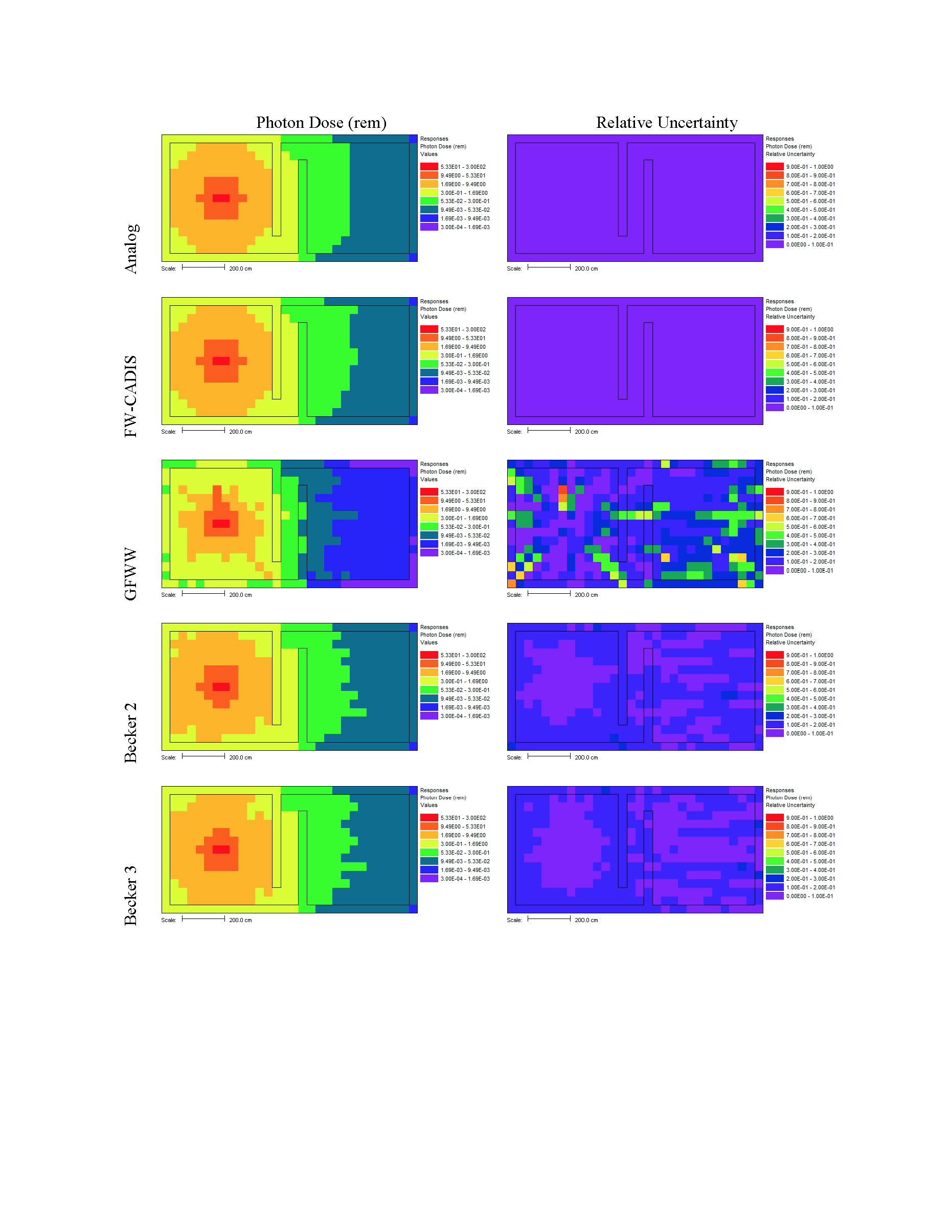
Fig. 4.4.3 Mesh tally results for the photon dose over the entire building use five different methods.
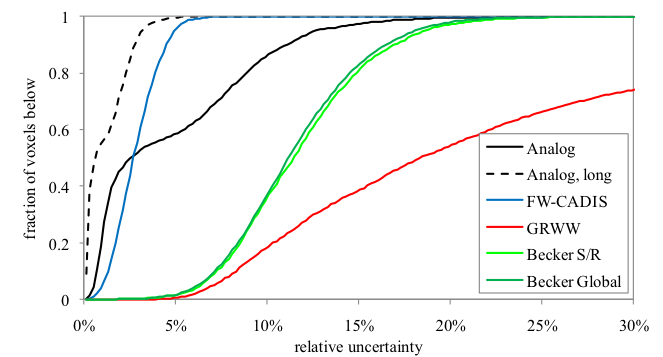
Fig. 4.4.4 The fraction of mesh tally voxels with less than a given amount of relative uncertainty for the five different methods.
Calculation method |
Forward SN (min) |
Adjoint SN (min) |
Monte Carlo (min) |
fraction of voxels with relative uncertainties less than 5% |
fraction of voxels with relative uncertainties less than 10% |
fraction of voxels with relative uncertainties less than 15% |
Analog |
20.1 |
0.583 |
0.857 |
0.973 |
||
Analog, long |
308.1 |
0.996 |
1.000 |
1.000 |
||
FW-CADIS, response weighting |
3.5 |
3.4 |
20.3 |
0.946 |
1.000 |
1.000 |
GRWW |
4.0 |
20.2 |
0.005 |
0.180 |
0.387 |
|
Becker, source/region |
4.0 |
3.6 |
19.0 |
0.016 |
0.350 |
0.800 |
Becker, global response |
4.2 |
4.4 |
20.4 |
0.016 |
0.358 |
0.832 |
4.4.3.4. Other special options for the importance map block input
In MAVRIC, the above methods have been extended to use biased sources. To turn off the use of a biased source, use the keyword “selfNormalize”. For forward flux-based methods, this will scale the target weights in the importance map so that the largest value is 1, which typically is at the source location. To use the forward-based Michigan methods (Cooper, GFWW, GRWW) or the van Wijk [MAV-AppC-VWVdEH11] methods as they were presented (without the MAVRIC biased source), use this keyword.
Use the keyword “spaceOnly=\(n\)” to create an importance map that contains one energy group over the entire range of energy. Use a value of 1 for neutron problems or a value of 2 for photon problems. This option is not designed for coupled problems. Both of the methods that van Wijk presents use importance maps that are space only.
Use the keyword “forwardParam=\(p\)” to allow the target weights to be proportional to the forward estimate (using Denovo) of flux raised to any power \(p\).
For Cooper’s method or van Wijk’s first method, \(p = 1\), which is the default if “forwardParam” is not specified. For van Wijk’s second method, based on the relative error estimate \(\text{Re}\left( \overrightarrow{r} \right) \propto \frac{1}{\sqrt{\phi\left( \overrightarrow{r} \right)}}\), set this parameter to \(p = 0.5\). Note that with a power less than 1, the weight window targets will span a smaller range than the expected Monte Carlo flux values. Particles may be rouletted before they reach the lowest flux areas of the problem.
When applying FW-CADIS for a semi-global problem, the adjoint source should cover the area where the lowest uncertainties are desired. Sometimes the area where this is desired is not a fixed geometric area but instead an area that has a final answer of a certain range. For example, when finding dose rate maps, the user may only be interested in getting low uncertainties for areas below the dose limit — areas above the dose limit may not matter as much since people will not be allowed in those areas. Another example may be that the dose map should be optimized in those areas above the background dose rate, since dose rates below that are of no concern. To allow the adjoint source area to be tailored in this way, the keywords “minForwardValue=” and/or “maxForwardValue=”can be used. Default values are 0 and 10100, respectively. For flux weighting, only the voxels within the adjoint source bounding box and containing a forward flux estimate between the min and max are included as adjoint sources.
A comparison [MAV-AppC-Pep13] of FW-CADIS to the University of Michigan methods and the Van Wijk methods showed that FW-CADIS performs better and is more straightforward to use than the other methods. These other methods were added to SCALE so that a fair comparison could be made and have been left in the code base for academic use in case some types of problems could benefit from them.
4.4.4. Using MAVRIC to run fixed-source Denovo calculations
The MAVRIC sequence of SCALE can be used to run the new discrete-ordinates code Denovo [MAV-AppC-ESSC10] The sequence is designed to use Denovo to compute an importance map for the Monte Carlo code Monaco but can be stopped without starting the final Monaco calculation. The full version of Denovo has a python-based user interface where the user must construct the geometry, source, and cross sections on their own. MAVRIC provides an easy interface to run the serial-only version of Denovo within SCALE (called ‘xkba’). Denovo inputs made using MAVRIC can also be imported into the python interface for the HPC version of Denovo.
To create Denovo inputs or run Denovo using MAVRIC, input the
composition, geometry (including arrays if needed), definitions (grid
geometry and response information), and sources block as if an actual
full MAVRIC case were being run. The sequence should then be started
with a parm=xxx flag to indicate to MAVRIC to stop after making Denovo
inputs or running Denovo.
parm= |
MAVRIC stops after |
|---|---|
Forward Calculations |
|
forinp |
Making cross sections and Denovo input |
forward |
Running Denovo |
Adjoint Calculations |
|
adjinp |
Making cross sections and Denovo input |
adjoint |
Running Denovo |
For forward Denovo simulations, the importance map block should contain which grid geometry to use and any of the optional Denovo parameters:
For forward Denovo simulations, the importance map block should contain which grid geometry to use and any of the optional Denovo parameters:
read importanceMap
    gridGeometryID=7
end importanceMap
For adjoint Denovo calculations, the importance map block should contain which grid geometry to use, one or more adjoint sources, and any of the optional Denovo parameters:
read importanceMap
    gridGeometryID=7
    adjointSource 1
        locationID=1
        responseID=5
    end adjointSource
end importanceMap
For either forward or adjoint, the following files will be produced and should be copied out of the SCALE temporary directory back to your home area:
ft02f001 |
the AMPX mixed working library cross section file |
|---|---|
xkba_b.inp |
binary input file for Denovo |
*.dff |
Denovo flux file (binary) - scalar fluxes |
The scalar flux file is automatically copied back to the home area when SCALE completes. The others can be copied back if desired using a shell command at the end of the MAVRIC input file:
=shell
    cp ft02f001   ${OUTDIR}/mixed.ft02f001
    cp xkba_b.inp ${OUTDIR}/denovo.dsi
end
The xkba_b.inp file and the *.dff file can both be viewed with the Java utility, Mesh File Viewer, that is shipped with SCALE. The xkba_b.inp file shows the Denovo source distribution (space and energy), and the *.dff shows the final computed scalar fluxes. The binary Denovo input file should be renamed with an extension of *.dsi (Denovo simple input) so that the viewer can properly interpret the data.
4.4.4.1. Optional Denovo parameters
The default values for various calculational parameters and settings used by Denovo for the MAVRIC sequence should cover most applications. These settings can be changed by the interested user in the importance map block. The two most basic parameters are the quadrature set used for the discrete ordinates and the order of the Legendre polynomials used in describing the angular scattering. The default quadrature order that MAVRIC uses is S8, and for the order of Legendre polynomials, the default is P3 (or the maximum number of coefficients contained in the cross section library, if less than 3). S8/P 3 should be a good choice for many applications, but the user is free to changes these. For complex ducts or transport over large distance at small angles, S12 may be required. S4/P 1 would be useful in doing a very cursory run just to check if the problem was input correctly. Other parameters that can be set by the user in the importance map block for Denovo calculations are listed in Table 4.4.4.

|
In problems with small sources or media that are not highly scattering, discrete ordinates can suffer from “ray effects”-where artifacts of the quadrature directions can be seen in the computed fluxes. To help alleviate the ray effects problem, Denovo has a first-collision capability. This computes the amount of uncollided flux in each mesh cell from a point source. These uncollided fluxes are then used as a distributed source in the main discrete-ordinates solution. At the end of the main calculation, the uncollided fluxes are added to the fluxes computed with the first-collision source, forming the total flux. While this helps reduce ray effects in many problems, the first-collision capability can take a long time to compute on a mesh with many cells or for many point sources.
The macromaterials option (“mmTolerance=”) can be used to better represent the geometry in Denovo. Refer to the main MAVRIC manual for details on macromaterials.
4.4.4.2. Forward source preparations
The user-entered source description is converted to a mesh-based source for Denovo. To create the mesh source, MAVRIC determines if the defined source exists within each cell. This is done by dividing each mesh cell into n\(\times\)n\(\times\)n subcells (from the keyword “subCells=n” in the importance map block with a default of n=2) and testing each subcell center. For every subcell center that is a valid source position (within the spatial solid and meets optional unit, region, or mixture requirements), an amount of source proportional to the subcell volume is assigned to the mesh cell. The keyword “subCells=” can be used to better refine how much source is computed for the mesh cells at the boundary of a curved source region. Of course, more subcell testing takes more time.
The above process may miss small sources or degenerate sources (surfaces, lines, points) that do not lie on the tested subcell centers. If none of the mesh cells contain any source after the subcell method, then random sampling of the source is used. A number of source positions are sampled from the source (set by the “sourceTrials=” keyword, default of 1000000) and then placed into the proper mesh cell. If this method is used, the resulting Denovo input file should be visualized to ensure that the statistical nature of the source trials method does not unduly influence the overall mesh source.
For forward calculations, if the number of mesh cells containing the true source is less than 10, then MAVRIC will convert these source voxels to point sources, to allow Denovo to use its first-collision capability to help reduce ray effects. The user can easily override the MAVRIC defaults-to force the calculation of a first-collision source no matter how many voxels contain source-by using the keyword “firstCollision.” To prevent the calculation of a first-collision source, the keyword “noFirstCollision” can be used.
For coupled problems, there are two ways to make Denovo compute photon fluxes from a neutron source: 1) include a tally using a photon response or 2) manually specify the “startGroup=” and the “endGroup=” to cover the particles/energy groups that are desired in the final Denovo output.
4.4.4.3. Adjoint source preparation
For adjoint calculations, adjoint sources that use point locations will use the Denovo first-collision capability. Volumetric adjoint sources (that use a boundingBox) will be treated without the first-collision capability. The keywords “firstCollision” and “noFirstCollision” will be ignored by MAVRIC for adjoint calculations.
Note that for an adjoint Denovo calculation, the MAVRIC input must still list a forward source. Otherwise, the sequence will report an error and stop. The forward source is not used for an adjoint Denovo calculation, but it must be present to make a legal MAVRIC input. For a coupled problem using an adjoint photon source, using a neutron forward source will make Denovo compute both photon and neutron adjoint fluxes. If the forward source(s) and adjoint source(s) are all photon, then only photon adjoint fluxes will be computed. The keywords “startGroup=” and “endGroup=” can also be used to manually set the particles/energy groups that are desired in the final Denovo output.
4.4.4.4. Other notes
Denovo (in SCALE 6) is a fixed-source SN solver and cannot model multiplying media. Neither forward nor adjoint neutron calculations from Denovo will be accurate when neutron multiplication is a major source component. If neutron multiplication is not turned off in the parameters block of the MAVRIC input (using keyword “noFissions”), a warning will be generated to remind the user of this limitation.
By default, MAVRIC instructs Denovo not to perform outer iterations for neutron problems if the cross-section library contains upscatter groups. This is because the time required to calculate the fluxes using upscatter can be significantly longer than without. For problems where thermal neutrons are an important part of the transport or tallies, the user should specify the keyword “upScatter=1” in the importance map block. This will instruct Denovo to perform the outer iterations for the upscatter groups, giving more accurate results but taking a longer time.
4.4.4.5. MAVRIC utilities for Denovo
Denovo simply calculates scalar fluxes for every mesh cell and energy group — it does not compute responses based on those fluxes. Several utilities have been added to the collection of MAVRIC utilities in order to allow the user to further process Denovo scalar flux results. The full details and input descriptions for these utilities can be found in the MAVRIC Utilities description in Sect. 4.3.
dff2dso |
Convert a Denovo flux file into a Denovo spatial output file. |
dff2mai |
Convert a Denovo flux file into a mesh angular information file. |
dff2mim |
Invert a Denovo flux file and store as a mesh importance map. |
dff2msl |
Convert a Denovo flux file into a mesh source lite. |
dffBinOp |
Binary operation of Denovo flux files: sum, difference, product, and ratio. |
dffDisp |
Display the basics of a Denovo flux file. |
dffFilter |
Perform various filters on a Denovo flux file. |
dffFix |
Fix the zero and negative values in a Denovo flux file. |
dffInt |
Integrate a single particle type from a Denovo flux file. |
dffInv |
Invert the values in a Denovo flux file. |
dffMult |
Multiply a Denovo flux file by a constant factor. |
dffPull |
Pull fluxes from certain voxels out of a Denovo flux file. |
dffResp |
Apply a response function to scalar fluxes in a Denovo flux file. |
dffSplit |
Split off a single particle type from a Denovo flux file. |
There are also two utility programs that look at the Denovo simple input file (binary) that MAVRIC creates. In the SCALE temporary directory, the file is called xkba_b.inp. In order to display in the MeshFileViewer, Denovo simple input files need to be renamed with a *.dsi extension. The utilities are as follows.
dsi2asc |
Convert a Denovo simple input (*.dsi) from binary to ASCII (so the user can see every detail). |
dsiDisp |
Display the basics of a Denovo simple input file. |
4.4.4.6. Example problem
4.4.4.6.1. Forward
As an example, consider a simulation based on the Ueki shielding experiments (see Monaco manual). A 252Cf neutron source was placed in the center of a 50 cm cube of paraffin which had a 45\(^{\circ}\) cone cut-out. The goal is to calculate the neutron dose at a detector 110 cm from the source.
The input file (denovo1.inp) needs the compositions of the paraffin and
graphite
read composition
    para(h2o)    3         1.0 293.0 end
    carbon       4 den=1.7 1.0 293.0 end
end composition
then the geometry
read geometry
    global unit 1
        cuboid  1   25.0 -25.0  25.0 -25.0   25.0 -25.0
        cone    2  10.35948  25.01   0.0 0.0   rotate  a1=-90 a2=-90 a3=0
        cuboid  3   90.0  70.0  40.0 -40.0   40.0 -40.0
        cuboid 99  120.0 -30.0  50.0 -50.0   50.0 -50.0
        media 3 1  1 -2
        media 0 1  2
        media 4 1  3
        media 0 1  99 -1  -2 -3
    boundary 99
end geometry
then the position of the detector, the response of the detector and the mesh to use for Denovo
read definitions
    location 1
        position 110 0 0
    end location
    response 5
        title="ANSI standard (1977) neutron flux-to-dose-rate factors"
        specialDose=9029
    end response
    distribution 1
        title="Cf-252 neutrons, Watt spectrum a=1.025 MeV and b=2.926/MeV"
        special="wattSpectrum"
        parameters 1.025 2.926 end
    end distribution
    gridGeometry 7
        xLinear 4 -25 -5
        xLinear 15 -5 25
        xLinear  9 25 70
        xLinear  8 70 90
        xplanes -30 95 100 105 109 111 115 120  end

        yplanes -50 -40 40 50 end
        yLinear  5 -40 -15
        yLinear 15 -15 15
        yLinear  5  15 40

        zplanes -50 -40 40 50 end
        zLinear  5 -40 -15
        zLinear 15 -15 15
        zLinear  5  15 40
    end gridGeometry
end definitions
the description of the true source
read sources
    src 1
        neutrons  strength=4.05E+07
        cuboid  0.01 0.01  0 0  0 0
        eDistributionID=1
    end src
end sources
and finally the importance map block to trigger the Denovo calculation
read importanceMap
    gridGeometryID=7
    macromaterial
      mmTolerance=0.001
    end macromaterial
end importanceMap
An optional shell command can be used to retrieve the cross section file and the Denovo input file.
=shell
  cp ft02f001       ${OUTDIR}/denovo1.ft02f001
  cp xkba_b.inp     ${OUTDIR}/denovo1.xkba.dsi
end
The denovo1.xkba.dsi file (the Denovo simple input) contains both the source and mesh
geometry that MAVRIC prepared for Denovo, as shown in Fig. 4.4.5.
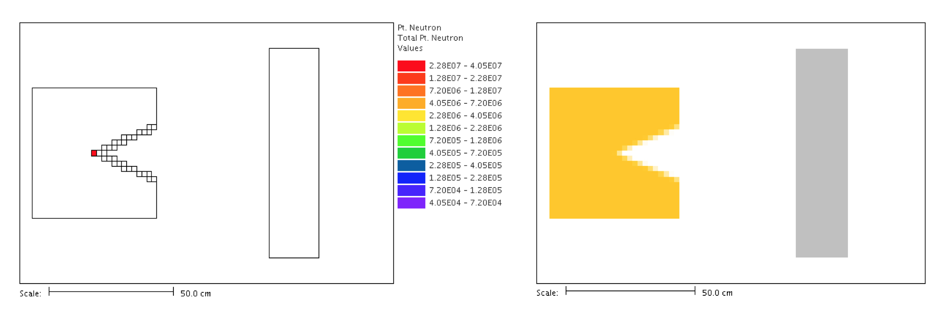
Fig. 4.4.5 Forward Denovo source (left) and mesh geometry (right).
The result of the Denovo-only MAVRIC calculation is a file,
denovo1.forward.dff, containing the scalar fluxes for each energy group.
The Mesh File Viewer can be used to display each group or the total scalar flux, which is shown in Fig. 4.4.6.
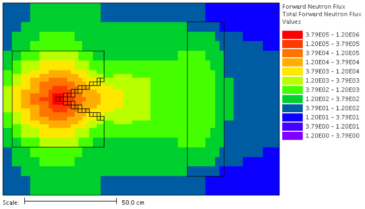
Fig. 4.4.6 Total forward fluxes.
The MAVRIC utilities can be used to further process the Denovo flux into a detector response. The fluxes at the location of the detector need to be multiplied by the photon flux-to-dose conversion factors (the response function) and then summed. This is can be done in the same input file using
=dffResp
"denovo1.forward.dff"
1
27
1.6151395E-04
1.4451494E-04
1.2703618E-04
1.2810882E-04
1.2983654E-04
1.0343020E-04
5.2655141E-05
1.2860853E-05
3.7358122E-06
3.7197628E-06
4.0085556E-06
4.2945048E-06
4.4731187E-06
4.5656334E-06
4.5597271E-06
4.5209654E-06
4.4872718E-06
4.4659614E-06
4.4342228E-06
4.3315831E-06
4.2027596E-06
4.0974155E-06
3.8398102E-06
3.6748431E-06
3.6748440E-06
3.6748431E-06
3.6748447E-06
"denovo1.doses.dff"
end

=dffInt
" denovo1.doses.dff"
1
" denovo1.total.dff"
end

=dffPull
" denovo1.total.dff"
1
110.0 0.0 0.0
0
"denovo1.detectorDose.txt"
end
and results in a neutron dose rate of 5.426 \(\times\) 10-3 rem/hr, calculated in about 2 minutes. Other combinations of the MAVRIC utilities can be used to simply “pull” out the fluxes from the detector location and then use a spreadsheet to compute the dose rate. With upscatter on, the result is 5.424 \(\times\) 10-3 rem/hr, showing that upscatter does not contribute to dose rate at the detector. Note that with upscatter on, the Denovo calculation required 81 minutes.
4.4.4.6.2. Adjoint
For the same calculation of neutron dose as above, a Denovo adjoint
calculation can be performed. The input file (denovo2.inp) has the same
composition, geometry, definitions, and source blocks as the forward
example. The adjoint input importance map block contains a description
of the adjoint source:
read importanceMap
    adjointSource 1
        locationID=1
        responseID=5
    end adjointSource
    gridGeometryID=7
    macromaterial
      mmTolerance=0.001
    end macromaterial
end importanceMap
The result of this Denovo-only MAVRIC calculation is a file,
denovo2.adjoint.dff, containing the scalar adjoint fluxes for each
energy group, as shown in Fig. 4.4.7.
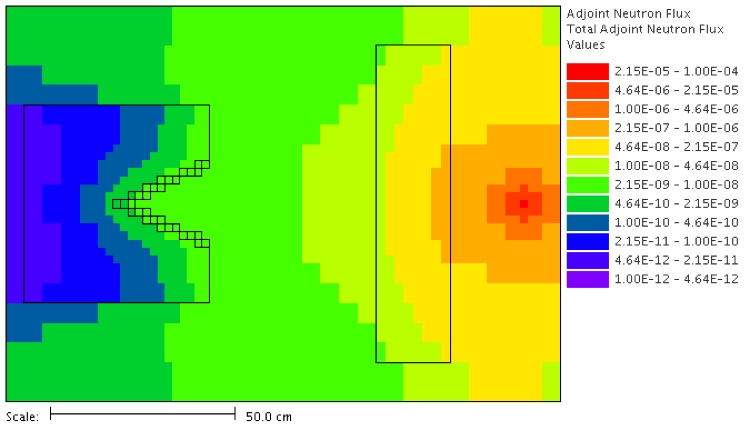
Fig. 4.4.7 Total adjoint fluxes.
As with the forward fluxes, the MAVRIC utilities can be used to further process the Denovo adjoint fluxes into a detector response. The adjoint fluxes at the location of the forward source need to be multiplied by the source distribution and strength and then summed. This is can be done using
=dffResp
"denovo2.adjoint.dff"
1
27
3.365455E-02
2.398546E-01
2.398289E-01
1.085244E-01
1.527957E-01
1.463752E-01
6.669337E-02
1.164470E-02
5.713197E-04
5.240384E-05
4.470401E-06
2.956226E-07
4.160008E-08
1.011605E-08
9.667897E-10
3.579175E-10
9.880883E-11
6.634570E-11
9.742191E-11
1.538334E-10
2.777230E-11
2.690255E-11
2.572180E-11
7.001169E-12
2.049478E-12
1.437105E-12
3.424200E-13
"denovo2.doses.dff"
end

=dffMult
" denovo2.doses.dff"
4.05E+07
" denovo2.doses.dff"
end

=dffInt
" denovo2.doses.dff"
1
" denovo2.total.dff"
end


=dffPull
" denovo2.total.dff"
1
0.0 0.0 0.0
0
"denovo2.detectorDose.txt"
end
and results in a neutron dose rate of \(5.463 \cdot 10^{-3}\) rem/hr.
The results of the example problems above used a fairly coarse mesh (44 \(\times\) 27 \(\times\) 27) and the default values of S8 and P3. Run times were 2 minutes for the forward case and 2.5 minutes for the adjoint. With a finer mesh, larger quadrature order and larger numbers of Legendre moments for the scattering representation, the values calculated using Denovo should converge towards the Monte Carlo solution of \(1.494 \cdot 10^{-2}\ \text{rem/hr} \pm 1.2\%\).
References
- MAV-AppC-Bec09
T. L. Becker. Hybrid Monte Carlo/Deterministic Methods for Deep-Penetration Problems. PhD Thesis, University of Michigan, 2009.
- MAV-AppC-BL09
T. L. Becker and E. W. Larsen. The application of weight windows to ‘global’monte carlo problems. In Proc. Conf. Advances in Mathematics, Computational Methods, and Reactor Physics. American Nuclear Society Saratoga Springs, New York, 2009.
- MAV-AppC-CL01
Marc A. Cooper and Edward W. Larsen. Automated weight windows for global Monte Carlo particle transport calculations. Nuclear Science and Engineering, 137(1):1–13, 2001. Publisher: Taylor & Francis.
- MAV-AppC-ESSC10
Thomas M. Evans, Alissa S. Stafford, Rachel N. Slaybaugh, and Kevin T. Clarno. Denovo: A new three-dimensional parallel discrete ordinates code in SCALE. Nuclear technology, 171(2):171–200, 2010.
- MAV-AppC-Pep13(1,2)
Douglas E. Peplow. Comparison of hybrid methods for global variance reduction in shielding calculations. In Proceedings of the 2013 International Conference on Mathematics and Computational Methods Applied to Nuclear Science and Engineering-M and C 2013. 2013.
- MAV-AppC-PME12
Douglas E. Peplow, Scott W. Mosher, and Thomas M. Evans. Consistent Adjoint Driven Importance Sampling Using Space, Energy and Angle. Technical Report ORNL/TM-2012/7, Oak Ridge National Laboratory, Oak Ridge, TN (USA), 2012.
- MAV-AppC-PMEW10
Douglas E. Peplow, Scott W. Mosher, Thomas M. Evans, and J. C. Wagner. Hybrid Monte Carlo/Deterministic Methods for Streaming/Beam Problems. In American Nuclear Society Radiation Protection and Shielding Division 2010 Topical Meeting, Las Vegas, Nevada. 2010.
- MAV-AppC-VRUS97
K. A. Van Riper, T. J. Urbatsch, and P. D. Soran. AVATAR – Automatic variance reduction in Monte Carlo calculations. Technical Report LA-UR-97-919; CONF-971005-10, Los Alamos National Laboratory, Los Alamos, NM (USA), May 1997. URL: https://www.osti.gov/biblio/527548 (visited on 2020-08-11).
- MAV-AppC-VWVdEH11
A. J. Van Wijk, Gert Van den Eynde, and J. E. Hoogenboom. An easy to implement global variance reduction procedure for MCNP. Annals of Nuclear Energy, 38(11):2496–2503, 2011. Publisher: Elsevier.