4.2. MAVRIC CAAS Capability
4.2.1. Introduction
Modeling criticality accident alarm systems (CAAS) presents challenges since the analysis consists of both a criticality problem and a deep-penetration shielding problem [CAASPLMP10, CAASPPJ09]. Modern codes are typically optimized to handle one of those types of problems but usually not both. The two problems also differ in scale-the criticality problem depends on materials relatively close to the fissionable materials while the shielding problem can cover a much larger range. SCALE now contains fully three-dimensional tools to perform both parts of a CAAS analysis.
CAAS analysis can be performed with SCALE using the KENO-VI criticality code and the MAVRIC shielding sequence. First, the fission distribution (in space and energy) is determined by KENO-VI. This distribution is saved to a file using a user-specified three-dimensional mesh grid and an energy structure from the cross section library (or a user-defined energy structure). MAVRIC then uses the fission distribution as the source for a shielding calculation. MAVRIC is designed to implement advanced variance reduction methods to calculate dose rates or detector responses for difficult shielding problems.
For different types of shielding and different combinations of sources and detector locations, different strategies can be used within SCALE [CAASPW12, CAASWODonnellN12]. Due to the way that cross sections for neutron reactions that create photons are stored in ENDF, some of the parameters used in the CAAS capability have changed since SCALE 6.1. Please be sure to understand and follow the new guidance for the correct accounting of secondary photons from neutron reactions [CAASMP13a, CAASMP13b, CAASMP13c].
4.2.2. Methods
The CAAS capability in SCALE is a two-step approach using KENO-VI and MAVRIC. The first step is the determination of the source distribution, done with the CSAS6 sequence which uses the KENO-VI functional module. Along with calculating the system keff, KENO-VI has been modified to now accumulate the fission distribution over the non-skip generations. This information is collected on a three-dimensional Cartesian mesh that overlays the physical geometry model and is saved as a Monaco mesh tally file. A utility program is used to convert the mesh tally into a Monaco mesh source.
The mesh source is then used in the second step as the source term in MAVRIC. The absolute source strength is set by the user based on the total number of fissions (based on the total power released) during the criticality excursion. Further neutron multiplication should be prevented in the MAVRIC transport calculation. Because the fission neutrons have already been accounted for in the KENO-VI calculation, failure to suppress neutron multiplication in the MARVIC sequence would lead to incorrect flux estimates. In addition, if further fissions were allowed, Monaco would add neutrons to its particle bank faster than they could be removed (since the system is at or above critical) and the simulation may never finish.
For the transport part of a CAAS analysis, MAVRIC can be optimized to calculate one specific detector response at one location using CADIS or can be optimized to calculate multiple responses/locations with roughly the same relative uncertainty using FW-CADIS. For calculating mesh tallies of fluxes or dose rates, MAVRIC also uses FW-CADIS to help balance the Monaco Monte Carlo calculation such that low flux voxels are computed with about the same relative uncertainty as high flux voxels.
With this two-step approach, users will have a great deal of flexibility in modeling CAAS problems. The CSAS6 step and the MAVRIC step could both use the same geometry and materials definitions or could have different levels of detail included in each. The fission source distribution from one CSAS6 calculation could be used in a number of different MAVRIC building/detector models, with each MAVRIC calculation being optimized for a given type of detector.
4.2.3. User Input
The user can create either one input file containing both the CSAS6 and MAVRIC calculations or can create two input files-one for each sequence. The materials and geometry for these two models could be the same but do not have to be. For example, the CSAS6 sequence might only contain the materials and geometry important to the criticality calculation. Note, however, that the critical source geometry and materials should be modeled identically in both problems. This allows users greater flexibility in modeling their specific problems.
4.2.3.1. KENO-VI input
For the criticality problem, the only extra input a user needs to supply is the keyword cds=yes in the parameter block and a spatial mesh around all of the fissionable materials of the problem in its own gridGeometry block. Standard input for KENO-VI is described in the KENO-VI chapter and CSAS6 chapter. The mesh used for the fission source distribution is input using the read gridGeometry *id* block, where id is an identification number for that grid. Note that only one grid can be specified, but that may change in the future. The cells of the mesh are specified in each dimension separately by either (1) listing all of the planes bounding the cells (keyword “xplanes” followed by an “end”), (2) using keyword xLinear *n* *a* *b* to specify n cells between a and b, or by (3) specifying the minimum plane, the maximum plane, and how many cells to make in that dimension (xmin=, xmax=, numXCells=). The keywords xplanes and xLinear can be used together and multiple times. Similar keywords are used for the y- and z-dimensions. An example CSAS6 input file that collects the fission distribution information would be as follows:
=csas6
CAAS Example
v7-238n
read composition
    …
end composition
read parameters
    …
    cds=yes
end parameters
read geometry
    …
end geometry
read gridGeometry 1
    title="Mesh for Collecting Fission Source"
    xLinear 13 0.0 78.0
    yplanes 0 8 16 24 32 34 36 38 40 48 56 64 72 end
    zLinear 10 -2.54 77.46
end gridGeometry
end data
end
The fission source distribution collected by KENO-VI is saved to a Monaco mesh tally file and copied back to the home area with the name *problemName*.fissionSource.3dmap. This file can be viewed with the Mesh File Viewer capability of Fulcrum that comes with SCALE. Note that the finer the mesh spacing is the more generations/histories will have to be simulated by the criticality calculation in order to reduce the stochastic uncertainty in each mesh voxel of the distribution. Regardless of the mesh size, creation of a fission mesh source file will take more iterations than the number required to find keff. KENO-VI also saves the value of the system the average number of neutrons per fission, in a file called *problemName*.kenoNuBar.txt. This value is needed to properly determine the source strength.
4.2.3.2. Mesh tally to mesh source conversion
A utility program is used to convert the Monaco mesh tally file into a Monaco mesh source file. It can be part of the CSAS6 input file. The user then needs to copy the resulting *.msm file back to his home area.
=csas6
…
end

=mt2msm
'fissionSource.3dmap'    ! existing Keno fission source mesh tally
1                        ! which family (for Keno files, there is only 1)
-1                       ! use the whole family (keep all energy groups)
1                        ! particle type for *.msm file (1-neutron, 2-photon)
'fissionSource.msm'      ! name of newly created mesh source map file
end

=shell
  copy fissionSource.msm "C:\mydocu~1\caasExample"
end
Details on the conversion utility program are contained in Sect. 4.3 of the MAVRIC manual.
In SCALE 6.1, the fission source distribution mesh tally produced by KENO contained data representing the number of fissions in each mesh cell in each energy group. In SCALE 6.2, the data stored was changed to be the fissions per unit volume - the fission density. This is more consistent with other mesh tallies from Monaco which store flux or dose rates that represent averages over the mesh cells. This change also allows the Mesh File Viewer to display the KENO fission source distribution better. The mt2msm utility program also changed from SCALE 6.1 to SCALE 6.2 to account for the change in what is stored in the Keno mesh tally file. Therefore, KENO-produced fission source mesh tallies and the mt2msm utility should not be mixed-and-matched across versions of SCALE. Doing so would result in the final Monaco mesh source file being improperly normalized, which would not represent the KENO fission source distribution and would give incorrect results in subsequent MAVRIC calculations. Because there is not a specific ‘version flag’ in a mesh tally file or mesh source map file, the user must ensure that they have used the same version of SCALE for both the CSAS6 and MAVRIC sequences any time the CAAS capability is used.
4.2.3.3. MAVRIC input
The input for the MAVRIC portion of the CAAS problem should include the materials and geometry of the criticality model, use the fission distribution as a source, set the source strength, and set any optional modifiers to the source to change its location or add fission photons. The cross section library used by the MAVRIC calculation does not need to have the same group structure as the fission distribution. MAVRIC will automatically convert the fission source group structure to match the group structure of its cross section library.
The shielding calculation needs to specify that the source is the fission distribution file, which is typically fissionSource.msm. The total source strength can be specified by either the number of fissions in the criticality accident (fission rate or total number) or by the number of released neutrons (the fission rate multiplied by \(\over{v}\) per fission). The value of \(\over{v}\) will be read from the file kenoNuBar.txt in the SCALE temporary directory if it is not given in the source input with the keyword nu-bar=. The mesh source can also be placed at different coordinates in the geometry using the origin x= *x* y= *y* z=*z* keywords, if a different reference frame was used with the criticality geometry model that created the mesh source. Rotations of mesh sources are not available at this time. It is also recommended to use filters in the source block to define the source, such as the mixture= filter to only allow source sampling from a specific mixture since the mesh source can be transformed from its original origin or meshes can cover non-fissionable materials.
For example, using a KENO-VI fission distribution, placing it somewhere in the MAVRIC model and setting the source strength (in neutrons/s) to correspond to 1017 fission/s would look like
=shell
    copy "C:\mydocu~1\caasExample\kenoInput.kenoNuBar.txt"  kenoNuBar.txt
end

=mavric
…
read sources
    src 1
        meshSourceFile "C:\mydocu~1\caasExample\fissionSource.msm"
            origin x=600 y=650 z=400
        fissions=1.0e17
    end src
end sources
…
end data
end
The source strength in neutrons/s will be calculated by MAVRIC to be the fission rate multiplied by the value of read from the “kenoNuBar.txt” file. The neutron strength could have alternatively been specified using the standard source strength keyword “strength=2.5e17” (for an example with the average number of neutrons per fission of 2.5).
The Monte Carlo functional module used by MAVRIC, Monaco, is a fixed-source code. Unless told otherwise, neutrons will multiply in fissionable materials. Since all of the neutrons were part of the source, neutron multiplication should not be allowed and MAVRIC should be run with the keyword “fissionMult=0” in the parameters block. For systems at or near critical without the “fissionMult=0” keyword, Monaco simulations may not end since neutrons will be added to the particle bank at the same rate they leave the system or get killed.
The shielding calculation can be run using standard variance reduction methods (such as path length stretching, user-defined weight windows based on geometry regions, and user-defined source biasing) or using the automated tools which employ approximate discrete-ordinates calculations to determine the space/energy weight windows as well as a biased source distribution in space and energy. The automated tools can be used to optimize the shielding calculation to determine one specific tally using CADIS or several separate tallies or a mesh tally over a large volume of the problem space using FW-CADIS. When using these advanced variance reduction methods, remember to include planes in the discrete-ordinates mesh definition that correspond to the planes in the fission distribution that the source is based on. If they are not included, MAVRIC will resample the fission source on the discrete-ordinates mesh it is using for the importance map, possibly smearing or reducing the original resolution of the fission distribution.
4.2.4. Example problem
Consider the Jezebel critical plutonium sphere experiment, shown in Fig. 4.2.1, taking place inside a simple fictitious building, shown in Fig. 4.2.2. The building has two rooms: an experiment room and a control room. In the control room there is a criticality alarm detector, and it is positioned furthest from the entry to the experiment room. For this example, assume that a criticality excursion results in a total of 1018 fissions. This example will calculate the neutron and photon doses seen by a detector in the control room, as well as calculate a dose map for the entire building.
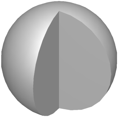
Fig. 4.2.1 Cutaway view of Jezebel.
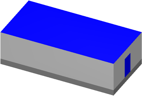
Fig. 4.2.2 Simple two-room building.
4.2.4.1. KENO-VI criticality and fission source distribution
For the criticality calculation, consider just a bare sphere of
plutonium, with a radius of 6.38493 cm. Atom densities (atoms/b\(\cdot\)Pu 0.037047; 240Pu
0.0017512; 241Pu 0.00011674; and Cu 0.0013752. This can be
easily modeled as a sphere at the origin. For collecting the fission
distribution, a uniform mesh grid can be constructed around the sphere,
extending 7 cm in each direction, with a 1 \(\times\) 1 \(\times\) 1 cm voxel size. The first
portion of the input files mavric.caasA.inp and mavric.caasB.inp looks
like the following:
=csas6
Dose Rates from a Jezebel Accident in a Block Building
v7-238n
'-------------------------------------------------------------------------------
' Composition Block
'-------------------------------------------------------------------------------
read composition
    Pu-239 1 0 0.037047   end
    Pu-240 1 0 0.0017512  end
    Pu-241 1 0 0.00011674 end
    Cu     1 0 0.0013752  end
end composition

'-------------------------------------------------------------------------------
' Parameters Block
'-------------------------------------------------------------------------------
read parameters
    gen=250 npg=200000 nsk=50 htm=no
    cds=yes
end parameters
'-------------------------------------------------------------------------------
' Geometry Block - SCALE standard geometry package (SGGP)
'-------------------------------------------------------------------------------
read geometry
    global unit 2
        sphere 1  6.38493
        media 1 1 1 vol=1090.3277
    boundary 1
end geometry

'-------------------------------------------------------------------------------
' Grid Block
'-------------------------------------------------------------------------------
read gridGeometry 1
    title="Mesh for Collecting Fission Distribution"
    xLinear 14 -7.0 7.0
    yLinear 14 -7.0 7.0
    zLinear 14 -7.0 7.0
end gridGeometry

end data
end

=mt2msm
'fissionSource.3dmap'
1
-1
1
mavric.caas[A/B].fissionSource.msm'
end
The results of this 26 minute calculation are shown in Table 4.2.1, and details about the calculated fission distribution are shown in Fig. 4.2.3 and Fig. 4.2.4.
Quantity |
Value |
Uncertainty |
|
|---|---|---|---|
keff |
best estimate system k-eff |
1.00024 |
0.00014 |
\(\over{v}\) |
system nu bar |
3.15671 |
4.77938E-05 |

Fig. 4.2.3 Fission source spatial distribution for the center horizontal slice.
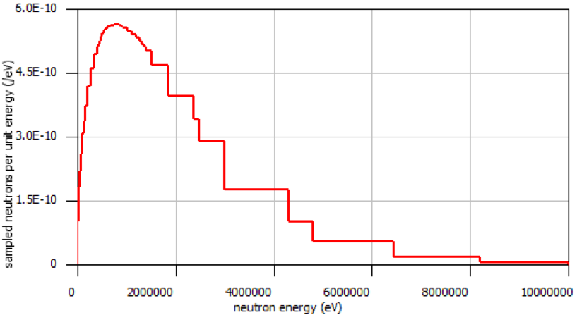
Fig. 4.2.4 Fission source energy distribution for the center voxel.
4.2.4.2. MAVRIC transport calculations
Two MAVRIC calculations will be done-one that calculates the doses seen at the detector and one that computes mesh tallies of doses over the entire building. They will share the same materials, geometry, and source but will have different tally and variance reduction options.
The two-room building will be a simple model using concrete-block walls, a concrete floor, and a steel roof, with dimensions shown in Fig. 4.2.5. The building exterior dimensions are 1200 cm long, 600 cm wide, and 300 cm high above the ground. The exterior and interior walls are all made of a double layer of typical concrete blocks (total of 40 cm thick.) Concrete blocks are typically 39 \(\times\) 19 \(\times\) 19 cm and weigh ~13.5 kg, since they have a volume fraction of 33.2%. The floor is made of poured concrete, extending 60 cm into the ground. The roof and the exterior door (120 cm wide and 210 cm tall) are made of 1/8 in. (0.3175 cm) thick steel. The experiment room on the left connects to the control room on the right through a maze that prevents radiation streaming. Assume that the critical experiment was in the center of the experiment room, 100 cm above the floor. Assume the detector in the control room is a 30 cm diameter sphere located at position (1145, 55, 285).
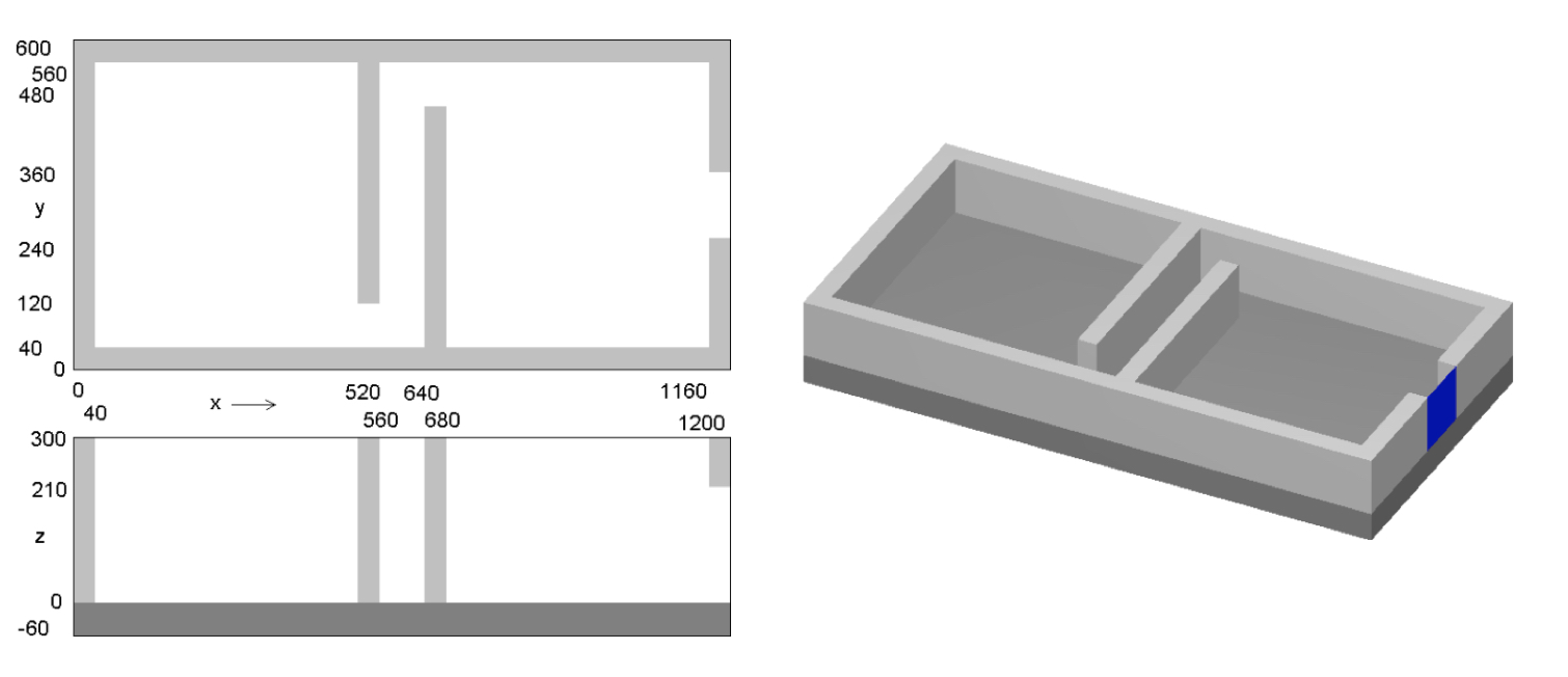
Fig. 4.2.5 Coordinates of the floor, walls, ceiling, and door of the simple block building model (in cm).
If the MAVRIC transport calculation is not in the same file as the CSAS6 calculation, the MAVRIC input would start by moving the KENO-VI results into the SCALE temporary area:
=shell
    copy %RTNDIR%\caas.kenovi.fissionSource.msm  fissionSource.msm
    copy %RTNDIR%\caas.kenovi.kenoNuBar.txt      kenoNuBar.txt
end
The materials and geometry blocks of the two MAVRIC input files for each of the two calculations,
smplprbs/caas.mavricA.inp and smplprbs/caas.mavricB.inp, look like the following:
'-------------------------------------------------------------------------------
' Composition Block
'-------------------------------------------------------------------------------
read composition
    pu-239 1 0 0.037047   end
    pu-240 1 0 0.0017512  end
    pu-241 1 0 0.00011674 end
    cu     1 0 0.0013752  end
    orconcrete 2 1.0     293.0 end
    orconcrete 3 0.33198 293.0 end
    ss304      4 1.0     293.0 end
end composition

'-------------------------------------------------------------------------------
' Geometry Block - SCALE standard geometry package (SGGP)
'-------------------------------------------------------------------------------
read geometry
    global unit 1
        com="jezebel"
        sphere   1  6.38493  origin x=280  y=300  z=100

        com="exterior of the building, roof, floor"
        cuboid   10 1200 0    600 0     300.3175 -60.0
        cuboid   11 1200 0    600 0     300.3175 300.0
        cuboid   12 1200 0    600 0     0.0        -60

        com="air space in building - two rooms and maze"
        cuboid   20 1160 40   560 40    300 0

        com="interior walls to form maze to prevent streaming"
        cuboid   21  560 520  560 120   300 0
        cuboid   22  680 640  480  40   300 0

        com="exterior door"
        cuboid   30 1200 1160       360 240   210 0
        cuboid   31 1200 1199.6825  360 240   210 0

        com="detector sphere"
        sphere  40   15.0  origin x=1145 y=55 z=285

        com="jezebel"
        media  1 1   1   vol=1090.3277

        com="walls, roof, floor"
        media  3 1   10 -20 -11 -12  -30
        media  4 1   11
        media  2 1   12

        com="air space (void) and maze walls"
        media  0 1   20 -21 -22   -40  -11 -12  -1
        media  3 1   21                -11 -12
        media  3 1   22                -11 -12

        com="exterior door"
        media  0 1   30 -31
        media  4 1   31

        com="detector"
        media  0 1   40   vol=14137.167

    boundary 10
end geometry
The response functions used to compute the doses will be the standard flux-to-dose rate conversion factors for neutrons and photons. These are defined in the definitions block. Note that these responses have units of (rem/hr)/(/cm 2/s).
'-------------------------------------------------------------------------------
' Definitions Block
'-------------------------------------------------------------------------------
read definitions
    response 5
        title="ANSI (1977) neutron flux-to-dose-rate"
        specialDose=9029
    end response
    response 6
        title="ANSI (1977) photon flux-to-dose-rate"
        specialDose=9504
    end response
end definitions
The source used by each MAVRIC simulation will be based on the fission distribution mesh source determined by KENO-VI. The strength of the source can be specified by the total number of fissions that occurred in the criticality event. Fission photons will be added for 239Pu. MAVRIC will determine the total source strength, including the fission photons, from the value of saved by KENO-VI and the multiplicity data from the fission photon data file.
'-------------------------------------------------------------------------------
' Sources Block
'-------------------------------------------------------------------------------
read sources
    src 1
        meshSourceFile="fissionSource.msm"
        origin x=280  y=300  z=100
        fissions=1.0e18
        mixture=1
    end src
end sources
Note that further multiplication needs to be turned off in MAVRIC using the fissionMult=0 keyword in the parameter block as shown below.
For the responses from the tallies, MAVRIC usually calculates dose rates (rem/hr) using a source strength in particles/s. For this example problem, instead of a source rate, we used a total number of particles (by specifying the number of fissions). Hence, the computed fluxes will have units of particles/cm2 and the computed responses using the standard dose responses from the cross section libraries will have units of rem s/hr. To get a dose in rem, the responses need to be multiplied by (3600 s/hr)-1. This can be done using the MAVRIC tally multiplier keyword.
Each MAVRIC simulation will need a discrete-ordinates mesh. The planes in each dimension where there are material changes are listed in Table 4.2.2. In addition to these planes, the discrete-ordinates mesh should also subdivide the thick shields in the direction of particle travel. For example, the walls of the maze should be divided to better model the radiation attenuation through the walls in the Denovo calculation. The interior walls of the building will reflect particles, so the first few centimeters are the most important to capture in the importance map. Mesh planes should also be added that correspond to the mesh source after it is placed into the geometry model.
x |
y |
z |
|---|---|---|
0 |
0 |
-60 |
40 |
40 |
0 |
520 |
120 |
210 |
560 |
240 |
300 |
640 |
360 |
300.318 |
680 |
480 |
|
1160 |
560 |
|
1199.68 |
600 |
|
1200 |
4.2.4.2.1. Detector doses using CADIS
The grid geometry for this calculation should also include planes that bound the adjoint source,
which is the detector area (these values are shown in brackets [] below). The definitions block in
smplprbs/caas.mavricA.inp also includes the location of the center of the detector, which is used in the adjoint source description.
location 1
     position 1145 55 285
 end location

 gridGeometry 1
     title="mesh for discrete ordinates 57 x 47 x 31 = 83049"
     xplanes 0     10 20 30 35
             40    120 160 240
                   270 272 274 276 278 280 282 284 286 288 290
                   360 440
             520   525 530 550 555
             560   600
             640   645 650 670 675
             680   760 840 920 1000 1080
                   [1130 1140 1150]
             1160  1165 1170 1180 1190
             1199.6825
             1200  end
     yplanes 0     10 20 30 35
             40    [50 60] 70
             120   125 130 140 200
             240   280 290 292 294 296 298 300 302 304 306 308 310
                   320
             360   440 460 470 475
             480
             560   565 570 580 590
             600   end
     zplanes -60   -30 -20 -10 -5
             0     45
                   90 92 94 96 98 100 102 104 106 108 110
                   140 175
             210   255  [280 290]
             300
             300.3175   end
 end gridGeometry
The tallies are region tallies over the detector region (the 10th media card in unit 1) using the appropriate response function for the particle type of the tally. The volume of the detector sphere needs to be listed in the geometry block so that the fluxes and tallies will be correctly computed. The importance map uses standard CADIS to bias the particles towards the detectors, optimizing the calculation of the total dose (by listing both response functions together, the total response will be used in the adjoint source).
'-------------------------------------------------------------------------------
' Tallies Block
'-------------------------------------------------------------------------------
read tallies
    regionTally 1
        title="Doses seen by the detector"
        neutron
        unit=1 region=10
        responseID=5
        multiplier=2.777778e-4
    end regionTally
    regionTally 2
        title="Doses seen by the detector"
        photon
        unit=1 region=10
        responseID=6
        multiplier=2.777778e-4
    end regionTally
end tallies

'-------------------------------------------------------------------------------
' Parameters Block - 3 min batch
'-------------------------------------------------------------------------------
read parameters
    randomSeed=3263827
    perBatch=654000  batches=40
    fissionMult=0
end parameters

'-------------------------------------------------------------------------------
' Importance Map Block
'-------------------------------------------------------------------------------
read importanceMap
    gridGeometryID=1
    adjointSource 1
        locationID=1
        responseIDs 5 6 end
    end adjointSource
end importanceMap
The results of this example problem are shown in Table 4.2.3. Calculation times were 12 minutes for Denovo and 135 minutes for Monaco. Note that the uncertainty for the photon dose is much higher than the neutron dose uncertainty. This is because the simulation was optimized for the calculation of total dose, and the photon component of the total dose is less than 2%. Had a separate calculation been done that used an adjoint source of just the photon response, the photon dose rate uncertainty would have been much smaller but at the expense of the neutron dose rate uncertainty. A single calculation could have also been performed using two adjoint sources, one using the neutron dose response and one using the photon dose response, and forward weighting to help calculate each component of dose with more uniform relative uncertainties.
Value |
Rel. |
|
|---|---|---|
Dose |
(rem) |
Unc. |
neutron |
1539 |
0.78% |
photon |
30.0 |
8.00% |
4.2.4.2.2. Dose map using FW-CADIS
The grid geometry for this calculation does not need extra planes around the detector. The grid geometry in
smplprbs/caas.mavricB.inp looks like the following:
gridGeometry 1
        title="mesh for discrete ordinates 46x36x23 = 38088"
        xplanes 0     10 20 30 35
                40    120 160 240
                      270 272 274 276 278 280 282 284 286 288 290
                      360 440
                520   525 530 550 555
                560   600
                640   645 650 670 675
                680   760 840 920 1000 1080
                1160  1165 1170 1180 1190
                1199.6825
                1200  end
        yplanes 0     10 20 30 35
                40
                120   125 130 140 200
                240   280 290 292 294 296 298 300 302 304 306 308 310
                      320
                360   440 460 470 475
                480
                560   565 570 580 590
                600   end
        zplanes -60   -30 -20 -10 -5
                0     45
                      90 92 94 96 98 100 102 104 106 108 110
                      140 175
                210   255
                300   300.3175   end
end gridGeometry
A second grid geometry also needs to be added to the definitions block for the mesh tally to use.
gridGeometry 2
    title="mesh for uniform mesh tally - 40x40x30 cm voxels"
    xLinear 30 0.0 1200.0
    yLinear 15 0.0  600.0
    zLinear 10 0.0  300.0
end gridGeometry
The mesh tallies for each particle type are listed, along with the appropriate response function. The importance map uses FW-CADIS to better spread the particles out over the entire geometry, optimized for the calculation of total dose in the void regions.
'-------------------------------------------------------------------------------
' Tallies Block
'-------------------------------------------------------------------------------
read tallies
    meshTally 1
        title="Neutron doses mapped over the entire building"
        neutron
        gridGeometryID=2
        responseID=5
        noGroupFluxes
        multiplier=2.777778e-4
    end meshTally
    meshTally 2
        title="Photon doses mapped over the entire building"
        photon
        gridGeometryID=2
        responseID=6
        noGroupFluxes
        multiplier=2.777778e-4
    end meshTally
end tallies

'-------------------------------------------------------------------------------
' Parameters Block - 3 min batch
'-------------------------------------------------------------------------------
read parameters
    randomSeed=3263827
    perBatch=669000  batches=40
    fissionMult=0
end parameters

'-------------------------------------------------------------------------------
' Importance Map Block
'-------------------------------------------------------------------------------
read importanceMap
    gridGeometryID=1
    adjointSource 1
        boundingBox 1200 0  600 0  300.3175 -60.0
        responseIDs 5 6 end
        mixture=0
    end adjointSource
    respWeighting
end importanceMap
This calculation used 5 minutes for the forward Denovo SN calculation, 6 minutes for the adjoint Denovo, and 120 minutes for the Monaco Monte Carlo. The resulting mesh tally is shown in Fig. 4.2.6. The uncertainties for each voxel are shown in Fig. 4.2.7. Note that the dose in the voxel containing the detector (not shown in the figures) is 1.552 \(\times\) 103 rem with a relative uncertainty of 3.8%, closely matching the value calculated with the first MAVRIC simulation.
Similar to the detector doses above, a single calculation could have also been performed for the dose maps using two adjoint sources, one using the neutron dose response and one using the photon dose response, and forward weighting to help calculate each component of dose with more uniform relative uncertainties.
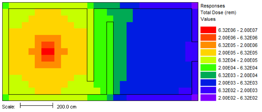
Fig. 4.2.6 Dose (rem) results for the z=100 cm plane (containing the source).
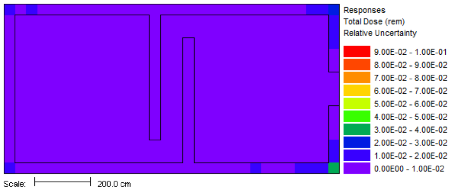
Fig. 4.2.7 Relative uncertainties in the dose, most less than 1%, for the z=100 cm plane.
4.2.5. Summary
SCALE now has the capability to do detailed simulations of criticality accident alarm systems. The advanced variance reduction capabilities of the MAVRIC radiation transport sequence allow for the full three-dimensional analysis of CAAS problems in reasonable amounts of computer time. This enables the use of more realistic source definitions, such as a detailed spatial/energy dependent fission source distribution determined by the KENO-VI criticality code, and the critical assembly itself can be included in the transport model.
References
- CAASMP13a
T.M. Miller and D.E. Peplow. Corrected user guidance to perform three-dimensional criticality accident alarm system modeling with SCALE. In Transactions of the American Nuclear Society, volume 108, 498–501. 1 2013.
- CAASMP13b
Thomas Martin Miller and Douglas E. Peplow. Guidance Detailing Methods to Calculate Criticality Accident Alarm Detector Response and Coverage. Technical Report, Oak Ridge National Laboratory, Oak Ridge, TN (USA), 1 2013. URL: https://www.osti.gov/biblio/1095654 (visited on 2020-08-10).
- CAASMP13c
Thomas Martin Miller and Douglas E. Peplow. Guide to Performing Computational Analysis of Criticality Accident Alarm Systems. Technical Report ORNL/TM-2013/211, Oak Ridge National Laboratory, Oak Ridge, TN (USA), 9 2013. URL: https://www.osti.gov/biblio/1136788 (visited on 2020-08-10), doi:10.2172/1136788.
- CAASPW12
Douglas Peplow and Larry Wetzel. Methods for Detector Placement and Analysis of Criticality Accident Alarm Systems. In Transactions of the American Nuclear Society, volume 106. January 2012.
- CAASPLMP10
Douglas E. Peplow and Jr Lester M. Petrie. Criticality Accident Alarm System Modeling Made Easy with SCALE 6.1. In Transactions of the American Nuclear Society, volume 102, 297–299. 6 2010. URL: http://epubs.ans.org/?a=10467 (visited on 2020-08-10).
- CAASPPJ09
Douglas E. Peplow and Lester M. Petrie Jr. Criticality Accident Alarm System Modeling with SCALE. In Proceedings of the 2009 International Conference on Advances in Mathematics, Computational Methods, and Reactor Physics. 5 2009. URL: http://inis.iaea.org/Search/search.aspx?orig_q=RN:40080894 (visited on 2020-08-10).
- CAASWODonnellN12
L.L. Wetzel, B. O'Donnell, and W.D. Newmyer. CAAS detector placement using MAVRIC. In Transactions of the American Nuclear Society, volume 107, 644–647. 1 2012.