11.5. Data Structures
In the processing of nuclear data, AMPX must accommodate different data structures, all of which are encapsulated in a C++ or Fortran object. This allows easy access to the underlying data independent of the disk format of the data. There are three broad categories of data used in AMPX: (1) point-wise data, which includes cross section data and kinematic data, (2) group-averaged data, which includes all cross section data and matrices in a MG library, and (3) probability data, which includes probability tables and kinematic data in a CE library. In a given category, many of the same manipulations are applicable, and similar coding can be shared for all data structures in the same category.
11.5.1. Point-Wise Data
There are two types of point-wise: (1) 1-D data like cross sections as a function of energy, and (2) kinematic data as a function of incident energy, exit energy, and exit angle. The basic functionalities needed to accommodate point-wise data involve interpolation at any desired energy or angle, basic arithmetic combinations of several point-wise data of the same type, and comparison between two different point-wise data of the same type. AMPX includes template classes that capture parts of the procedure common to all data types and then adds specialization as needed. As in ENDF, a unique number describes each reaction. Reaction numbers are the same as in ENDF, augmented with additional values for special data needed in the transport codes.
Point-wise data allow discontinuities (i.e., there can be two identical energy or angle values with different function values). This frequently occurs if two different evaluations are used in different energy regions. Special care needs to be taken at these points if interpolating or manipulating the data to preserve these discontinuities.
11.5.1.1. 1D Data
1D point-wise data are stored in a format very similar to the TAB1 structure in the ENDF manual [ampx-Her09], which supports energy and cross section values, along with a prescription on how to interpolate the cross section on grid points not given. The same interpolation values as in ENDF are allowed: (1) histogram, in which y is constant in x, (2) linear-linear, in which y is linear in x, (3) linear-log, in which y is linear in ln(x), (4) log-linear, in which ln(y) is linear in x, and (5) log-log, in which ln(y) is linear in ln(x). Internally, AMPX always uses a linear-linear interpolation. Each TAB1 record also includes a header record that contains the reaction number and the temperature of the cross sections data.
11.5.1.2. Kinematic Data
Kinematic data are used in three different forms in AMPX:
\(f\left(E, E^{\prime}, \mu\right)=\frac{d^2 \sigma}{d E^{\prime} d \Omega}\left(E \rightarrow E^{\prime}, \mu\right)\) |
double-differential |
\(f\left(E, E^{\prime}, \mu\right)=\sum_l \frac{2 l+1}{2} a_l\left(E, E^{\prime}\right) P_l(\mu)\) |
Legendre coefficients, and |
\(f\left(E, E^{\prime}, \mu\right)=\sum_l c_l\left(E, E^{\prime}\right)\) |
cosine moments |
where
E is the incident particle energy,
\(E^{\prime}\) exit particle energy,
\(\mu\) is the cosine of the exit angle,
\(P_l(\mu)\) represents the Legendre polynomials of order \(l\),
\(a_l\left(E, E^{\prime}\right)\) represents the Legendre coefficients of order \(l\), and
\(c_l\left(E, E^{\prime}\right)\) represents the cosine coefficients, calculated as \(\int_{-1}^1 f\left(E, E^{\prime}, \mu\right) \mu^l d \mu\)
The kinematic data are stored in C++ classes that allow easy manipulation of the underlying data. The angular distribution for a given incident and exit energy is encapsulated in an ExitEnergy object that stores the exit energy and the angular distribution. An integer flag indicates whether the distribution is given in Legendre moments, cosine moments, or as a tabulated cosine/value distribution. The distribution can be flagged as being discrete, as would be encountered for coherent elastic scattering in crystalline materials. A list of ExitEnergy objects is collected in an IncidentEnergy object, which also stores the value of the incident energy. A flag indicates whether the exit energy distribution describes an elastic or discrete-inelastic reaction, information needed for conversions between center-of-mass and laboratory system. The exit-energy distribution can also be marked as discrete, as would be encountered for discrete gamma lines. A list of IncidentEnergy objects is collected in a KinematicBlock object, which also stores reaction parameters like the reaction type, mass ratios of incident and exit particles, and the Q value. A flag indicates whether the data are given in the center-of-mass or laboratory frame of reference and whether the data are absolute or relative (i.e., divided by the 1D cross section at the given incident energy).
11.5.1.3. Mesh generation
When combining and reconstructing point-wise data, it is often necessary to create an energy or angle mesh for the new distribution. The new mesh is generated by first calculating an initial mesh, most often the union mesh of the distributions to be used in the operation. If any of the distributions has a discontinuity, they are added as a discontinuity to the union mesh. If the distributions do not all start or end at the same energies, the starting and end points are added as discontinuities as well. For example if combining cross section data in the resolved range that ends at Er with cross section from the unresolved range that starts at Er, the energy Er is added twice to the mesh. The mesh is then refined using a halving scheme between two energies or angles: interpolate the distribution at the middle energy or angle and calculate the distribution from an appropriate function and compare the two resulting distributions. If the two distributions agree within a user-supplied precision, the mesh between the two points is dense enough, and the process is repeated with the next set of points. If the two distributions are not the same, the middle energy or angle is added to the mesh, and the process is repeated between the low value and the middle value. A similar procedure is applied to thin the number of mesh points, where the actual distribution at a given energy or angle point is compared to the interpolated distribution. If those two distributions are equal within a user-specified precision, the intermediate energy or angle point is eliminated from the mesh. Mesh points with a discontinuity are never eliminated during a thinning of the mesh. The resulting distribution is calculated on the final mesh. If the new distribution results from an arithmetic operation on other distributions, such as adding or subtracting, special care needs to be taken at discontinuities. If any of the distribution has a discontinuity, it is added as a discontinuity on the final mesh and the calculation is performed twice: once by interpolating the values on the initial distribution on the left side and once on the right side of the discontinuity, which will return the same value if the distribution has no discontinuity. As pointed out, if the contributing distributions do not start and end at the same energy or angle, a discontinuity is added to the final mesh at the starting and ending points and the calculation is performed twice: once with the distribution that starts or ends and once without that distribution.
AMPX has very general codes that combine point-wise data from different distributions of the same type or that generate distributions from a function. The general code calls on specialized functions that interpolate and compare the distribution at a given energy or angle, which are described in more detail below. In addition, the user can supply arithmetic functions that are to be performed on the initial distributions to form the desired distribution or theoretical functions (such as a Maxwellian) to generate a distribution and a suitable mesh.
The advantage of generalized code is that mesh generation and treatment of discontinuities is localized.
11.5.1.4. Interpolation
In the case of 1D data, interpolation at any energy value not given simply uses the interpolation rules (1–5 as described above) to calculate the intermediate value. The same is true if interpolating for a desired angle if the kinematic data are given in double-differential format. All point-wise data can contain discontinuities and interpolation at a discontinuity point can be ambiguous. Therefore, all routines that interpolate point-wise data have a flag indicating whether the left, right, or intermediate value is wanted at the point of the discontinuity. The flag has no effect at other energy or angle values.
11.5.1.4.1. Interpolating in Exit Energy
If the angular distribution is given as Legendre coefficients or as cosine moments, the moments are simply interpolated for the desired exit energy at the correct order using the specified interpolation law. If the angular distribution is given in tabulated form (i.e., as a function of angle cosine), a union mesh of the angles from the two exit energies is formed and refined via a halving scheme. The value for each angle on the resulting mesh is calculated by interpolating the value for the angle at the two exit energies and interpolated at the desired exit energy.
11.5.1.4.2. Interpolation in Incident Energy
For interpolation in incident energy, ENDF and AMPX define additional interpolation laws besides the one defined for other point-wise data: corresponding point interpolation (11–15) and unit-based interpolation (21–25). Assuming there are two distributions—\(f_1\left({E_1,E}^\prime,\mu\right)\) and \(f_2\left({E_2,E}^\prime,\mu\right)\)—where \(f_1\left(E_1, E^{\prime}, \mu\right)\) extends from \(E_1^{\prime l o w}\), to \(E_1^{\prime h i g h}\), and \(f_2\left(E_2, E^{\prime}, \mu\right)\) extends from \(E_2^{\prime l o w}\) to \(E_2^{\prime h i g h}\). The objective is to interpolate \(f_m\left(E_m, E^{\prime}, \mu\right)\). For interpolation schemes 1–5, one proceeds as in the case of angular data, generating an initial union mesh of exit energies as refined by a halving scheme. For each exit energy on the union mesh, the new exit energy distribution is interpolated as described above.
For unit-based and corresponding point interpolation, the lowest exit energy at the intermediate incident energy is
and the highest exit energy is
with a difference in calculating the distributions for intermediate exit energies. In both cases, corresponding exit energies \(\mathrm{E}_1^{\prime}\) in the lower incident energy panel and in the upper incident energy panel are determined. From these, a unit-based value is calculated:
and
which is then interpolated to a value of
and the exit energy in the intermediate panel is
The value of the distribution at \(E_m^{\prime}\) is then calculated using the interpolation law (1–5), obtained by subtracting 10 or 20 from the given interpolation scheme. The difference is in the determination of the corresponding points. If using the unit based approach (21–25), points are chosen so that
For the method of corresponding points (11–15), values \(\mathrm{E}^{\prime} 1\) and \(\mathrm{E}^{\prime} 2\) are chosen so that the normalized cumulative integral over the exit energies agree:
AMPX supports all of the interpolation laws and uses them as given in the evaluation. However, internally, an interpolation value of 22 is used, and additional mesh points are added if needed to describe the distribution as given by the evaluator. The unit-based approach is sensitive to small tails in the distribution since the exit energy range must be well defined. AMPX provides a method that cuts lower or upper exit energies from a distribution if these energies do not substantially contribute to the total integral of the distribution. To determine the new lower exit energy, the integral is calculated first:
and then the partial integral
If \(\left(\frac{\left|I_{tot\ }-I_{part}\right|}{I_{tot}}\right)\) is smaller than a user-defined precision, the energy range is changed to the new lower exit energy. A similar procedure is performed for the upper exit-energy limit.
In addition, the unit-based interpolation is slightly modified if the distribution has upscatter terms in order to preserve the correct upscatter in the interpolated panel. Two units are being used—one extending from \(\left[{E\prime}_{low},E\right]\), and the other from \(\left[{E,\ E\prime}_{high}\right]\), where E is the incident energy. Depending on the distribution and the distance between the provided incident energies, the shape of the exit energy distribution can change, as seen in Fig. 11.5.1.
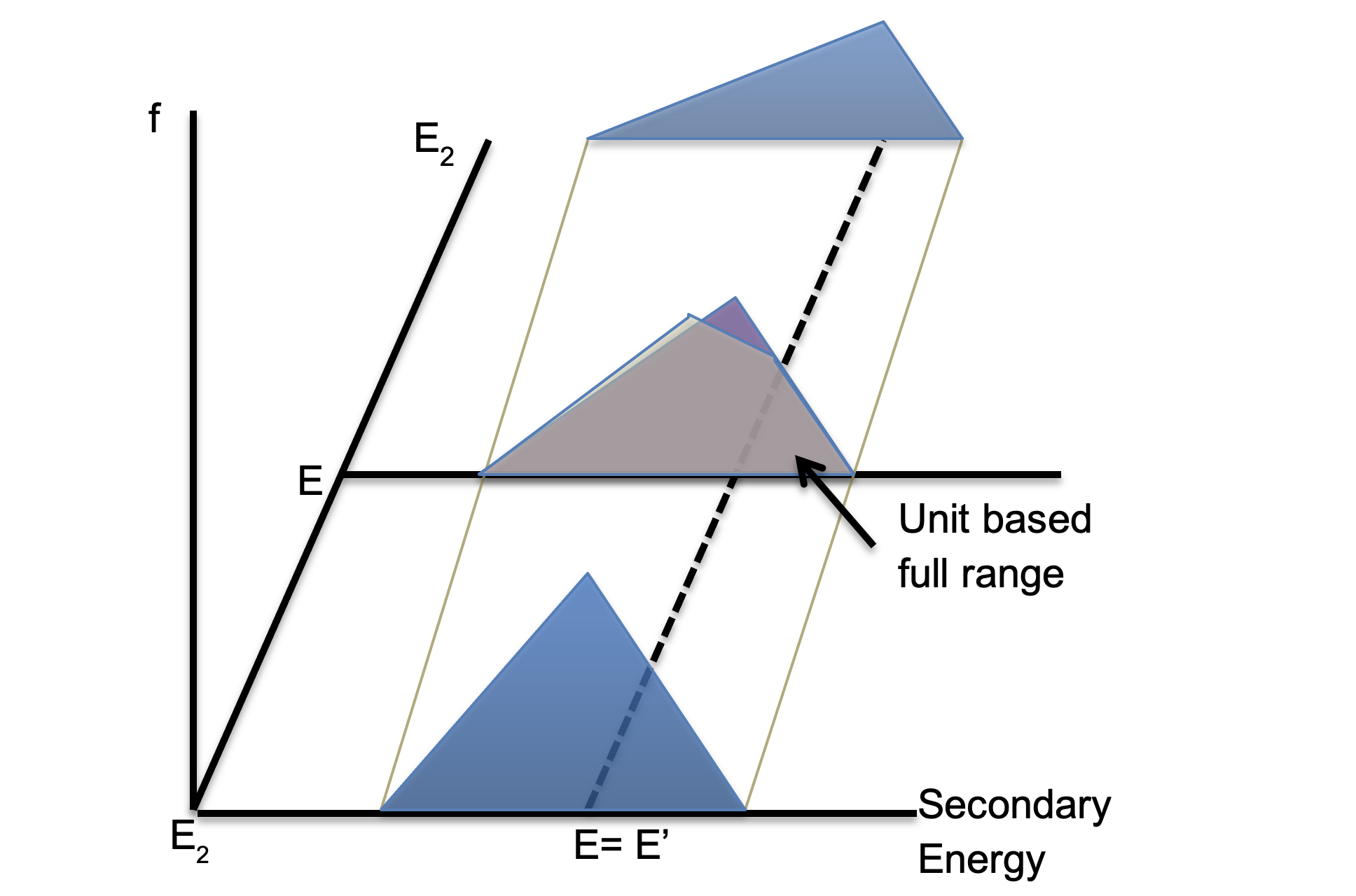
Fig. 11.5.1 Difference between using unit-based over the full range or using unit-based between low exit energy and incident energy and incident energy and high incident energy.
11.5.1.5. Comparison
It is frequently required to compare two values or distributions to determine whether additional data are needed to accurately describe the distribution. Comparison is always made by interpolating a new distribution at the desired energy or angle. While this may be computationally intensive, it provides more precise results. To ensure that two distributions are equal, one steps over a union mesh of energy or angle and interpolates two auxiliary distributions, one from each of the two distributions, to be compared at each union mesh point. These two distributions can now be directly compared. If any of the distributions has a discontinuity, the comparison is made first with the left value then with the right value.
The easiest comparison is for 1D data or angular distributions. As outlined above, values from each point on the union grid are interpolated from both distributions. If any absolute value of those two values is larger than a user-defined cut-off, the two values are assumed to be the same if the relative difference is smaller than a user-defined precision. Otherwise, the absolute difference is compared, which in effect assumes that the two values are zero. The cut-off value ensures that very small values are treated as zero and for example avoids adding unnecessary points to the mesh if comparison is used in connection with a halving scheme. Care needs to be taken so that the cut-off value does not eliminate major features of the distribution. A good choice is a value which, integrated over all energies and/or angles, does not change the total integral more than a user-defined precision. This is the default value chosen in AMPX, but it can be overridden by the user. Two 1D data or angular distributions are equal within in a user-specified precision if all values on the union grid satisfy the above comparison.
Two exit energy distributions are compared by comparing the angular distributions interpolated on the union grid. Two incident energy distributions are compared by comparing the exit energy distributions on a refined union mesh.
Comparison is often used to generate a suitable mesh in incident and exit energy and angle. This procedure works well for exit energy and angles, but it can lead to an extremely fine mesh for the incident energies. Therefore, if an incident energy mesh needs to be refined, then only the exit energy range is compared. If the exit energy range can be interpolated via unit-based interpolation, then the mesh is assumed to be dense enough. In order to thin an incident energy mesh, the full distribution is always used for the comparison. This procedure relies on a good initial grid for the incident energy being given, which is true if the grid is supplied by the evaluator.
11.5.1.6. Conversion for Kinematic Data
Angular distributions for a given exit energy can be given in Legendre or cosine moments or in tabulated form. Conversion functions to convert between these formats are provided in AMPX. Conversion between cosine and Legendre coefficient is a simple transformation of the coefficients: the order does not change. Conversion to tabulated form is always based on Legendre moments. An initial equidistant cosine grid between \(-1\) and 1 is selected on which the Legendre moments are expanded. The grid is refined using the halving scheme described above.
The final kinematic distributions are desired in the laboratory system. Therefore a conversion from the center-of-mass system is often needed. Conversion is only performed for tabulated double-differential formats; a conversion to tabulated format is performed before the conversion if needed.
For elastic and discrete-inelastic incident neutron reactions, there is only one exit energy in the center-of-mass system for a given incident energy, and in the laboratory system, each exit energy has exactly one exit angle. To convert the kinematic data for a given incident energy, AMPX generates an initial grid of exit energies in the laboratory system by stepping over equidistant points in the angle distribution in the center-of-mass system. The grid is then further refined by a halving scheme used on the center-of-mass angle until the exit and angle distribution in the laboratory system can be reproduced to a user-defined precision. For some nuclides and reactions, two different exit energies in the laboratory system can have the same exit angle. In these cases, the Jacobian that transforms the value of the distribution from center-of-mass to laboratory system can be infinite, and the above halving system does not work correctly when close to the discontinuity. In these cases, the angle in the center-of-mass system where the discontinuity occurs is determined, and two laboratory angles on either side of the value are chosen so that the Jacobian can still be calculated within numerical precision. The halving scheme is then employed on the center-of-mass angles below the lower of the two angles and above the higher of the two angles. In addition, a much denser initial grid is chosen for the lower angular region. If the final format is moments instead of tabulated, the Jacobian for the transformation from center-of-mass to laboratory system is not required for the angle, as integration is performed over the whole angle range. Therefore, the Jacobian to convert between center-of-mass and laboratory system angle is not applied, and the distribution is immediately converted to cosine moments. The Jacobian to convert between center-of-mass and laboratory system exit energies is still applied. If the distribution is desired in tabulated form, both Jacobians are applied.
The incident energy grid used in the center-of-mass system can often be coarser than is required in the laboratory system, especially for threshold reactions. Additional incident energies in the laboratory system are calculated by interpolating a distribution for the desired incident energy from the center-of-mass kinematic data and then converting the distribution to the laboratory system as described above. The additional incident energies are chosen so that the exit energy range can be determined via unit-based interpolation. The exit energy distributions themselves are not compared. The laboratory incident energy grid is thinned if possible, but this time it is based on a full comparison of the exit energy and angle distribution.
The procedure to convert other reactions from center-of-lab to the laboratory system is similar to the conversion for elastic incident neutron reactions except that there can be more than one exit angle for a given exit energy. In this case, the distribution in the center-of-mass and laboratory system will always be tabulated; there is no special treatment if the final desired format is an angular distribution in moments.
If the kinematic data for a threshold reaction are given in the center-of-mass system, ENDF sometimes contains exit energy distributions at incident energy slightly below or at the threshold. Conversion of these panels to the laboratory system is numerically unstable. Therefore, only incident energies slightly above the threshold are converted. In order to preserve the distribution, additional incident energies above the threshold are inserted into the distribution in the center-of-mass system before conversion to the lab system.
11.5.2. Group-Averaged Data
Group-averaged data used by AMPX are categorized in three broad groups: (1) 1D cross section data, which includes f-factors and subgroup data, (2) scattering matrices and (3) group-averaged covariance data. 1D cross section data and scattering matrices are normally contained in a MG library. AMPX and SCALE share a C++ resource that keeps all MG data in memory and provides classes to access the data.
An integral over one set of 1D data can always be calculated analytically since the interpolation is known. AMPX library functions provide methods for this simple integral.
The two point-wise data structures described above can be converted to group-averaged data using AMPX library functions. In the case of 1D cross section data, a point-wise cross section TAB1 object is multiplied with a flux, which is also given as a TAB1 object, and then it is integrated over all energies in a given group:
where \(\sigma\left(E\right)\) is the cross section and \(\varphi\left(E\right)\) is the flux. The yield \(y\left(E\right)\) is only different from 1 if fission yields are calculated. This integral can be solved numerically if the two distributions use linear interpolation.
Scattering matrices are calculated for a given incident energy group and exit energy group, and they are always in Legendre moments. Please note that AMPX includes a \((2l+1)\) factor for each matrix, where l is the order of the Legendre moment. Assuming the incident energy group i has boundaries \(\left\lfloor E_1,E_2\right\rfloor\) and the exit energy group j has boundaries \(\left\lfloor{E^{\prime}}_1,{E^{\prime}}_2\right\rfloor\), the scattering matrix element at \([i,j]\) for Legendre moment l is calculated as:
where \(\sigma\left(E\right)\) is the cross section, \(\varphi\left(E\right)\) is the flux, and \(f_l\left(E,E^{\prime}\right)\) is the exit energy distribution at incident energy E for the lth Legendre order . The yield \(y\left(E\right)\) is only different from 1 if fission yield matrices are calculated. The inner integral at a given energy E is calculated using unit-based interpolation. Assuming the desired incident energy \(E_m\) lies between two incident energies present in the distribution—\(f_l\left(E_1, E^{\prime}\right)\) and \(f_l\left(E_2, E^{\prime}\right)\)—the exit energy range \(\left[E_m^l, E_m^h\right]\) is calculated at \(E_m\) using Eq. (11.5.1) and Eq. (11.5.2), from which the unit-based exit group boundaries \(x_1^{\prime}=\frac{E_1^{\prime}-E_m^l}{E_m^h-E_m^l}\) and \(x_2^{\prime}=\frac{E_2^{\prime}-E_m^l}{E_m^h-E_m^l}\) are calculated in the intermediate panel. From this the corresponding x values can be calculated, as well as the integral boundaries in the two outer distributions. The integrals for the two outer distributions are then calculated, and a value at \(E_m\) is calculated by linear interpolation of the integrals. The outer integral is performed for all cosine orders at the same time using a fourth order Runge–Kutta method with adaptive step size [ampx-PVTF92], except when the angular distribution is discrete and the integral can be calculated analytically.
11.5.3. Probability Data
For CE libraries, the kinematic data are needed in marginal (with respect to angle) and conditional (with respect to exit energy) cumulative probability functions. In the case of elastic and discrete inelastic reactions, the conversion is straightforward, as there is only one possible exit energy for a given exit angle. Thus the marginal cumulative probability function is simply the normalized angular distribution. For each angle, the conditional cumulative probability function has one value.
For other reactions, the code first determines an angular mesh for each incident energy that is dense enough so that the angular distribution for each exit energy can be represented on that mesh. On that incident energy-dependent angle mesh, \(f\left(E, E^{\prime}, \mu\right)\) is integrated over all \(E^{\prime}\) values. The integral of this function in angle is the yield. This function, normalized so that the integral is 1, is the cumulative distribution in angle for the given incident energy. The cumulative distribution function is divided into a user-defined number of equiprobable bins, usually 32. If the distribution function can be described with less than the user-defined number of bins that are not equiprobable, then that grid is used instead to conserve disk space. For each bin, the conditional cumulative probability distribution for the exit energies is determined and saved.