2.2. CSAS-Shift: Criticality Safety Analysis Sequence with Shift

K. B. Bekar, G. Davidson, B. Langley, B.J. Marshall

The CSAS-Shift sequence integrates the Shift advanced Monte Carlo solver into the CSAS framework as an alternative to the KENO transport solvers to perform reliable and efficient eigenvalue calculations for criticality safety and reactor physics analysis. It supports both KENO V.a and KENO-VI geometries and provides most widely used KENO capabilities available in the CSAS5 and CSAS6 sequences for both multigroup and continuous-energy transport modes. The highly scalable Shift Monte Carlo solver enables faster solutions when running on multiple cores, and it shows better performance to achieve the same level of accuracy compared to the CSAS sequences with the KENO codes.

2.2.1. Introduction

The CSAS-Shift sequence was designed to provide the modeling and simulation capabilities required for criticality safety and reactor physics analysis through the Shift Monte Carlo solver.

Shift is a massively parallel Monte Carlo radiation transport package in the Exnihilo radiation transport code suite [CSAS-ShiftPJE+16], [CSAS-ShiftESSC10]. Shift was developed including features such as support for both fixed-source and eigenvalue Monte Carlo transport capabilities with multiple geometry and physics engines, hybrid capabilities for variance reduction methods, and advanced parallel decompositions to scale well from laptops to small computing clusters to advanced supercomputers. Shift supports different geometry engines, including the Oak Ridge Adaptable Nested Geometry Engine (ORANGE) designed to provide particle transport capabilities on both KENO V.a and KENO-VI geometries as well as geometry visualization capabilities in the Fulcrum user interface. Shift with both versions of KENO geometries performs eigenvalue calculations in both continuous-energy and multigroup modes. Shift supports most widely used primary capabilities available with the KENO codes and provides some unique capabilities with ORANGE such as modeling randomly packed media and efficient parallel calculations for volume estimates.

CSAS-Shift provides all capabilities for both multigroup and continuous-energy transport modes. Like the CSAS5 and CSAS6 implementation, in the multigroup calculation mode, CSAS-Shift sequences automate the processing of the cross sections for temperature corrections and problem-dependent resonance self-shielding for utilization in multigroup neutron transport calculations using SCALE’s cross section processing module, XSProc. If continuous-energy calculation mode is selected, no resonance processing is needed, and the continuous-energy cross sections are used directly in the Shift code, with temperature corrections provided as the cross sections are loaded.

CSAS-Shift with the highly scalable Shift solver enables some unique capabilities and faster solutions when running on multiple cores, and it shows better performance to achieve the same level of accuracy compared to the CSAS sequences with the KENO codes. CSAS-Shift input requirements, supported and unsupported capabilities, and input and output details are described in the following sections.

2.2.2. CSAS-Shift Input Requirements

CSAS-Shift’s design is aimed to make a smooth transition between KENO codes to the Shift transport code. Therefore, the original input data layout available in CSAS sequence with the KENO transport codes was kept the same for the CSAS sequence with Shift transport. CSAS-Shift uses the same CSAS5 and CSAS6 inputs, the only input modification that should be required is changing the sequence name by appending -shift to the sequence name, as shown in Example 2.2.1.

Like CSAS sequences with KENO codes, CSAS-Shift sequences are named with the KENO geometry that they support: CSAS5-Shift for the models with KENO V.a geometry, and CSAS6-Shift for the models with KENO-VI geometry.

Example 2.2.1 CSAS sequence inputs with KENO and Shift transport

=csas5
Godiva sphere
ce_v7.1

read composition
   u-234       1 0 0.000491995 300   end
   u-235       1 0 0.0449996 300   end
   u-238       1 0 0.002498 300   end
end composition

read parameter
   html=no
end parameter

read geometry
   sphere 1 1   8.741
end geometry

end data
end

=csas5-shift
Godiva sphere
ce_v7.1

read composition
   u-234       1 0 0.000491995 300   end
   u-235       1 0 0.0449996 300   end
   u-238       1 0 0.002498 300   end
end composition

read parameter
   html=no
end parameter

read geometry
   sphere 1 1   8.741
end geometry

end data
end

Warning

CSAS-Shift sequence implementation may ask the user for some minor input updates for a successful calculation.

2.2.3. Sequence Capabilities

In the CSAS-Shift sequence framework, SCALE data handling is automated as much as possible. Similar to many other SCALE sequences, CSAS-Shift also applies a standardized procedure to provide appropriate number densities and cross sections for the calculation. XSProc is responsible for reading the standard composition data and other engineering-type specifications—including volume fraction or percent theoretical density, temperature, and isotopic distribution, as well as the unit cell data. XSProc then generates number densities and related information, prepares geometry data for resonance self-shielding and flux-weighting cell calculations, and (if needed) provides problem-dependent multigroup cross section processing.

Sequences that execute Shift transport include a data processor named ExnihiloInputBuilder to read and check the KENO data. This data processor processes the KENO data and creates a ParameterList input used by Shift to construct the problem and perform transport calculations. When the data checking has been completed, the CSAS-Shift sequence executes XSProc to prepare a resonance-corrected macroscopic cross section library in the AMPX working library format for the subsequent Shift transport calculation if a multigroup library has been selected.

Similar to CSAS sequences with KENO transport, the CSAS-Shift sequence supports both CELLMIX and Double-het capabilities. For each unit cell specified as being cell-weighted, XSProc performs the necessary calculations and produces a cell-weighted macroscopic cross-section library. Shift may be executed to calculate the k-effective, or neutron multiplication factor, using the cross section library that was prepared by the control sequence.

Computational capabilities available in CSAS sequences with KENO codes—including the determination of k-effective, flux densities, fission densities, mesh tallies, Shannon entropy tally, problem-dependent continuous-energy temperature treatments, parallel calculations, and many more—are also provided by the CSAS-Shift sequence.

CSAS-Shift also supports two new CSAS sequence data blocks, definitions and tallies data, to allow flexible definition and output control of mesh tallies. The mesh responses neutron flux, fission rate, and fission source can now be requested multiple times on different spatial and energy grids in the same calculation. This capability helps users efficiently manage computational resources when collecting detailed information, depending on their requirements.

Criticality safety tools in SCALE attain some unique capabilities provided by Shift with the new geometry engine ORANGE, such as parallel volume estimates for KENO-VI geometric regions and modeling randomly packed media, which is enabled by implementing a random-packing algorithm to place spherical particles within simple bounding geometries. This capability allows constructing tristructural isotropic (TRISO) particle models for advanced reactor modeling and simulation activities. See Sect. 2.2.4.1.2.1 for further details.

Details for some of these capabilities, their input methods, and output edits are provided in the following sections.

2.2.3.1. Multigroup limitations

Some of the limitations of the CSAS-Shift multigroup sequences are a result of using preprocessed multigroup cross sections. Inherent limitations in multigroup CSAS-Shift calculations are as follows:

1. Spatial effects such as fuel rods in assemblies where some positions are filled with control rod guide tubes, burnable poison rods, and/or fuel rods of different enrichments. The cross sections are processed as if the rods are in an infinite lattice of identical rods. If the user inputs a Dancoff factor for the cell (such as one computed by MCDancoff), XSProc can produce an infinite lattice cell which reproduces that Dancoff. This can mitigate some spatial lattice effects.

2.2.3.2. Continuous-energy limitations

The continuous-energy cross sections are directly used in Shift. An existing multigroup input file can easily be converted to a continuous-energy input file by simply specifying the continuous-energy library. In this case, all cell data is ignored. However, the following limitations exist:

1. If CELLMIX is defined in the cell data, the problem will not run in continuous-energy mode. CELLMIX implies new mixture cross sections are generated using XSDRNPM-calculated cell fluxes; therefore it is not applicable in continuous-energy mode.

2. Problems with DOUBLEHET cell data are not allowed, as they inherently utilize the CELLMIX feature.

2.2.3.3. Unsupported Capabilities

Although Shift Monte Carlo code was designed with several advanced capabilities, it does not currently support some of the unique features available in KENO codes. Therefore, CSAS-Shift does not provide some of the capabilities available in CSAS5 and CSAS6 sequences.

The missing capabilities are mostly considered as the outdated features or those seldomly used by CSAS users in their analysis. The equivalent capabilities will be activated in the Shift transport code in the next SCALE release, depending on the need basis.

Table 2.2.1 summarizes the capabilities currently supported by CSAS with KENO codes but not supported by CSAS-Shift sequences.

Table 2.2.1 Unsupported CSAS capabilities

Capability	Input method(s) to activate the capability	Comments
Adjoint transport	parameter data ADJ	Adjoint transport capability is not available in Shift
Prompt-only \(nu\)	parameter PNU	Shift does not support using prompt neutron spectrum only in continuous-energy mode
Use unionized mixture cross section	parameter UUM	Shift does not support KENO-like mechanism to store cross sections on a material-based unionized energy grid for a faster cross section lookup in continuous-energy mode Although this method benefits for faster runtimes for some KENO models, storing all data may require prohibitively large amount of memory for problem with a large number of materials. Different approaches are being developed in Shift transport, and some experimental implementation is available in CSAS-Shift. See Table 2.2.4 for more details.
Matrix k-effective	parameters MKP, CKP, FMP MKU, CKU, FMU MKH, CKH, FMH MKA, CKA, FMA HAL, HHL, FMA	An alternative k-effective calculation method available in KENO codes are not supported by Shift.
Start data types 2, 3, 4, 5 and 9	start data block NST= 2, 3, 4, 5, and 9	Start data types 2 - 5 have not been implemented by ORANGE geometry engine used by Shift transport. Start type 9 designed to read starting distribution from a mesh source file is not currently supported by CSAS-Shift.
Biasing or weighting data	bias data block	KENO-like biasing capability is not currently supported by Shift transport.
Periodic and White Albedo boundary conditions	bounds data block	Shift transport does not currently support PERIODIC and WHITE boundary conditions for both KENO V.a and KENO-VI geometries.
Differential Albedos	bounds data block, PAX in parameter data block	Material specific albedos available with KENO multigroup transport is not supported by Shift multigroup transport
LOOP construct in array data	array data block	LOOP construct in array data input block is not supported by ORANGE geometry engine as part of Shift code.
Volume calculation (random sampling)	type=RANDOM in volume data block	Random volume estimates for KENO-VI geometry is not available in ORANGE geometry engine used by Shift transport
Accumulate mesh fluxes	parameter MFX	Shift does not support to tally mesh fluxes which are averaged over the region volumes in each mesh voxel.
Compute and print mean free paths	parameter MFP	This capability is not currently implemented in Shift.
Region-dependent fissions and absorptions	parameters FAR and GAS	Although these tallies are available in Shift transport they are not currently implemented in CSAS-Shift.
Mixture-dependent reaction tallies	reaction data block	Although these tallies are available in Shift transport they are not currently implemented in CSAS-Shift.
Time controlled termination	parameter TME	Shift does not have job termination capability controlled by the user-defined time limit.
Terminate execution on user signal	by creating a file named stop_keno in the working directory	CSAS-Shift does not support this capability
Restart capability	parameters RES, BEG, APP, RST, WRS	Restart capability is not available in Shift
Print particle tracks	parameter TRK	Although Shift has its own mechanisms to print information about each particle history, this capability is not fully integrated in CSAS-Shift sequence. It will be available in next releases.
Problem Characterization Output Edit	always ON	CSAS-Shift implements the nu bar, average fission group energy of the average lethargy causing fission and system mean free path in this output edit. Lifetime and generation time are not currently available.
Plots of avg. k-effective and Shannon entropy	always ON	CSAS-Shift does not produce char-plots for the average k-effective by generations run, the k-effective by generations skipped, and Shannon entropy per generation. Instead of the char-plots, CSAS-Shift creates Ptolemy plots and stores them in a dedicated plot directory. Fulcrum may be used to visualize these plots. See Sect. 2.2.6.1.13
Summary of Source Convergence Diagnostics	parameter SCD	CSAS-Shift does not perform the posterior entropy tests available in KENO. Instead, result of a single test performed by Shift is captured and printed in the relevant output section.
Print capabilities for mixed cross section	parameters AMX, XS1, XS2, PKI P1D, XAP, XSL	Currently, no capability is available to print the cross sections used by Shift transport.
Flux moments and angular flux calc.	parameters TFM, PMF, PMM	CSAS-Shift does not support any of these capabilities.
Print starting points	PSP parameter in start data	This capability is not currently implemented in CSAS-Shift
Plot capability	parameter PLT plot data block	Old-style plotting capabilities available in KENO codes are not supported. Fulcrum can be used for geometry visualization.
HTML output	parameter HTM	Old-style HTML-based output method is not supported.

2.2.4. Input Data Guide

This section describes the input data required for the CSAS-Shift sequence. A typical CSAS6-Shift input, shown in Example 2.2.2, starts with the sequence identifier always preceded by the = sign, and it is followed by the problem title. Then, a cross section library name is specified, and all these entries are followed by several data blocks each starting with READ data_block and ending with END data_block.

Example 2.2.2 A typical CSAS-Shift sequence input

  =CSAS6-Shift parm=(parm_options)
  problem title

  ' ----- XSProc data
  ' cross section library name (REQUIRED)
  ce_v7.1

  ' List of material specifications in standard SCALE format (REQUIRED)
  read composition
     ...
  end composition

  ' Specify data for resonance processing (OPTIONAL)
  read celldata
     ...
  end celldata

  ' ---- New CSAS sequence data blocks

  ' Used to define energy bounds and grid geometries for
  ' the tallies defined in tallies data block
  ' (REQUIRED if tallies data block exists)
  read definitions
     ...
  end definitions

  ' Used to define tallies in a more robust way (OPTIONAL)
  read tallies
     ...
  end tallies

  ' ---- KENO transport data
  ' Specify the problem geometry (REQUIRED)
  read geometry
     ...
  end geometry

  ' Other input data blocks (OPTIONAL)

Because CSAS-Shift uses the same input data used by CSAS5 and CSAS6, details of the input data blocks, compositions, celldata, definitions, and tallies will not be repeated here, and they can be seen in Sect. 2.1.4. Data blocks in the KENO transport data category will be discussed in the following section.

Note

For CSAS-Shift, the grid boundaries must be inside the specified geometry, while CSAS-KENO permits grid boundaries beyond the geometry.

2.2.4.1. KENO input data in CSAS-Shift

Table 2.2.2 presents the lists of the KENO input data blocks supported by CSAS-Shift sequence. The input method in some data blocks may show some minor differences between the CSAS-KENO and CSAS-Shift sequences. Similarly, some capabilities provided by each input block also have some differences. All these details are discussed in this section. KENO input data blocks, that are reaction data, bias data, mixt data, and plot data, are not currently supported by the CSAS-Shift sequences.

Table 2.2.2 Summary of KENO input data blocks available in CSAS-Shift sequences.

Data block	Status	Comments
Parameters*	Supported	See Sect. 2.2.4.1.1 for more details.
Geometry	Supported	See Sect. 2.2.4.1.2 for more details.
Array data	Supported
Boundary conditions	Supported	See Sect. 2.2.4.1.2 for more details.
Volume data	Supported	See Sect. 2.2.4.1.2 for more details.
Energy boundaries	Supported
Start data	Supported	See Sect. 2.2.4.1.3 for more details.
Grid geometry data	Supported
Plot data	Not available	The data in this block will be ignored in the calculations
Bias data	Not available	Execution will be terminated.
Reaction data	Not available	The data in this block will be ignored in the calculations
Mixt data	Not available	The data in this block will be ignored in the calculations
* Must precede all other data blocks in this table.

Similar to CSAS5 and CSAS6, geometry data is the only KENO data block required to perform Shift transport calculation as part of the CSAS-Shift sequence. Other data blocks are optional, and the same default values listed in various locations in Sect. 8.1 are also applied to the data in each data block in CSAS-Shift. Note that parameter data must precede all other KENO data blocks if it is entered.

When CSAS-Shift is run with a user input including bias data block, the execution will be terminated with the error message given in Example 2.2.3. Note that CSAS-Shift ignores the data entered in the unsupported plot data, mixt data, and reaction data blocks and continues the calculation. User is notified with a warning message as shown in Example 2.2.4.

Example 2.2.3 Error message printed by CSAS-Shift output when biasing data is found in user input.

      ***Error: Failed to run ExnihiloModule with assertion:
      ----------------------------------------------
       These input cards are unsupported by Shift.
      ----------------------------------------------
       They must be removed from the input to run.
      ----------------------------------------------
       line: 19   column: 1   biasing
      ----------------------------------------------


       ^^^ at /ornldev/code/Scale/S63/Source/packages/Module/Exnihilo/InputProcessorBase.cpp:193

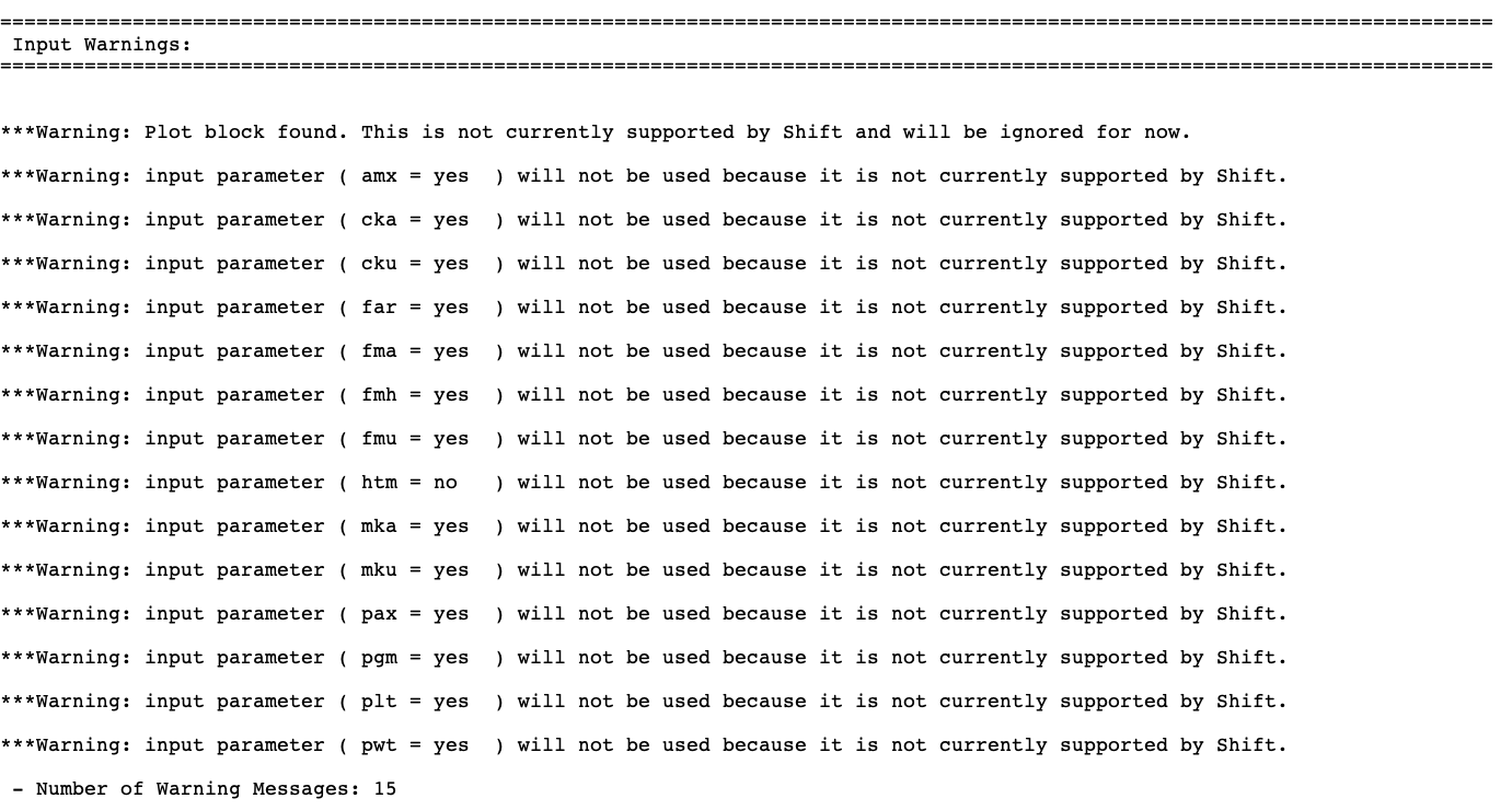
Example 2.2.4 A typical warning message printed by CSAS-Shift output when an unsupported data block is found in user input.

  ====================================================================================================
  Input Warnings:
  ====================================================================================================

  ***Warning: Plot block found. This is not currently supported by Shift and will be ignored for now.

Note

CSAS5-Shift and CSAS6-Shift also support PARM=CHECK or PARM=CHK sequence parm options. This will allow checking the input data without performing cross section calculation as well as Shift transport calculations.

=CSAS6-SHIFT PARM=CHK

2.2.4.1.1. Parameter data

The KENO parameter data block in both CSAS5 and CSAS6 sequences provides many control parameters to activate the capabilities available in KENO transport for the problem being run. CSAS-Shift supports only a subset of these parameters, as listed in Table 2.2.3. Detailed description of these parameter can be seen in Sect. 8.1.3.3.

Parameters entered in the parameter data input block are processed by CSAS-Shift sequence implementation, and then the ParameterList input is updated to accordingly activate/deactivate the equivalent capabilities with Shift transport if the asking feature is currently supported by Shift. CSAS-Shift usually ignores the unsupported parameters by notifying the user with a warning message, and then it continues the calculation. For some specific parameters, code can terminate the execution and ask the user to remove this parameter from the input and rerun the code for a successful calculation.

Caution

CSAS-Shift notifies users of the unsupported parameters with a warning message before Numeric and Logical Parameters edit in the output, and then it ignores this parameter. It is the user’s responsibility to examine which input parameter is ignored in the current calculation.

Note

CSAS-Shift defaults the value of a parameter, which is currently supported but not defined in the parameter data input block, to the KENO default. In other words, both CSAS and CSAS-Shift use the same defaults for the same parameters.

Table 2.2.3 Summary of KENO parameters currently supported by CSAS-Shift

PARAMETERS:		Format: READ PARAM parameter_data END PARAM See Sect. 8.1.3.3 for details.
KEY	DEFAULT	DEFINITION	KEY	DEFAULT	DEFINITION
RND=	given	random number	THC=	10.0	thermal energy cutoff (eV)
SIG=	0.0	deviation limit	DBL=	0.4	DBRC lower energy cutoff (eV)
WTA=	0.5	average weight	DBH=	210	DBRC upper energy cutoff (eV)
WTL=	1/WTH	Russian Roulette weight	MSH=	0.0	mesh size of the cubic mesh
GEN=	203	number of generations	DBR=	0	use DBRC for scattering
NPG=	1000	number per generation	DBX=	2	Doppler Broadening method
NSK=	3	generations skipped	CET=	0	CE TSUNAMI calculation mode
NGP=	252	number of energy groups for tallying	CFP=	-1	number of latent generations for CE- SUNAMI
PTB=	YES	use probability tables	SCD=	YES	fission source convergence diag.
FLX=	NO	collect and print region fluxes	CDS=	NO	accumulate neutron production
FDN=	YES	fission densities	FIS=	NO	fission rate mesh tally
NUB=	YES	neutrons per fission	GFX=	NO	compute grid fluxes
FST=	NO	print F*(r) 3dmap	CGD=	NO	use mesh for CLUTCH F*(r) calc.
RUN=	YES	execute problem	TRK=	NO	NOT FULLY IMPLEMENTED

Table 2.2.4 Summary of parameters available only in CSAS-Shift

PARAMETERS:
KEY	DEFAULT	DEFINITION
PN_ORDER=	5	Legendre polynomial order
DOUBLE_INDEXING=	0.0	Accelerate xsec calculation using double indexing
THINNING_TOLERANCE=	0.0001	Tolerance to use thinning the unionized xsec grid

In CSAS5 and CSAS6, users can control the number of scattering angles in multigroup calculations by entering the SCT parameter in the KENO mixing data block. The similar capability in CSAS-Shift was provided by adding a new parameter, PN_ORDER=, to the parameter data block because the mixing data block is not supported by CSAS-Shift sequences. Its default is set as 5.

2.2.4.1.2. Geometry data

CSAS-Shift with ORANGE geometry supports all KENO V.a and KENO-VI geometry capabilities except the following:

• LOOP construct in array data block

• Material-specific albedo boundary conditions

• PERIODIC and WHITE albedo boundary conditions

• Random volume estimates for KENO-VI geometry (TYPE=random option in volume data)

CSAS-Shift can perform volume calculations with the stochastic ray-tracing method concurrently on the replicated domain on multiple cores.

2.2.4.1.2.1. Random geometry

Another new capability in CSAS-Shift is the automatic placement of units within another unit. This capability is currently limited to the stochastic placement of spherical geometries without clipping within another geometry. Additional options such as the automatic placement in lattice structures and the extension to other geometries is planned for future SCALE releases.

This new capability is enabled through a new input block named randomgeom. The randomgeom block is composed of randommix specifications which is again composed of key/value pairs. The basic structure of the randomgeom block and the randommix specifications is as follows:

Example 2.2.5 New randomgeom data block in CSAS-Shift

 read randomgeom

     RANDOMMIX = ID
        TYPE=random
        UNITS= U1 U2 ... UN end
        PFS= pf1 pf2 ... pfN end
        CLIP= no
        SEED= int
     end RANDOMMIX

 end randomgeom

with

• RANDOMMIX - keyword with ID number or name

• TYPE - distribution type of units (currently limited to random)

• UNITS - list of unit number(s) to be distributed in geometry

• PFS - fraction of volume occupied by units U1 ... UN

• CLIP - boundary clipping (currently limited to no)

• SEED - random seed for random placement

Similar to the array block, this input block requires that the unit specified as part of a randommix in the units list must exist in the geometry. An additional requirement is that the the units must have a spherical outer boundary. The PF list must have the same length as the units list. The sum of the values listed in PFS must be less than 1.0. In practice, the actual limit to the total PF depends on the size and number of the units specified by the user. The TYPE keyword specifies the distribution of the units within the geometry. The type is currently limited to random which will call a stochastic placement algorithm to randomly distribute the units in the geometry. The CLIP keyword controls the clipping of the units along the geometry in which they are placed. This is currently limited to no, that is the units are not clipped by the geometry. The SEED keyword is specifying the random seed used for the stochastic distribution of units. This assures the same random distribution if the input is run multiple times.

Note

Given the stochastic algorithm that is currently called by the randommix block, in practice total packing fractions of up to approximately 20% are achieved.

A “fill” material—the interstitial media surrounding the random spherical geometry units—is not present in the randomgeom block. Instead, the fill media is handled in the unit specification within the KENO geometry block of the input file: A region in a unit is filled with both a media and a randommix record. Then the media is filling the space of the region that is not occupied by units placed through the units defined in the randommix record. A randommix block can be used in multiple different units with varying fill materials. The basic unit format along with a randommix on the media record itself is as follows:

Note

A randommix can currently be filled only into regions that have an outer boundary of a sphere, cuboid, or cylinder.

read randomgeom
   randommix=ID
      ...
   end randommix
end randomgeom

read geometry
   ...

   unit U
      surfaces ...
      media ...
      media F biasID surfaces randommix=ID
      boundary S
   ...

end geometry

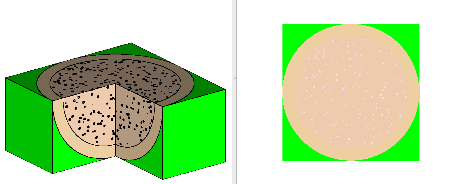
In the sample case shown in Example 2.2.6, a single pebble is filled with a single TRISO particle type. Fig. 2.2.1 shows how TRISO particles are placed in a single pebble with the randomgeom capability. The individual location of particles is written in the Shift Hierarchical Data Format (HDF5) output file, so these locations can be used for verification or other purposes as needed.

Example 2.2.6 One TRISO type in a pebble

=csas6-shift
...

read geometry
   unit 1
      com='kernel1'
      sphere 1 2.50e-02
      sphere 2 3.40e-02
      sphere 3 3.80e-02
      sphere 4 4.15e-02
      sphere 5 4.55e-02
      media 100 1 1
      media 101 1 2 -1
      media 102 1 3 -2
      media 103 1 4 -3
      media 104 1 5 -4
      boundary 5
   global unit 10
      com='pebble'
      sphere 1 2.5
      sphere 2 3.0
      cuboid 3 6p5.0
      media 101 1 1 RANDOMMIX='trisos'
      media 106 1 2 -1
      media 0 1 3 -2
      boundary 3
end geometry
read randomgeom
   randommix = 'trisos'
      type= random
      units= 1 end
      pfs= 0.05 end
      clip= no
      seed= 0
    end randommix
end randomgeom

end data
end

Fig. 2.2.1 Visualization of 3D and 2D cuts of the single TRISO model.

2.2.4.1.3. Start data

CSAS-Shift supports only START types 0, 1, 6, 7, and 8. CSAS-Shift start data implementation does not currently support the PSP option, which is used to print source positions sampled by the Shift transport.

Implementations for start types 0, 1, 7, and 8 in CSAS-Shift are are similar to those in CSAS5 and CSAS6. However, there are some minor differences in start type 6.

In KENO start type 6 implementation, the following rules are applied when selecting the starting points (see Sect. 8.1.4.8 and Sect. 8.1.3.3 for more details).

• Start NPG initial fission neutrons at first-NPG starting points defined by start type 6 data if NPG < LNU. Remaining starting points beyond NPG will be discarded.

• Start NPG initial fission neutrons at LNU starting points defined by start type 6 data if NPG = LNU.

• Start LNU initial fission neutrons at the starting points defined by start type 6 data, then randomly select the remaining fission source points (NPG-LNU) from these starting points if NPG > LNU.

where LNU, a start type 6 data parameter, is the total number of starting points specified in the start data block; and NPG, a parameter in the parameter data block, is the number of neutrons per generations.

Unlike KENO, the CSAS-Shift input processor does not follow the above rules when selecting positions for the initial fission neutrons. It calculates the probability of each point being selected and passes all starting points with this information to the Shift module. The Shift module always samples NPG initial fission source points using these data.

For example, the KENO code processes the following input and then samples the initial fission points.

=csas6 parm=bonami
Godiva test problem
test-8grp

read composition
   u-234       1 0 0.000491995 300   end
   u-235       1 0 0.0449996 300   end
   u-238       1 0 0.002498 300   end
end composition
read parameter
   htm=no gen=10 npg=15
end parameter

read geometry
   global unit 1
      sphere 1 8.67
      media 1 1 1
      boundary 1
end geometry

read start
   nst=6 ps6=yes psp=yes
   tfx=1.0 tfy=1.0 tfz=1.0 lnu=5
   tfx=2.0 tfy=2.0 tfz=2.0 lnu=20
end start
end data
end

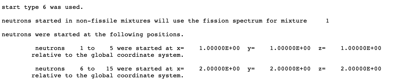
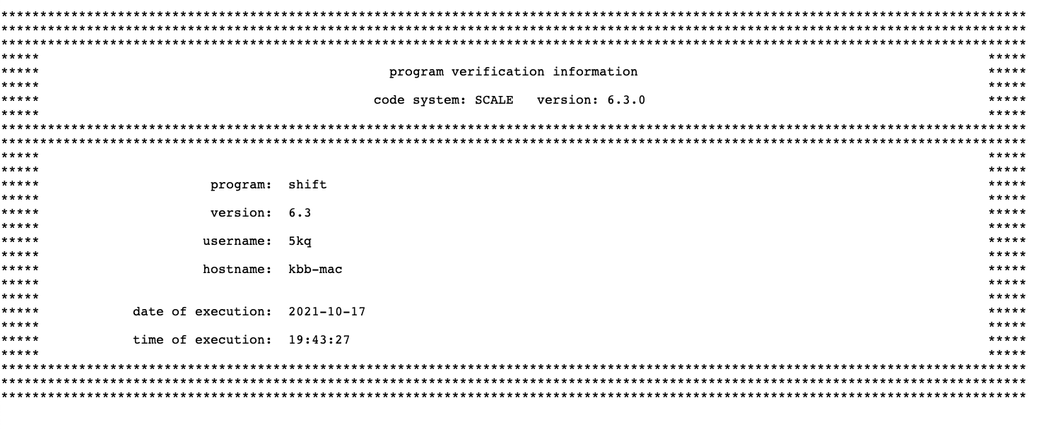
The summary of the sampling process is printed in KENO output, as shown in Fig. 2.2.2. KENO first starts 5 neutrons at (1.0, 1.0, 1.0) and the remaining 10 neutrons at (2.0, 2.0, 2.0) since LNU=20 > NPG=15.

Fig. 2.2.2 Start type 6 output printed by CSAS6.

However, CSAS-Shift creates a probability distribution from the defined start type 6 points and samples starting positions for NPG=15 particles using this distribution, as shown in Fig. 2.2.3.

Fig. 2.2.3 Start type 6 output printed by CSAS-Shift.

2.2.5. Notes to CSAS-Shift Users

In Monte Carlo calculation, the variance of the eigenvalue (k-effective) at each generation is calculated as a sample variance, which is the quantity obtained by assuming no correlation over the generations. However, there is a correlation among the fission sources over generations since the deviation of fission source at a generation from its equilibrium distribution is transferred to the following generations. To resolve this issue, KENO codes use an iterative method to estimate the real variance. [CritSafetyUMN97]

The same methodology is also implemented inside Shift transport, so that printed k-effective uncertainties in both message and output files are derived from the real variance estimates.

Caution

User may observe differences in k-effective uncertainty values estimated by CSAS and CSAS-Shift sequences when running the identical problem. This is mainly due to the use of a different k-effective estimator in both KENO and Shift transport codes. Note that, KENO implements absorption estimator in CE mode and collision estimator in MG mode, whereas Shift implements track-length estimator for both CE and MG modes.

Warning

k-effective values and associated information from Shift calculation and some diagnostics messages originated by Shift are always printed to the standard output (and .msg file). There is no user option to suppress these.

2.2.6. CSAS-Shift Output

The CSAS-Shift sequence output is similar to the CSAS5 and CSAS6 outputs, except the output section dedicated to the transport module. See Sect. 2.1.5 for the layout of the output, mixture table edit, and cross section processing summary edits for a typical CSAS sequence.

This section contains a brief description of the output section dedicated to the Shift transport module. This section provides representative samples of the output format. The actual data contained in this section are not necessarily consistent with results computed by the current version of CSAS-Shift.

2.2.6.1. Shift output

The output layout of the Shift transport module is generally similar to the typical KENO output edits printed in the CSAS sequence output. However, some output edits are printed in a very different format, and these are discussed in this section.

Warning and error messages show stylistic differences compared to the traditional CSAS and KENO messages, and their details are not documented in this manual.

2.2.6.1.1. Program verification information

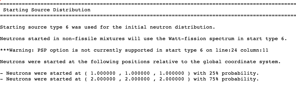
Program verification information Fig. 2.2.4 is printed after the header page. It lists the name of the program, the date the load module was created, the library that contains the load module, the computer code name from the configuration control table, and the revision number. The job name, date, and time of execution are also printed. This information may be used for quality assurance purposes.

Fig. 2.2.4 Sample program verification table.

2.2.6.1.2. General problem information

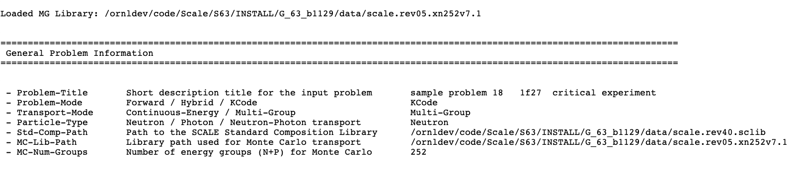
A general problem information output edit, shown in Fig. 2.2.5, follows the program verification information table. This table is printed by all SCALE Shift sequence implementations. After printing the title given in the input, it summarizes some high-level information for the physics setup of the Shift code.

Fig. 2.2.5 Sample general problem information table.

2.2.6.1.3. Input Warnings

CSAS-Shift captures the warning messages emitted from the ExnihiloInputBuilder when processing KENO data for the Shift transport. All these stacked warning messages are printed in the input warnings output table as shown in Fig. 2.2.6.

Fig. 2.2.6 Sample input warnings table.

2.2.6.1.4. Tables of parameter data

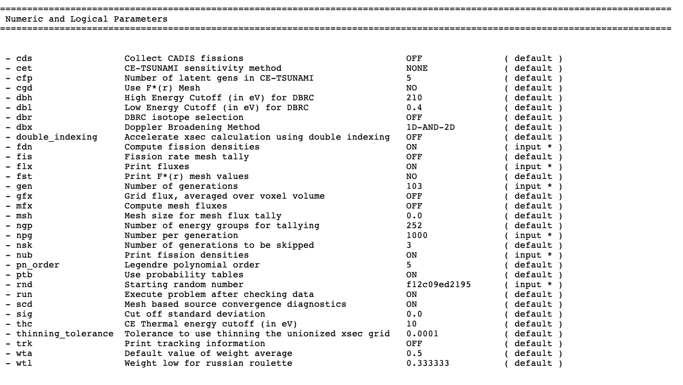
The CSAS-Shift parameter edits list both numeric and logical parameters in the same table. In each table row, the name of the KENO parameter, its short description, the current value of the parameter, and its input method are printed. If the parameter value has been entered by user in the KENO parameter data block, the input method is printed as ( input * ). Otherwise, the input method is printed as ( default ). The user should always verify that the parameter data block was entered as desired. An example of the parameters table is shown in Fig. 2.2.7.

Fig. 2.2.7 Sample table of numeric and logical parameter data.

2.2.6.1.5. Energy boundaries data

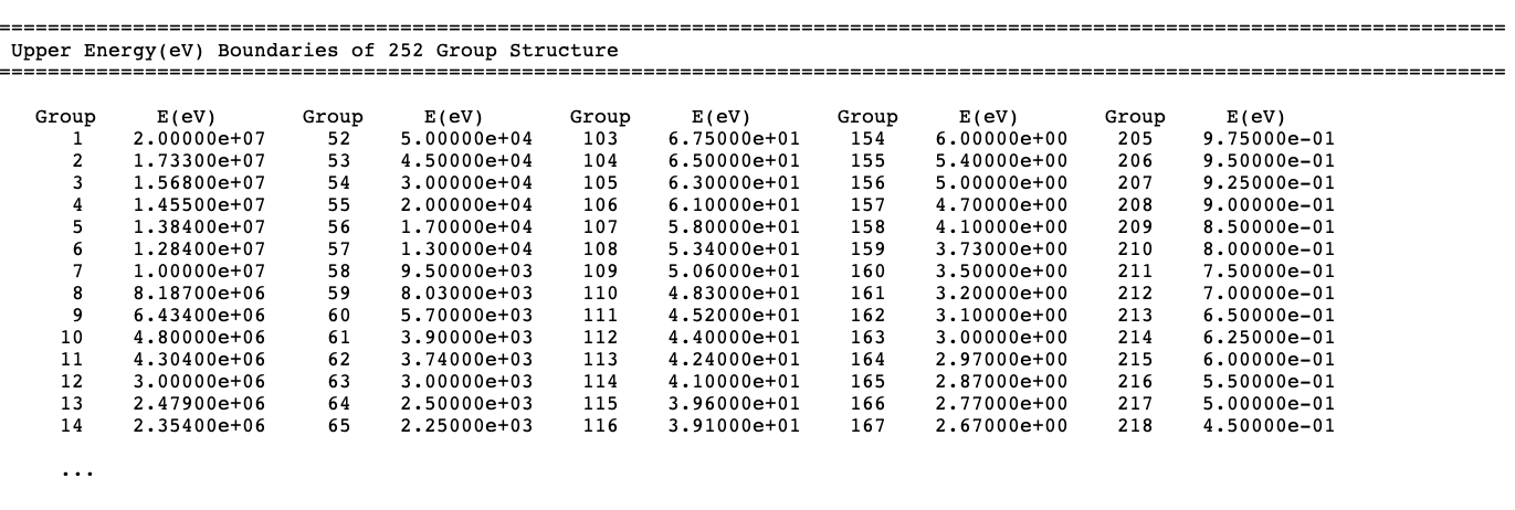
The CSAS-Shift implementation supports multiple sets of energy boundaries specifications for some of the tallies. This can be done by using the definitions data block as described in the CSAS manual Sect. 2.1.4. However, it prints only the default energy group bounds in the energy boundaries data edit, as illustrated in Fig. 2.2.8. Energy group boundaries used for each mesh tally will be printed in the mesh tallies output edit.

Fig. 2.2.8 Sample energy boundaries edit.

2.2.6.1.6. Mixing table data edits

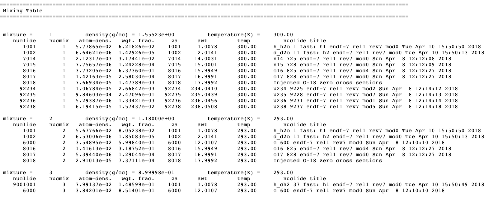
CSAS-Shift uses the same format and contents as those described for KENO codes in Sect. 8.1.3.10 for the mixing table data edits. In this table, the mixture number, density, and temperature are first printed, followed by a table of the nuclides which make up the mixture. This table contains the following data: nuclide ID number, nuclide mixture ID number, atom density, weight fraction of nuclide in mixture, ZA number, atomic weight, temperature, and nuclide title. Mixture temperature is the same as the nuclides’ temperatures for the multigroup calculations, but it may show some differences in continuous-energy calculations. See Sect. 8.1.3.10 for details.

A sample mixing table data edit is shown in Fig. 2.2.9 for a multigroup calculation.

Fig. 2.2.9 Sample mixing table edit.

2.2.6.1.7. Geometry data edits

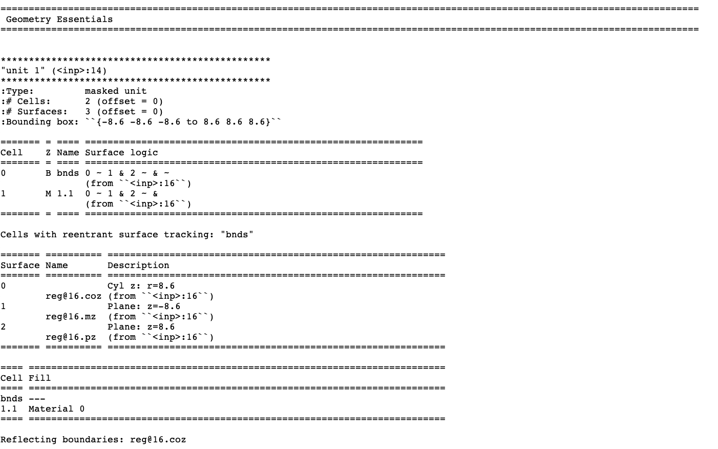
CSAS-Shift captures the output edit from ORANGE and prints these data as the overview of the geometry. Its format is completely different from the traditional KENO geometry output format but includes more descriptive sections for each geometry piece, as shown in Fig. 2.2.10.

Fig. 2.2.10 Sample ORANGE geometry output edit.

2.2.6.1.8. Volume information

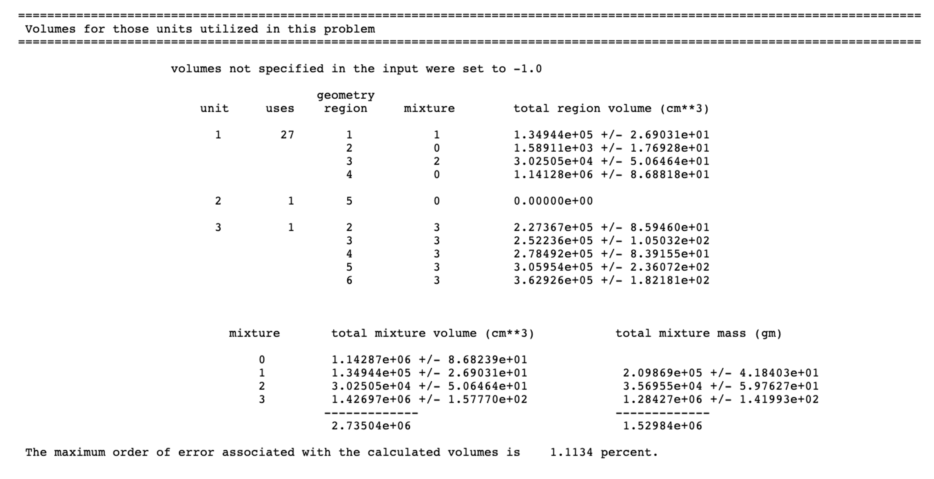
Volume tables for both KENO V.a and KENO-VI geometries are always printed by CSAS-Shift using the KENO-style volume editing format and cannot be suppressed. KENO V.a and KENO-VI volume tables show some differences, and all these details are described in KENO manual. See Sect. 8.1.5.17 for further details.

A sample volume output edit for KENO-VI geometry printed by CSAS-Shift is shown in Fig. 2.2.11.

Fig. 2.2.11 Sample volume output edit.

2.2.6.1.9. Initial source edits

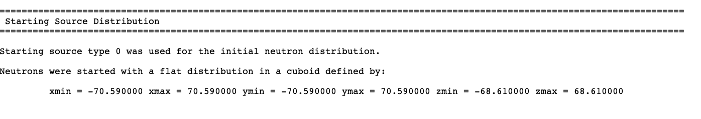
A summary table is always printed for start types 0, 1, 6, 7, and 8. The table format is the same for both KENO V.a and KENO-VI geometries. Fig. 2.2.12 illustrates typical starting data for start type 0. The parameter used in this example was NST=0.

Fig. 2.2.12 Example of start data.

2.2.6.1.10. K-effectives by generation

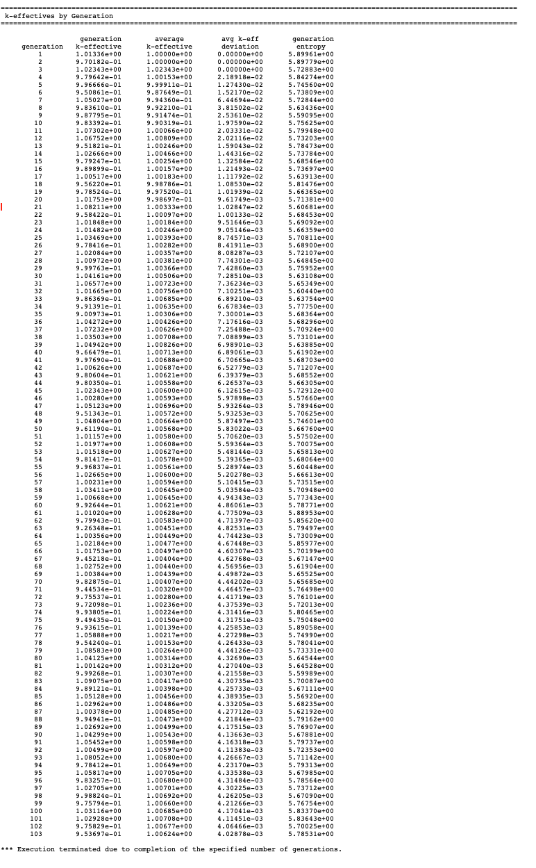
At the completion of each generation, CSAS-Shift prints the k-effective for that generation and associated information obtained from the Shift transport module. An example of this printout is given in Fig. 2.2.13.

Fig. 2.2.13 Example of k-effectives and source entropy by generation.

The data printed include (1) the generation number, (2) the k-effective calculated for the generation, (3) the average value of k-effective through the current generation (excluding the nskip - 1 generations), (4) the deviation associated with the average k-effective, and (5) Shannon entropy for the generation.

After the last generation, a message is printed to indicate why execution was terminated. The user should examine this portion of the printed results to ensure that k-effective is in acceptable agreement and to verify that the average value of k-effective has become relatively stable. If the k-effectives appear to be oscillating or drifting significantly, then the user should consider rerunning the problem with a larger number of histories per generation.

Note

k-effective values from Shift calculations are always printed to the standard output (and .msg file). There is no user option to suppress this.

2.2.6.1.11. Problem characterization edit

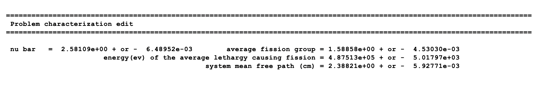
The problem characterization edit follows the k-effective by generation edit. The average number of neutrons per fission, NU BAR, and its associated deviation are printed, and the AVERAGE FISSION GROUP (the average energy group at which fission occurs) and its associated deviation are printed at the top of this edit. Then the ENERGY (eV) OF THE AVERAGE LETHARGY OF NEUTRONS CAUSING FISSION and its associated deviation are printed, followed by the system mean free path. A typical problem characterization edit is shown in Fig. 2.2.14.

Fig. 2.2.14 Example of problem characterization edit.

Note

lifetime and generation time are not currently available with Shift transport.

2.2.6.1.12. Final k-effective edit

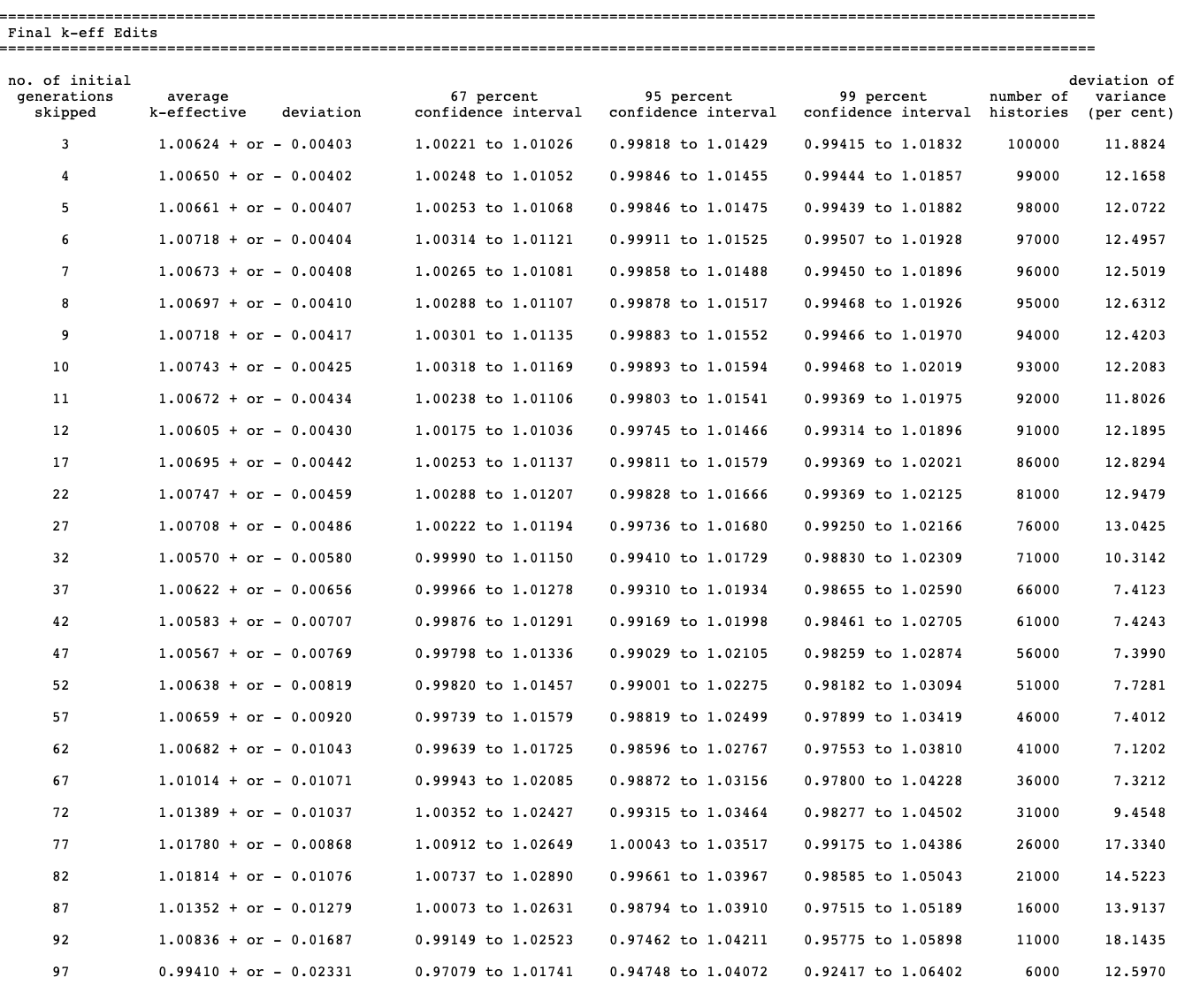
The final k-effective edit prints the average k-effective, its associated deviation, and the limits of k-effective for the 67, 95, and 99% confidence intervals. The number of histories used in calculating the average k-effective is also printed. This is done by skipping various numbers of generations. The user should carefully examine the final k-effective edit to determine whether the average k-effective is relatively stable. If a noticeable drift is apparent as the number of initial generations skipped increases, then it may indicate a problem in converging the source. If this appears to be the case, the problem should be rerun with a better initial source distribution and should be run for sufficient number of generations so that the average k-effective becomes stable. The final k-effective edit is printed as shown in Fig. 2.2.15.

Fig. 2.2.15 Example of the final k-effective edit.

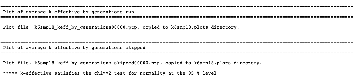
2.2.6.1.13. Plot of average k-effective by generations run and by generations skipped

ASCII character plots of the average k-effective versus the number of generations run, and the average k-effective versus the number of generations skipped, are not printed by CSAS-Shift in the code output. Instead, two Ptolemy plot files are created and copied into the plots directory in ${OUTDIR}. The name of the plot files and their final destinations are printed in the output, followed by the final k-effective edit as illustrated in Fig. 2.2.16. These plot files can be loaded and visualized by Fulcrum using the display convergence plots capability.

Fig. 2.2.16 Information about the average k-effective plot files.

2.2.6.1.14. Shannon Entropy Diagnostics

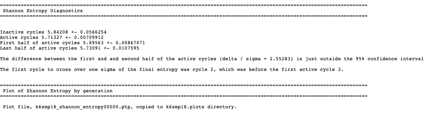
CSAS-Shift does not perform any posterior entropy tests like those available in KENO codes. Instead, it captures diagnostic test results performed by Shift and prints its details in the Shannon entropy diagnostics output edit, as shown in Fig. 2.2.17

Fig. 2.2.17 Sample Shannon Entropy Diagnostics edit.

2.2.6.1.15. Fission densities

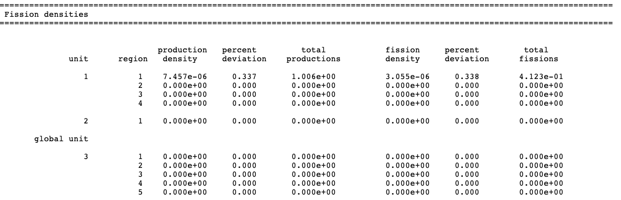
The fission density edit is optional. CSAS-Shift prints the neutron production density and the fission density for each geometry region if parameters FDN=YES and NUB=YES are specified in the parameter data (these are the default values). If NUB=NO is specified but FDN=YES, then only the production density will be given. An example of the fission density edit is shown in Fig. 2.2.18

Fig. 2.2.18 Example of the fission density edit.

2.2.6.1.16. Flux Edit

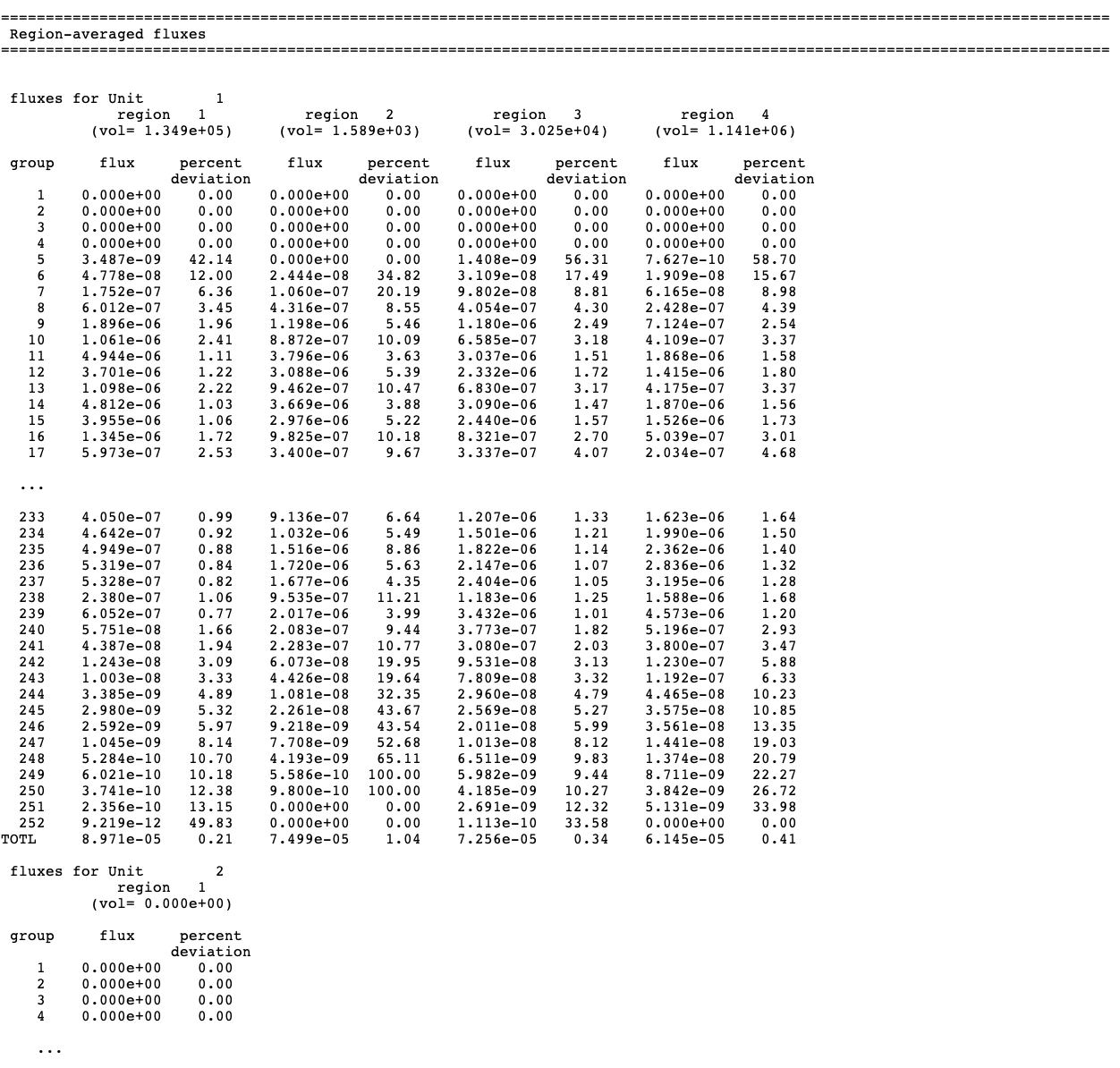
Printing the fluxes is optional; they are printed only if FLX=YES is specified in the parameter data. The fluxes are printed for each unit and each geometry region in the unit for every energy group. A sample of a flux edit is given in Fig. 2.2.19.

Fig. 2.2.19 An example of a flux edit.

2.2.6.1.17. Mesh tallies

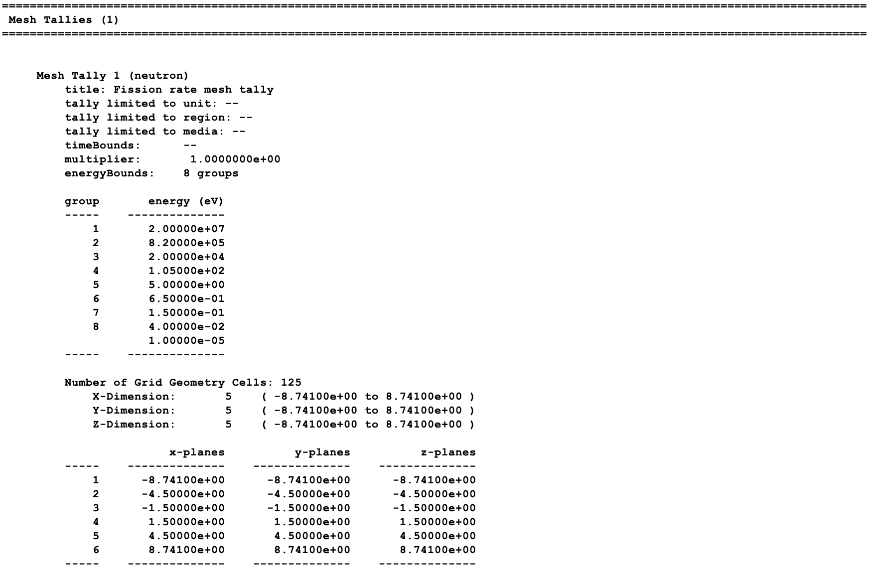
The mesh tallies edit is optional. CSAS-Shift prints the specification of each mesh tally either defined by CDS=, FIS=, and GFX= parameters or a mesh tally input block in the tallies data block. A sample mesh tallies edit is given in Fig. 2.2.20.

The number of tallies computed for the given problem is printed just after the mesh tallies edit title. Then, a summary section including the tally title and multiplier is provided. A summary of the energy and spatial grids is presented after this section.

Fig. 2.2.20 An example of mesh tallies edit.

2.2.6.1.18. Mesh tally files

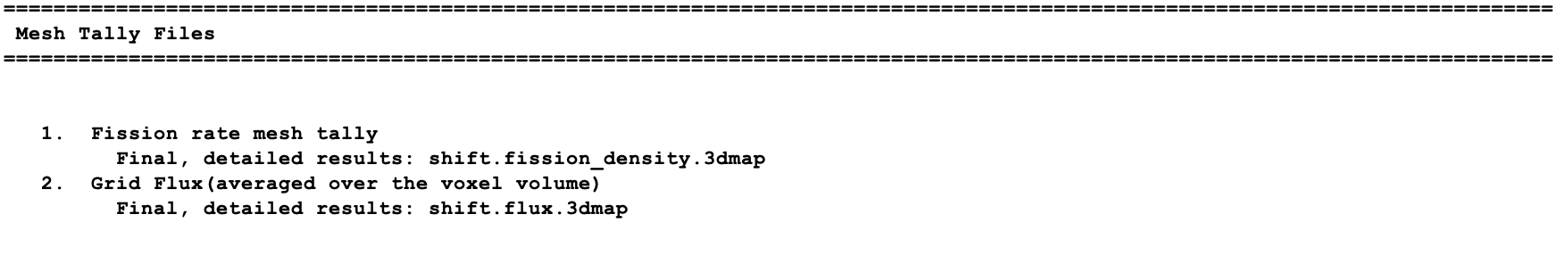
The mesh tally files edit is optional. CSAS-Shift stores the mesh tally results in MeshFile format in 3dmap files, and this output summarizes the mesh tally and corresponding 3dmap filename as depicted in Fig. 2.2.21.

Fig. 2.2.21 An example of mesh tally files edit.

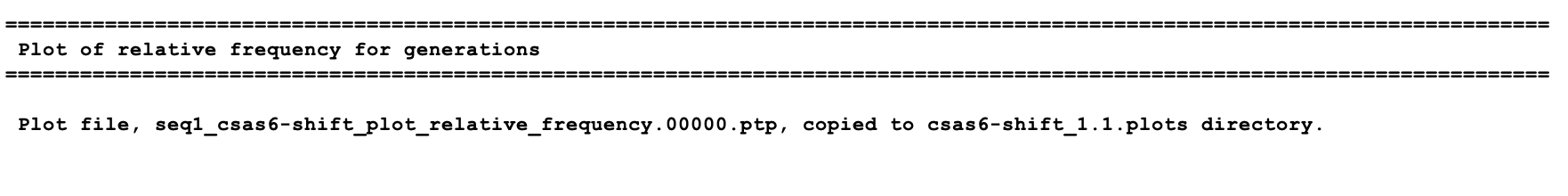
2.2.6.1.19. Plot of relative frequency distributions

A relative frequency distribution consists of a bar graph indicating the normalized number of generations that have k-effective in a specified interval. The intervals are determined by the code, based on the upper and lower limits of the k-effectives calculated for the generations. A relative frequency distribution plot includes the following bar graphs: (1) all active generations, (2) the last 3/4 of active generations, (3) the last half of active generations, and (4) the last quarter of active generations. Note that departures from normal distributions in these plots and radical shifts among them may be indications of source convergence issues in the calculation.

A Ptolemy plot file is created and copied into the ${BASENAME}.plots directory in ${OUTDIR}. The name of the plot file and its final destination are printed in the output, in the plot of relative frequency distributions edit as illustrated in Fig. 2.2.22. The plot file can be directly visualized by Fulcrum’s display convergence plot capability.

Fig. 2.2.22 Information about the relative frequency distributions plot file.

2.2.6.1.20. Final results table

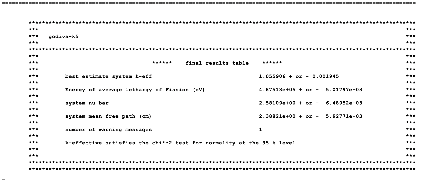
The final results table contains a summary of the most important physics parameters of the system and the number of warning and error messages generated during code execution. The table contains the best-estimate system k-effective with one standard deviation, the energy of the average lethargy of fission, the average system nu-bar, the average mean free path of a neutron throughout the system, the number of warning messages generated during code execution, and a final statement on the convergence of the \(\chi^2\) test results, as shown in Fig. 2.2.23.

Fig. 2.2.23 An example of the final results table.

2.2.6.1.21. Final timing report table

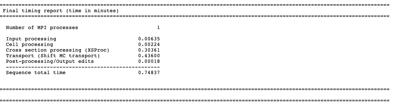
The final timing report table summarizes the time elapsed for input processing, cell processing (for multigroup mode), cross section processing (for multigroup mode), the entire transport process (Shift transport), and post-processing performed by the CSAS-Shift sequence after obtaining all results from the Shift transport calculation. A sample timing report obtained for a multigroup calculation is shown in Fig. 2.2.24.

Fig. 2.2.24 An example of the final results table.

References

[CSAS-ShiftESSC10]

Thomas M. Evans, Alissa S. Stafford, Rachel N. Slaybaugh, and Kevin T. Clarno. Denovo: A new three-dimensional parallel discrete ordinates code in SCALE. Nuclear technology, 171(2):171–200, 2010.

[CSAS-ShiftPJE+16]

T. M. Pandya, S. R. Johnson, Evans, T.M., G. G. Davidson, S. P. Hamilton, and A. T. Godfrey. Implementation, capabilities, and benchmarking of shift, a massively parallel monte carlo radiation transport code. Journal of Computational Physics, 308:239–272, 2016. Publisher: Elsevier.