9.2. NEWT: A New Transport Algorithm for Two-Dimensional Discrete-Ordinates Analysis in Non-Orthogonal Geometries
Code Responsible(s): F. Bostelmann, K. S. Kim Contributors: F. Bostelmann, K. S. Kim, D. Wiarda, M. A. Jessee
ABSTRACT
NEWT (New ESC-based Weighting Transport code) is a multigroup discrete-ordinates radiation transport computer code with flexible meshing capabilities that allow two-dimensional (2-D) neutron transport calculations using complex geometric models. The differencing scheme employed by NEWT, the Extended Step Characteristic approach, allows a computational mesh based on arbitrary polygons. Such a mesh can be used to closely approximate curved or irregular surfaces to provide the capability to model problems that were formerly difficult or impractical to model directly with discrete-ordinates methods. Automated grid generation capabilities provide a simplified user input specification in which elementary bodies can be defined and placed within a problem domain. NEWT can be used for eigenvalue, critical-buckling correction, and source calculations and it can be used to prepare collapsed weighted cross sections in AMPX working library format.
Like other SCALE modules, NEWT can be run as a standalone module or as part of a SCALE sequence. NEWT has been incorporated into the SCALE TRITON control module sequences. TRITON can be used simply to prepare cross sections for a NEWT transport calculation and then automatically execute NEWT. TRITON also provides the capability to perform 2-D depletion calculations, in which the transport capabilities of NEWT are combined with multiple ORIGEN depletion calculations to perform 2-D depletion of complex geometries. In the TRITON depletion sequence, NEWT can also be used to generate lattice-physics parameters and cross sections for use in subsequent nodal core simulator calculations.
9.2.1. Acknowledgments
The U.S. Nuclear Regulatory Commission (NRC) has been instrumental in supporting NEWT development and enhancements in each SCALE release. For SCALE 6.3 support, we express gratitude to M. Aissa (former NRC), D. Algama (former NRC), R. Y. Lee (former NRC), D. Barto, L. Kyriazidis, and H. Esmaili. Previous releases of SCALE-NEWT were funded by other government agencies and developed by several current and former ORNL staff. The original development of NEWT was led by Mark DeHart (former ORNL) who authored several sections in the current manual.
9.2.2. Introduction
NEWT (New ESC-based Weighting Transport code) is a two-dimensional (2-D) discrete-ordinates transport code developed based on the Extended Step Characteristic (ESC) approach [NEWTDeh92] for spatial discretization on an arbitrary mesh structure. This discretization scheme makes NEWT an extremely powerful and versatile tool for deterministic calculations in real-world non-orthogonal problem domains. The NEWT computer code evolved from the earlier proof-of-principle CENTAUR code [NEWTDeh92] and has been developed to run within SCALE. Thus, NEWT uses AMPX-formatted cross sections processed by other SCALE modules. If cross sections are properly prepared, NEWT can be run in stand-alone mode. NEWT can also be used within the TRITON control module for transport analysis, depletion analysis, and sensitivity and uncertainty analysis.
9.2.2.1. How to use this manual
This users’ manual is intended to assist both the novice and the expert in the application of NEWT for transport analysis. As such, the document is divided into subsections, each with a specific purpose. Not all sections will be of value to all users. It is not intended that the user of this manual read through the manual from start to end. Rather, the manual is designed to serve as a reference, with each section meeting different needs. This introductory section has been written to provide a general overview of the background, nature, functionality, and applications of NEWT; it should prove of interest to users at all levels. Sect. 9.2.3 provides detail on the theory of NEWT in terms of derivations, equations, and relationships used in the NEWT solution. This information will be of interest to those with a background in transport methods desiring a comprehensive understanding of the NEWT solution scheme. However, this information may provide too much detail or simply not be relevant for the beginning user or someone desiring to improve or expand an existing model. These users will find Sect. 9.2.4 to be of more value, where input data requirements and formats are described in detail, along with examples of each data type. This information is supplemented by Sect. 9.2.5, in which complete sample inputs with descriptions of the features of each model are provided. Sect. 9.2.6 describes the components of an output listing obtained from a successful NEWT calculation.
9.2.2.2. Background
The radiation transport equation, a linearized derivative of the Boltzmann equation, provides an exact description of a neutral-particle radiation field in terms of the position, direction of travel, and energy of every particle in the field. Both stochastic (Monte Carlo simulation) and deterministic (direct numerical solution) forms of the transport equation have been developed and are used extensively in nuclear applications. Each approach has its strengths and weaknesses. Stochastic approaches are extremely effective for problems with complex geometries where the calculations of integral quantities, such as radiation dose and neutron multiplication factors, are desired. However, calculations to obtain accurate differential information, such as the neutron flux as a function of space and energy, can be difficult and inefficient at best and prone to inaccuracies (even if the integral quantity is correct). Deterministic techniques, such as integral transport, collision probability, diffusion theory, and discrete-ordinates methods, are better suited for problems where differential quantities, such as the neutron flux as a function of energy or space, are desired. However, integral transport, collision probability, and diffusion approximations are based on simplifying assumptions, which can limit their applicability. The discrete-ordinates approach is a more rigorous approximation to the transport equation but is typically very limited in its flexibility to describe complex geometric systems.
Discrete-ordinates approaches are derived from the integro-differential form of the Boltzmann transport equation, where space, time, and energy dependencies are normally treated by the use of a finite-difference grid, while angular behavior is treated by considering a number of discrete directions in space. The angular solution is coupled to a scalar spatial solution via some form of numerical integration. Because of the direct angular treatment of the discrete-ordinates approach, angularly dependent distribution functions can be computed; thus, this approach is the preferred method of solution in many specific applications where angular anisotropy is important. However, as indicated earlier, it is often limited in applicability because of the geometric constraints of the orthogonal grid system associated with the finite-difference numerical approximation.
9.2.2.3. Discrete-ordinates solution on an arbitrary grid
The ESC approach was developed to obtain a discrete-ordinates solution in complicated geometries to handle the needs of irregular configurations. Deterministic solutions to the transport equation generally calculate a solution in terms of the particle flux; the flux is the product of particle density and speed and is a useful quantity in the determination of reaction rates that characterize nuclear systems. General 2-D xy discrete-ordinates methods perform calculations that provide four side-averaged fluxes and a cell-averaged flux for each cell in a rectangular problem grid; iteration is performed to obtain a converged distribution. This approach is usually termed the diamond-difference approach. Using the ESC approach, a more flexible and completely arbitrary problem grid may be defined in terms of completely arbitrary polygons. Side-averaged fluxes for each polygon in the problem domain are computed and are used to calculate a cell-averaged flux. This process is repeated for each cell in the problem domain, and as with the traditional approach, iteration is performed for convergence. This geometric flexibility is a significant enhancement to existing technology, as it provides the capability to model problems that are currently difficult or impractical to model directly.
9.2.2.4. Functions performed
NEWT provides multiple capabilities that can potentially be used in a wide variety of application areas. These include 2-D eigenvalue calculations, forward and adjoint flux solutions, multigroup flux spectrum calculations, and cross section collapse calculations. NEWT provides significant functionality to support lattice-physics calculations, including assembly cross section homogenization and collapse, calculation of assembly discontinuity factors (for internal and reflected assemblies), diffusion coefficients, pin powers, and group form factors. Used as part of the TRITON depletion sequence, NEWT provides spatial fluxes, weighted multigroup cross sections, and power distributions used for multi-material depletion calculations and coupled depletion and branch calculations needed for lattice-physics analysis.
9.2.3. Theory and Procedures
This section provides the theoretical basis for the ESC discretization technique, the NEWT solution algorithm, and cross section processing procedures used by NEWT. Although this information is not necessary to be able to use NEWT for transport calculations, it provides a deeper understanding of the basic operations performed within NEWT.
9.2.3.1. Boltzmann transport equation
The neutron transport equation may be presented in various forms, and simplifications are often applied to tailor the equation to the requirements of a specific application. In nuclear engineering applications, the transport equation is often written in terms of the angular neutron flux as the dependent variable. The angular neutron flux is defined as the product of the angular neutron density and the neutron velocity. The time-independent form of the linear transport equation is then expressed as [NEWTDH76]
where
\(\psi(\mathbf{r}, \Omega, E)\) \(\equiv\) angular flux at position per unit volume, in direction \(\Omega\) per unit solid angle and at energy E per unit energy;
\(\sigma_{t}(\mathbf{r}, E)\) \(\equiv\) total macroscopic cross section at position r and energy E; and
Q \(\equiv\) source at position r per unit volume, in direction \(\Omega\) per unit solid angle and at energy E per unit energy.
The source Q is generally composed of three terms:
a scattering source,
where
\(\sigma_{s}\left(\mathbf{r}, \Omega^{\prime} \rightarrow \Omega, E^{\prime} \rightarrow E\right)\) \(\equiv\) macroscopic scattering cross section at position r from initial energy E’ and direction \(\Omega\)’ to final energy E and direction \(\Omega\),
a fission source,
where
\(\sigma_{f}\left(\mathbf{r}, E^{\prime}\right)\) \(\equiv\) macroscopic fission cross section at position r and energy E’ (assumed to be isotropic),
\(v\left(\mathbf{r}, E^{\prime}\right)\) \(\equiv\) number of neutrons released per fission event at position r and energy E’,
\(\chi(\mathbf{r}, E)\) \(\equiv\) fraction of neutrons that are born at r and at energy E, and
an external or fixed source, S(r ,E).
In general, the transport equation can be difficult to apply and can be solved analytically only for highly idealized cases. Hence, simplifications and numerical approximations are often necessary to apply the equation in engineering applications. Traditional discrete-ordinates methods are based on a finite-difference approximation to solve the flux streaming (leakage) term. Such differencing schemes are intimately tied to the coordinate system in which the differencing equations are developed, and it becomes difficult to represent non-orthogonal volumes within that coordinate system. For example, it is not possible to exactly represent a cylinder in a 2-D Cartesian coordinate system; one must approximate the cylinder with a number of rectangular cells. A close approximation can require a large number of computational cells. However, the ESC approach for discretizing computational cells allows the use of non-orthogonal computational cells composed of arbitrary polygons. Using this method, practically any shape can be represented within a Cartesian grid to a very close approximation. The ESC approach is discussed in the following sections.
9.2.3.2. The step characteristic approximation
Efficient application of discrete-ordinates methods is difficult when dealing with complicated non-orthogonal geometries because of the nature of finite difference approximations for spatial derivatives. An alternative to the discrete representation of the spatial variable is achieved in the method of characteristics, in which the transport equation is solved analytically along characteristic directions within a computational cell. The angular flux is solved along the s-axis, where this axis is oriented along the characteristic direction \(\Omega\). Since only the angular flux in direction \(\Omega\) is of concern, then the streaming term can be rewritten as
Hence Eq. (9.2.1) can be written in the characteristic form (omitting E for clarity) as
which has a solution of the form [NEWTHil76]
where s is the distance along the characteristic direction \(\Omega\), and \(\psi_{0}\) is the known angular flux at s=0. The value for \(\psi_{0}\) is given from boundary conditions for known cell sides, and angular fluxes on unknown sides are computed using Eq. Eq. (9.2.6). Methods for the determination of an appropriate value for \(\psi_{0}\) and for evaluation of the integral term vary in different solution techniques.4-9 [NEWTAL81, NEWTALMJW79, NEWTHil76, NEWTLA81, NEWTLat68, NEWTLat69, NEWTLM84]. One of the simplest schemes employing the Method of Characteristics is the Step Characteristic (SC) method developed by Lathrop [NEWTAL81]. In this approach, the source Q and macroscopic total cross section \(\sigma\)t are assumed to be constant within a computational cell and the angular flux is assumed constant on the cell boundaries of incoming direction. Integration of Eq. Eq. (9.2.6) can be performed to obtain
Fig. 9.2.1 shows a sample computational cell in which the SC method can be applied. For a given characteristic direction \(\Omega\), the angular flux on any unknown side may be expressed in terms of a suitable average of fluxes from known sides, which contribute to the unknown side. For the characteristic direction \(\Omega\) shown in Fig. 9.2.1, the unknown “top” flux \(\psi_{\mathrm{T}}\) may be computed as a linearly weighted average of contributions from known sides \(\psi_{\mathrm{B}}\) and \(\psi_{\mathrm{L}}\). The fluxes on each of the two known sides are taken to be constant along the length of each side, representing the average angular flux in direction \(\Omega\) and must be specified from external boundary conditions or from a completed calculation in an adjacent cell.
The set of characteristic directions is chosen from a quadrature set, so that the resulting angular fluxes may be numerically integrated to obtain a scalar flux. Knowing the lengths of the sides of a rectangular cell (\(\Delta\)Delta`y) and the direction cosines of \(\Omega\) in the x-y plane (\(\mu\) and \(\eta\)), a function for the length s can easily be determined. The solution for from Eq. Eq. (9.2.7) can then be integrated along the length of each unknown side to determine the average angular flux of the unknown side. Once the angular flux is known on all four sides, a neutron balance on the cell can be used to determine the cell’s average angular flux.
Although the SC method described above is based on rectangular cells, the derivation of Eq. Eq. (9.2.7) makes no assumptions about the shape of the cell. It merely requires knowledge of the relationship between cell edges along the direction of the characteristic. Hence, the method is not restricted to any particular geometry. Because it is an extension of the SC approach into generalized cells, the method developed here for generalized geometries is referred to as the Extended Step Characteristic (ESC) method.
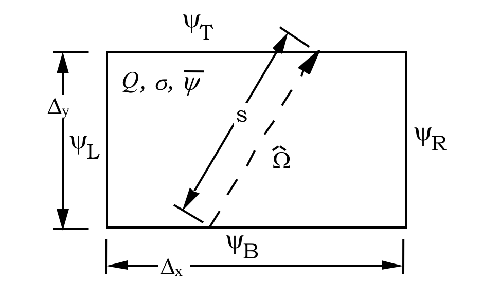
Fig. 9.2.1 Typical rectangular cell used in the step characteristic approach.
9.2.3.3. The Extended Step Characteristic approach
The theory of the ESC approach is developed and explained in detail in [NEWTDeh92]. However, the work has evolved significantly from that time, most notably in the elimination of a requirement for non-reentrant polygons (convex). The following subsections describe the primary equations applied in the ESC approach as currently applied in NEWT.
9.2.3.3.1. Cell properties and geometries
The two primary assumptions of the ESC method are that (1) within each computational cell all properties (i.e., \(\sigma\)t and Q) are uniform and (2) cell boundaries are defined by straight lines. The restriction of a computational cell to boundaries consisting of a set of straight lines results in computational cells that are limited to polygons. However, as will be seen later, no restrictions are placed on the shape of the polygon or on the number of sides in the polygon. However, the size of the polygon will be limited. In practical applications, properties are unlikely to remain constant over significant volumes. Thus this approach, like many other differencing schemes, is a poor approximation when cell volumes become too large. Although \(\sigma\)t is a material property and may remain spatially constant, the source term Q, which depends on the neutron flux, will vary with position. However, since the solution would become exact in an infinitesimally small cell, it is expected that the approximation will be reasonable for computational cells in which the change in the flux (and therefore the source) is small over the domain of the cell.
As a result of this geometric configuration, each side of a cell can have one of three possible attributes relative to particle flow in a given characteristic direction, as illustrated in Fig. 9.2.2: (1) flow can enter the cell when crossing a side (as shown by sides E and F in the figure); (2) flow can exit the cell when crossing a side (sides B and C); or (3) in a special case, flow may be parallel to the orientation of a given side (sides A and D). Expressed mathematically, these relationships become
where \(\hat{n}_{i}\) is a unit vector in the cell-outward direction normal to side i, and \(\Omega_{k}\) is the kth discrete element of a set of characteristic directions. A category 1 side will be termed an “incoming” side with respect to the direction \(\Omega_{k}\), and a category 2 side will be referred to as an “outgoing” side. For simplicity, the definition of Eq. Eq. (9.2.10) will be included as a special case of Eq. Eq. (9.2.8) for an incoming side. Thus, Eq. Eq. (9.2.8) can be rewritten as
To solve for fluxes (flow) on outgoing sides of a cell, one must know fluxes on all incoming sides. Each incoming side of each cell will be given from a boundary condition or will be the outgoing side of an adjacent cell.
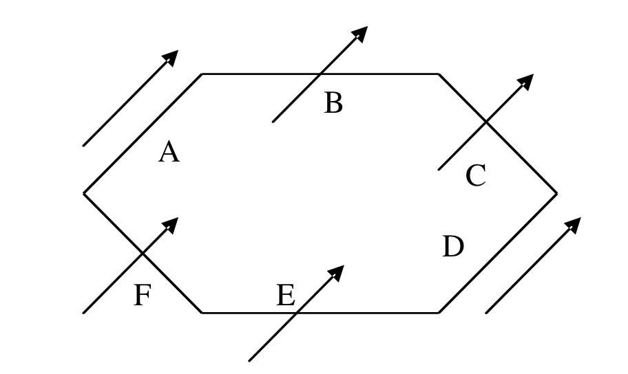
Fig. 9.2.2 Orientation of the sides of a cell with respect to a given direction vector.
9.2.3.3.2. Relationships between cells
In the ESC method, the shape of the computational cell and the form of the neutron balance differ from that used in traditional discrete-ordinates methods. Nevertheless, the relationships between cells are treated essentially as they would be in traditional approaches. The entire problem domain is mapped in terms of a set of finite cells. Each side of each cell is adjacent to either an external boundary condition or another cell. For each discrete direction, cells are swept in a predetermined order beginning at a known boundary (from a specified external boundary condition) moving in the given direction. The precise order of sweep is such that as the solution for one cell is obtained, the cell provides sufficient boundary conditions for the solution of an adjacent cell. Hence, cells sharing a given side share the value of the angular flux on that side. Knowledge of the flux on all incoming sides of a cell is sufficient to solve for all outgoing sides. Once the angular flux has been determined for all sides of the cell for the given direction, it is possible to use a neutron balance to compute the average value of the angular flux within the cell.
The sweeping of cells continues for a given direction until all cell fluxes have been calculated. The procedure is then repeated for the next direction until all directions have been computed. At this point, the cell average angular fluxes are known for each cell for each direction used. Numerical quadrature can then be used to determine the average scalar flux in each cell in the problem domain. The scalar fluxes are used to determine fission and scattering reaction rates in each cell and to update the value of the cell average source, Q. The process is repeated, and the iteration continues until all scalar fluxes converge to within a specified tolerance.
This approach can be performed assuming a single energy group or any number of discretized energy groups. The multigroup approach used in the ESC method is the standard approach used in most multigroup methods and is independent of the shape of each computational cell. Hence, the details of the multigroup formalism will be omitted from this discussion.
9.2.3.3.3. The set of characteristic directions
The characteristic solution to the transport equation gives only the angular flux in the direction of the characteristic direction vector \(\Omega_{k}\). To compute interaction rates within a cell, one must compute scalar fluxes. In computing the scalar flux from the set of angular fluxes, it is convenient to choose the set of characteristic directions from an appropriate quadrature set. Then the set of computed angular fluxes can be combined with appropriate directional weights and summed to obtain a scalar flux solution within a cell. Therefore, it is most appropriate to choose characteristic directions from an established set of base points and weights. Such quadrature sets that have been developed and used in numerous earlier discrete- ordinates approaches are used in NEWT. No restriction is placed on the nature or order of the quadrature set, as long as it is sufficient to adequately represent the scalar flux from computed angular fluxes.
9.2.3.3.4. Angular flux at a cell boundary
As in the development of the SC method, as well as most finite-difference methods, the ESC approach does not explicitly determine the flux distribution as a function of position along the sides of a computational cell. Instead, the angular flux on each cell side is represented in terms of the average angular flux along the length of the side. This is sufficient to determine the net leakage across each cell side, which is needed in order to maintain a cell balance. An average value of the flux for an incoming side must be specified from a boundary condition or from the prior solution of an adjacent cell. The average flux along a given outgoing side can be computed by integrating the flux along the side and dividing by the length of the side. However, the form of the distribution of the angular flux on the side must be known to perform this integration. This distribution can be determined from the properties of the cell and from the average flux on each of the known incoming sides.
Because the characteristic solution [Eq. Eq. (9.2.6)] allows calculation of the angular flux at any point s in a single cell given an initial condition, the exact value of the flux can be computed at any point on any outgoing side if the flux along each incoming side is known. As an initial condition, it is assumed that the angular flux in some characteristic direction is known at some starting point, s = 0 [i.e., \(\psi(0)=\psi_{0}\)], on an incoming side. To determine the flux at some point on an outgoing side, one need know only the distance s measured along a characteristic direction to the appropriate incoming side. This method can then be expanded to determine a functional form of the flux for every point on the outgoing side, which can be integrated to produce the average outgoing flux on the side.
To develop a mathematical relationship between two arbitrary sides of a cell, one should first consider two arbitrary coplanar line segments in space whose endpoints each lie on a pair of parallel lines laid in the direction \(\Omega_{k}\), as shown in Fig. 9.2.3. Points B1 and B2 can be considered to be the “projections” of A1 and A2, respectively, relative to \(\Omega_{k}\). Because s is the distance between a point on segment A and its projection on segment B, it can be seen that s varies linearly in moving from the “beginning” to the “end” of the pair of segments.
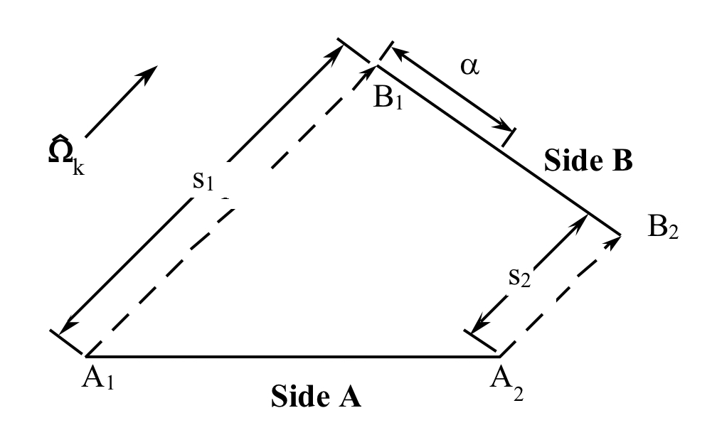
Fig. 9.2.3 Line endpoints for computation of average fluxes.
If \(\alpha\) is the distance along segment B measured from endpoint B1 and B has a total length L, then the distance s between A and B along direction \(\Omega_{k}\) can be written as a linear function in terms of the position \(\alpha\):
where s1 and s2 are related to the distances along the characteristic direction between A1, B1 and A2, B2, respectively. (It is important to note that the length s is the same as the distance between the endpoints only when the characteristic vector lies in the plane of the computational cell. This is not necessarily the case, depending on the choice of quadrature directions. This situation is discussed in more detail later.)
If \(\psi(\alpha)\) is the angular flux on side B at a distance \(\alpha\) from B1, then \(\bar{\psi}_{\mathrm{B}}\), the average value of \(\psi\) on B, is given by
Equation Eq. (9.2.6), the solution to the characteristic equation in the step approximation, can be rewritten in terms of the average known angular flux on side A
Inserting Eqs. Eq. (9.2.13) and Eq. (9.2.15) into Eq. Eq. (9.2.14) and simplifying yields
For the special case in which A and B are parallel, s1 = s2 and the second term in the exponential drops out. Equation Eq. (9.2.16) can easily be integrated to obtain
In the more general case, s1 \(\neq\) s2, the result is slightly more complicated:
Equations Eq. (9.2.17) and Eq. (9.2.18) can also be written in a simplified form:
where
(9.2.20)\[\begin{split}\beta_{A B}=\left\{\begin{array}{cc} \frac{e^{-\sigma_{t} s_{1}}-e^{-\sigma_{t} s_{2}}}{\sigma_{t}\left(s_{2}-s_{1}\right)} & s_{1} \neq s_{2} \\ e^{-\sigma_{t} s_{1}} & s_{1}=s_{2} \end{array}\right.\end{split}\]
Thus far, this development has considered only the special case where contributions to side B are the result only of the cell internal source and a single incoming side (i.e., side A). For an arbitrarily shaped cell and discrete direction \(\Omega_{k}\), it is likely that the outgoing side would receive contributions from two or more incoming sides, as illustrated in Fig. 9.2.4, for a cell with three incoming sides (X, Y, and Z) contributing to the flux on a single outgoing side (B). In such a situation, the outgoing side can be subdivided into multiple components. Side B of Fig. 9.2.4 can be represented by three components, BX, BY, and BZ, representing contributions from line segments X, Y, and Z, respectively. The average angular flux \(\bar{\psi}\) can be computed for each component of side B using Eq. Eq. (9.2.19); then \(\bar{\psi}_{B}\), the average flux for the entire length of B, can be calculated by the length-weighted average of each component. In general, for a given side B composed of n components, the average flux of the side is given by
where
\(\ell_{i}\) is the length of the projection of the ith side onto B, and
\(\bar{\psi}_{i}\) is the average flux computed for segment Bi due to the flux on side i
Using Eqs. Eq. (9.2.19) and Eq. (9.2.21), one can compute the average flux on each of the outgoing sides for a given cell, once the angular flux on each incoming side is known. At this point, only distances s1 and s2 and the lengths \(\ell_{i}\) and L need be determined to estimate fluxes in an iterative process. These can be computed from the geometry of the cell and the direction \(\Omega_{k}\).
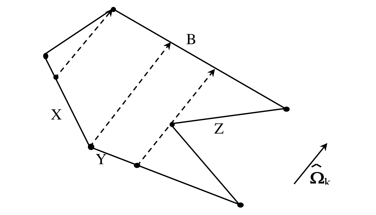
Fig. 9.2.4 Contributions of multiple incoming sides to an outgoing side.
9.2.3.3.5. Mapping a characteristic vector into the two-dimensional problem domain
Even in a 2-D x-y system in which the scalar flux is constant with respect to the z axis, the angular flux has components in the z direction. Thus, to obtain the scalar flux at a point on the x-y plane, one must integrate over the unit sphere in all \(4 \pi\) directions of \(\Omega\). Recall that the choices of characteristic directions for this model were selected to be the same as the set of directions composing a conventional quadrature set. Quadrature sets specified in the literature [NEWTCL65, NEWTCar70, NEWTLee62] and used in other discrete-ordinates codes [NEWTEJ67, NEWTLB73] are based on a unit sphere and are usually specified in terms of \(\mu_{\mathrm{k}}\) and \(\eta_{\mathrm{k}}\), the respective x and y components of \(\Omega_{k}\), where is one of a set of discrete directions composing the quadrature set. Because \(\Omega_{k}\) is a unit vector, \(\xi_{k}\), the z component of the direction, is implicit: \(\xi_{k}=\sqrt{1-\mu_{k}^{2}-\eta_{k}^{2}}\). However, because of the 2D nature of the problem, the z component is never explicitly used. It is therefore sufficient to evaluate the angular flux at a finite number of points in \(4 \pi\) of \(\Omega\)-space in terms of just the \(\mu_{\mathrm{k}}\) and \(\eta_{\mathrm{k}}\) components of the discrete directions \(\Omega_{k}\). One must recognize, however, that the length of the path traveled by particles moving in a direction out of the x-y plane is always longer than the x-y projection of the path, by a factor of \(\left(\mu^{2}+\eta^{2}\right)^{-1 / 2}\). Thus, for any path length s’ measured in the x-y plane for a given direction \(\Omega_{k}\), the true path length traveled is s, where
This is illustrated in Fig. 9.2.5.
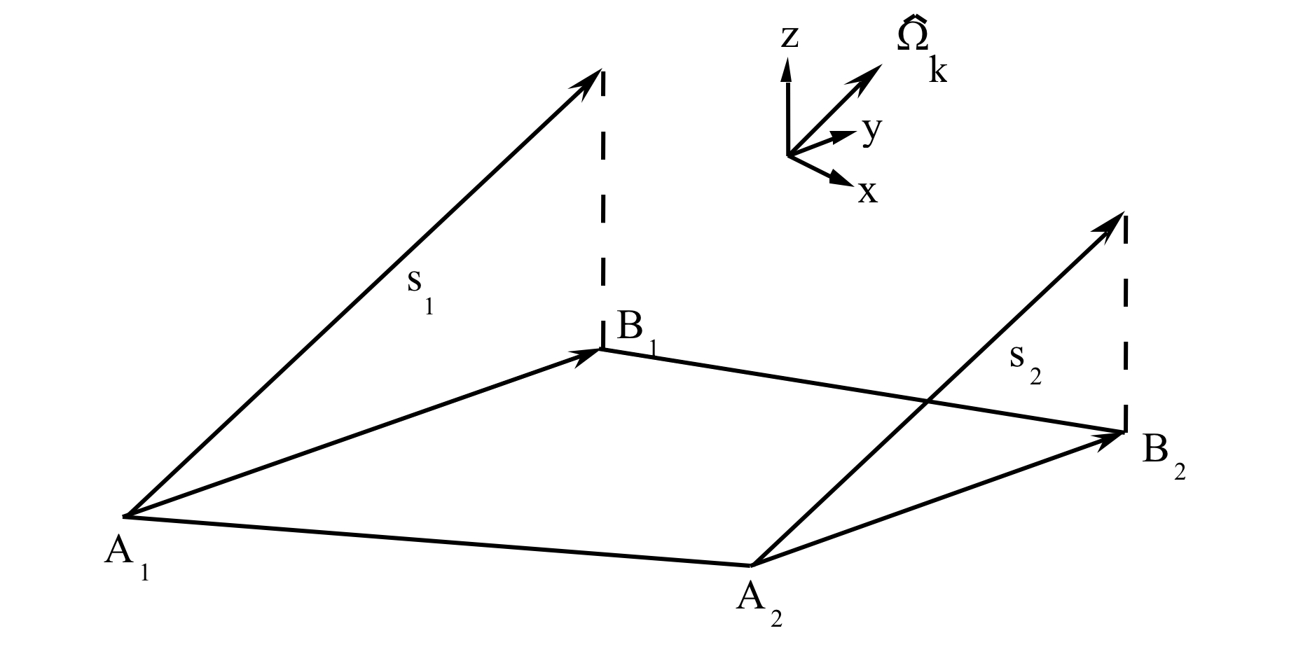
Fig. 9.2.5 Relationship between s1 and s2 and their projections in the x-y plane.
9.2.3.3.6. Neutron balance within a computational cell
Once angular fluxes have been computed for all sides of a cell, it is necessary to compute the cell-averaged angular flux. To enforce conservation, a balance condition is applied to the cell. This provides the equation necessary to determine the average flux in the cell. The neutron balance for an arbitrary cell in steady state may be expressed as
or, expressed mathematically,
where \(n\) is the outward normal direction at each side of the cell and V is the 2-D volume of the cell. Note that in this context, S represents the surface area or perimeter of the cell. Hence, for a cell with m sides, each of the sides having a constant angular flux \(\bar{\psi}_{i}\) and an outward normal direction \(\mathrm{n}_{i}\),
Because each cell is restricted to be a polygon, each side in the cell will be a straight line and \(\mathrm{n}_{i} \cdot \hat{\Omega}_{k}\) will be constant along the length of the side. Equation Eq. (9.2.25) can then be simplified to obtain
where Li is the length of the ith side and the term in parentheses represents a leakage coefficient for the side.
9.2.3.4. Coarse-mesh finite-difference acceleration
Beyond cell discretization and solution described above for the ESC approach, the NEWT iterative approach is similar to that used in other discrete-ordinates methods. Inner iterations are used to solve spatial fluxes in each energy group to generate updated source terms; outer iterations use these source terms to converge all energy groups. This source-iteration approach can be somewhat slow to converge, especially when significant scattering is present. Hence, it is desirable to apply some form of acceleration to the iterative solution used by NEWT. To this end, a coarse-mesh finite-difference acceleration (CMFD) approach has been added to NEWT. The CMFD formulation uses a simplified representation of a complex problem, in which selected rectangular regions are derived from the global NEWT Cartesian grid and homogenized. The CMFD formulation utilizes coupling correction factors for each homogenized cell to dynamically homogenize the constituent ESC-based polygonal cells during the iterative solution process such that the heterogeneous transport solution can be preserved. Dynamic-group collapse is also possible with a two-level CMFD formulation in which alternating multigroup and two-group calculations are performed. By extending the concept of the equivalence theory to energy and angle, it is possible to apply a consistent lower-order formulation in the form of a homogenized pin-cell, few-group, diffusion-like finite-difference scheme. This simplified lower-order formulation is much less expensive to solve, and its solution can be used to accelerate the original higher-order transport solution in NEWT, resulting in much faster convergence of the fission and scattering source distributions. This work is described in detail in [NEWTZDX+08] and in previous versions of the NEWT manual.
Although the original implementation of the CMFD acceleration method is extremely efficient and actively maintained, its use is limited to rectangular-domain configurations (e.g., square-pitched fuel lattices). An alternative CMFD acceleration method has been developed to support triangular- and hexagonal-domain configurations (e.g., triangular-pitched fuel lattices such as the VVER or prismatic graphite models). The new CMFD acceleration method does not require the coarse-mesh cells to be rectangles but rather arbitrary polygons. However in the current implementation, the “unstructured” coarse-mesh cells are still constructed from the global NEWT Cartesian grid. Therefore, for a hexagonal configuration, interior coarse-mesh cells will be rectangular shape whereas cells near the boundary will be triangular or trapezoidal shapes.
The new unstructured CMFD iterative solution scheme is essentially identical to the original solution scheme; the two methods differ only in how the lower-order system is solved. Additionally the two-group acceleration is not employed in the unstructured CMFD method. Input options for both CMFD methods are described in Sect. 9.2.4.2.
9.2.3.5. Assembly discontinuity factors
In nodal multi-assembly or core calculations, lattice transport solutions are used to generate few-group homogenized cross sections. These cross sections are in general obtained from single-assembly transport calculations with zero-current boundary conditions. Generation of few-group homogenized cross sections for nodal calculations typically includes the generation of discontinuity factors (i.e., additional parameters used to preserve both reaction rates and the interface currents in the homogenization process). The discontinuity of the flux at an assembly interface that can arise by the use of homogenized cross sections is illustrated in Fig. 9.2.6. The so-called “homogeneous” flux, computed in the nodal calculation, is discontinuous at the assembly interface, as opposed to the exact “heterogeneous” flux, computed in the transport calculation, which is continuous at the assembly interface. The interface condition employed in nodal calculations between two assemblies (nodes) i and i+1 is given as
where \(F_{i}^{+}\) and \(F_{i+1}^{-}\) are assembly discontinuity factors (ADFs) on each side of the interface between assemblies i and i+1.
The ADF on the assembly interface is defined as the ratio of the heterogeneous flux \(\phi_{\text {heterogeneous }}\) at that assembly interface to the homogeneous flux evaluated at the interface, denoted \(\phi_{i, \text { homogeneous }}^{+}\) (or \(\phi_{i+1, \text { homogeneous }}^{-}\)):
Fluxes, and therefore ADFs, vary with energy; therefore, few-group homogenized cross sections are always accompanied by corresponding few-group ADFs.
In a single-assembly calculation with zero-current boundary conditions, the heterogeneous flux at each boundary is easily calculated as the surface-averaged scalar flux on the boundary, whereas the homogenous flux at each boundary is simply the assembly-averaged flux. Hence, for each energy group, the ADF is calculated for each boundary as the ratio of the average flux on that boundary to the average flux across the assembly.
In other configurations, such as a multi-assembly calculation or an assembly located on the edge of a core next to the core baffle and reflector, the ADF calculation requires more effort. For reflector situations, NEWT applies a simple one-dimensional (1-D) multigroup diffusion approximation to determine the ADF at the assembly boundary. In this approximation, it is assumed that the reflector is infinite and that the scalar flux goes to zero at infinity. The reflector ADF can be determined analytically using this boundary condition along with the known surface-averaged current and scalar flux evaluated at the assembly/reflector interface.
The reflector ADFs computed by NEWT may potentially be different from the ADFs calculated using the diffusion approximations employed by the nodal code. Moreover, ADFs computed for multi-assembly or hexagonal-domain configurations will depend on the nodal method employed. For these reasons, NEWT supports the option to edit surface-averaged scalar flux and current values along user-defined line segments so that appropriate ADFs can be computed directly by the nodal code. The input options for the single-assembly ADF, reflector ADF, and arbitrary line-segment edit are discussed in Sect. 9.2.4.11.
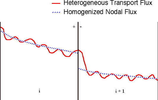
Fig. 9.2.6 Heterogeneous vs homogeneous fluxes in a multi-assembly solution.
9.2.4. Input Formats
NEWT input is free form and keyword based, similar in form to the input for many other modules in the SCALE code package. Input may start with a title card record, but this line may be omitted if desired; remaining data are supplied in data blocks. The order of the data blocks is arbitrary (with two exceptions), and many blocks are optional. Only one instance of a data block is allowed.
9.2.4.1. Overview of newt data blocks
The NEWT input deck data blocks are defined by keyword delimiters in the following form:
read keyword [data] end keyword
Read routines are terminated by the “end keyword” label, and any intervening carriage returns or line feeds are ignored. Thus, data can also be entered in this format:
read keyword
[data]
[data]
end keyword
Within each block, specific control or specification parameters are input. Each block contains a fixed set of input parameters (also defined by keyword).
As with other keyword-driven modules within SCALE, lines beginning with a single quote (‘) in the first column are treated as comments and ignored.
The keyword name and general contents of each data block are as follows:
Block type |
Recognized keywords |
Description |
Problem control parameters |
parameter, parameters, param, parm, para |
General problem parameters-must follow title card, if used (optional) |
Material properties |
material, materials, matl |
Assigns characteristics (e.g., Pn scattering order and material description) for each material ID-must follow problem control block or must follow title card if control block is omitted (required) |
Broad group collapse |
collapse, coll |
Defines broad group energy ranges to be created from the original fine group library when cross section collapse is desired (optional) |
Simple-body geometry |
geometry, geom |
Defines basic grid structure and all bodies to be placed within this structure (required unless geometry restart file is available) |
Boundary conditions |
bounds, bnds |
Defines boundary conditions to be applied on outer boundaries of global unit (optional, default is reflective on all sides) |
Array specifications |
array |
Defines composition of all arrays (unit placement within each array). Each array placed within the geometry block must be defined in the array block |
Homogenization instructions |
homog, hmog, homo |
Defines mixtures to be flux weighted and homogenized in the preparation of a homogenized cross section library (optional) |
Assembly discontinuity factors |
adf |
Assigns type and location of planes at which assembly discontinuity factors (ADFs) are calculated (optional) |
Flux plane |
flux |
Allows definition of an x- or y-axis line (plane) for which average fluxes are computed and printed (optional) |
Mixing table |
mixtable, mixt |
Mixing table specification (optional) |
Source definition |
src, source |
Defines particle source strength for use in source calculations |
Each of the following subsections describes the parameters associated with a specific data block, lists default values (if available), and describes meaning of the parameter and its effect on a NEWT calculation.
9.2.4.2. Parameter block
Parameter Block keyword = param, parm, para, parameter, or parameters
The Parameter block contains problem control parameters and must come immediately after the title card if one is used. Valid parameter specifications are described below. For each keyword, allowable values are listed in parentheses, and the default (if any) is listed in brackets. Input that can take an arbitrary integer value is indicated by an IN; similarly, any parameter that can take an arbitrary real/floating point value is indicated by RN as the allowable value. However, note that SCALE read routines do allow input of integers for real numbers, and vice versa; the number will be converted accordingly. The order of the parameters within the block is arbitrary, and may be skipped if a default value is desired for that parameter. Control parameters are set in the order in which they are input; this means that the same parameter may be listed multiple times, but only the final value is used.
9.2.4.2.1. Convergence and acceleration parameters
epseigen=(RN) - Convergence criterion for keff. [0.0001]
epsinner=(RN) - Spatial convergence criterion for inner iterations. [0.0001]
epsouter=(RN) - Spatial convergence criterion for outer iterations. [0.0001]
epsthrm=(RN) - Spatial convergence criterion for thermal-upscattering iterations, if enabled. [same value as epsouter]
epsilon=(RN) - Simultaneously sets all (spatial and eigenvalue) convergence criteria to the same value. [uses individual defaults]
converg=(cell/mix) - Sets the region within which convergence testing is applied. Use of cell will force converged scalar fluxes in every computation cell, while mix will relax convergence such that averaged scalar fluxes within a mixture are converged. The latter is useful for mixtures in which fluxes become very small-large reflectors or near a vacuum BC. [cell]
therm=(yes/no) - Enables/disables thermal-upscattering iterations. [yes]
inners=(IN) - Maximum number of inner iterations in an energy group. [5]
therms=(IN) - Maximum number of thermal-upscattering iterations, if enabled. [2]
outers=(IN) - Maximum number of outer iterations. NEWT will stop with an error code if more than outers outer iterations are required for convergence. [250]
inrcvrg=(yes/no) - If inrcvrg=yes, NEWT will continue outer iterations until all convergence criteria are met. If inrcvrg=no, NEWT will stop whenever outer iteration and keff convergence criterion are met, regardless of the convergence of inner or thermal-upscattering iterations. [no]
cmfd=(no/rect/yes/part) - CMFD acceleration option. If cmfd=no, CMFD acceleration is not employed. If cmfd=rect, the CMFD method is employed. The original NEWT CMFD method can be applied only to rectangular-domain configurations. If cmfd=yes, the unstructured CMFD method is employed. The new unstructured CMFD method can be applied to rectangular-, triangular-, and hexagonal- domain configurations. If cmfd=part, an alternative version of the unstructured CMFD method is employed and uses a “partial-current” acceleration scheme. Alternatively, users can use cmfd=0/1/2/3 for no, rect, yes, and part, respectively. [no]
cmfd2g=(yes/no) - Enables/disables the second-level two-group CMFD accelerator within the CMFD solver. This parameter has an effect only when cmfd=rect is set. [yes]
accel=(yes/no) - Enables/disables source (keff) acceleration. This parameter is automatically disabled if unstructured CMFD is employed (cmfd=yes or cmfd=part). [yes]
xcmfd=(IN), ycmfd=(IN), xycmfd=(IN) - These inputs specify the number of fine-mesh cells in the global NEWT grid per coarse-mesh cell. These options are used only when CMFD acceleration is enabled. The parameter xcmfd specifies the number fine-mesh cells per coarse-mesh cell in the x-direction. Likewise, ycmfd specifies the number of fine-mesh cells per coarse-mesh cell in the y-direction. The parameter xycmfd simultaneously sets xcmfd and ycmfd to the same value. In a special case for rectangular-domain configurations in which the entire domain is completely filled by a square-type array (see Sect. 9.2.4.9), xycmfd=0 sets the coarse mesh based on the size of the array elements.
Important
User Guidance: Default convergence parameters are recommended for general analysis. Larger convergence criteria are useful for debugging if shorter run time is desired over solution accuracy. Smaller convergence criteria are recommended for generating reference solutions or benchmark calculations. CMFD acceleration should be applied whenever possible. The CMFD method with second-level 2-group acceleration should be applied for rectangular-domain configurations [e.g., light water reactor (LWR) assembly models (cmfd=rect), by default cmfd2g=yes]. The unstructured CMFD method should be applied for triangular- or hexagonal-domain configurations (cmfd=yes). If NEWT detects an unstable CMFD condition, a warning message is printed and NEWT continues with CMFD disabled. NEWT may also provide a terminating error message if improper selection of the coarse mesh is detected. Internal investigation has shown that the coarse mesh should be approximately the same size as the unit cell used in the model. For LWR assembly models, a fine mesh of 4 x 4 is recommended for the square-pitched unit cell, implying that xycmfd should be 4 only if the global unit has a mesh. If individual meshes are used in each unit definition, then the global unit coarse-mesh cells should be sized based on the unit cell size and, therefore, xycmfd=1 should be used. The values of xcmfd and ycmfd do not have to be a common factor of the number of fine-mesh cells in a given direction (NEWT will make the last coarse-mesh cell smaller than the other coarse-mesh cells), but it is highly recommended.
Users can gauge solution convergence by the outer iteration edit as it is printed to the terminal window (echo=yes, see below). One can terminate a calculation prematurely (via the Control-C option on most platforms) if convergence or iteration parameters need to be modified.
In adjoint mode, CMFD acceleration is not currently supported and NEWT automatically disables its use if cmfd=yes, =rect, or =part. In adjoint mode with defined fixed source [i.e., generalized perturbation theory (GPT) analysis], it is observed that tighter convergence and iteration parameters are needed to properly remove fundamental mode contamination. (For more details, see SAMS chapter: Generalized Perturbation Theory.) To facilitate the CMFD options and larger convergence criteria for the forward calculations as well as smaller convergence criteria for GPT adjoint calculations, the following parameters are also available.
gptepsinner=(RN) - Spatial convergence criterion for inner iterations in GPT analysis. [0.0001]
gptepsouter=(RN) - Spatial convergence criterion for outer iterations in GPT analysis. [0.001]
gptepsthrm=(RN) - Spatial convergence criterion for thermal-upscattering iterations, if enabled, in GPT analysis. [same value as gptepsouter]
gptsepsilon=(RN) - Simultaneously sets all spatial convergence criteria to the same value in GPT analysis. [uses individual defaults]
gpttherm=(yes/no) - Enables/disables thermal-upscattering iterations in GPT analysis. [yes]
gptinners=(IN) - Maximum number of inner iterations in an energy group in GPT analysis. [500]
gpttherms=(IN) - Maximum number of thermal-upscattering iterations, if enabled, in GPT analysis. [10]
gptouters=(IN) - Maximum number of outer iterations in GPT analysis. NEWT will stop with an error code if more than outers outer iterations are required for convergence. [2000]
Important
User Guidance: Default values for GPT convergence may change with future releases, as more experience is gained and user feedback is received. If the GPT calculation is not converging because of fundamental mode contamination, it is recommended that convergence criteria be decreased and/or inner and thermal-upscattering iteration limits be increased. If the solution convergence is slow, gptinners can potentially be decreased. Again, it is highly recommended that echo=yes be used to monitor speed of convergence.
9.2.4.2.2. Output editing
drawit=(yes/no) - Create a PostScript file showing the grid structure determined from input. Two files are created-the first showing the grid structure and the second showing the material placement. (Features and use of this simple graphics capability are described further in Sect. 9.2.6.12.1) [no]
echo=(yes/no) - During the iteration phase of execution, output is generated at the beginning of each outer iteration. This same information can be printed to SCALE message file (.msg) during iteration by setting echo=yes. [no]
prtbalnc=(yes/no) - Flag indicating whether or not balance tables for fine-group mixtures should be printed. [no]
prtbroad=(yes/no/1d) - Flag indicating whether or not broad group cross sections should be printed in problem output. The 1d option indicates that 2-D scattering tables are not to be printed. This flag has no effect if collapse=no is specified. [no]
prthmmix=(yes/no) - Flag indicating whether or not homogenized mixture macroscopic cross sections should be printed in problem output. Homogenized cross sections are printed only if Homogenization Block is provided (Sect. 9.2.4.10). [yes]
prtflux=(yes/no) - Create a PostScript plot file showing flux distribution for each energy group in problem. If an energy collapse is performed, a second plot file is generated for the fluxes of the collapsed group structures. [no]
prtmxsec=(yes/no/1d) - Flag indicating whether or not mixture macroscopic cross sections should be printed in problem output. The 1d option indicates that 2-D scattering tables are not to be printed. [no]
prtmxtab=(yes/no) - Flag indicating whether or not the input mixing table should be printed in problem output. [no]
prtxsec=(yes/no/1d) - Flag indicating whether or not input microscopic cross sections should be printed in problem output. The 1d option indicates that 2-D scattering tables are not to be printed. [no]
timed=(yes/no) - Turns on printing of iteration timing and CPU use data. [no]
det=(IN) - Specifies the mixture used to represent a local power range monitor (LPRM) and/or Traversing In-core Probe (TIP) detector located within a fuel lattice. The mixture must also be included in a homogenization block in order to obtain detector cross sections. [has no default]
Important
With the exception of prthmmix, all output edit options are disabled unless requested by the user. The output edits are disabled by default to minimize the size of the output. The drawit option is recommended to generate PostScript plots of the model grid structure and material placement. As previously mentioned, the echo and timed options are recommended to monitor solution convergence. If the timed option is enabled, each line in the outer iteration edit will be longer than 80 characters. Therefore, it is recommended that Windows users should increase the Command Window size from 80 characters to 132 characters.
9.2.4.2.3. Angular quadrature
sn=(2/4/6/8/10/12/14/16) - Order of Sn level symmetric quadrature set. [6]
nazim=(IN) - Number of equally spaced azimuthal directions in a product quadrature set. Used in tandem with npolar keyword (both must be specified). Total number of angles in the product quadrature set is the product of nazim and npolar. [No default. If not specified, level symmetric quadrature default is used.]
npolar=(IN) - Number of polar angles in a product quadrature set (determined using a Gauss-Legendre polynomial). Used in tandem with nazim keyword (both must be specified). Total number of angles in the product quadrature set is the product of nazim and npolar. [No default. If not specified, level symmetric quadrature default is used.]
dgauss=(yes/no) - Enables/disables use of double Gauss-Legendre product quadrature set. If disabled, single Gauss-Legendre product quadrature sets are used. [no]
Important
If both level symmetric quadrature sets and product quadrature sets are requested, the level symmetric quadrature set is to be used. Level symmetric quadrature sets are recommended for general analysis. If reflective boundary conditions are desired for hexagonal-domain configurations, product quadrature sets must be used and nazim must be a multiple of 3. If reflective boundary conditions are desired for triangular-domain configurations, product quadrature sets must be used and nazim must be an odd number.
9.2.4.2.4. Control options
adjoint=(yes/no) - This keyword specifies either a forward (adjoint=no) or adjoint (adjoint=yes) calculation. [no]
forward=(yes/no) - This keyword specifies either a forward (forward=yes) or adjoint (forward=no) calculation. If adjoint and forward are both specified, NEWT uses the last specification. [yes]
gpt=(yes/no) - This keyword specifies whether this is a GPT adjoint calculation. The gpt keyword is active only for adjoint calculations. [no]
Important
The TRITON control module automatically sets the values for forward, adjoint, and gpt keywords; therefore, they can typically be omitted from the Parameter Block. Default values are recommended unless running stand-alone NEWT adjoint calculations.
run=(yes/no) - A run=no calculation will perform all setup calculations normally performed before beginning iterations and then will stop. It is useful for debugging input and obtaining plots of the input geometry. Run=yes will perform a complete calculation. [yes]
premix=(yes/no) - This flag indicates whether the cross section library contains microscopic (premix=no) or macroscopic (premix=yes) cross sections. In essence, it creates a mixing table with a mixture fraction of 1.0 for each mixture on the library. Other mixing tables are ignored. The premixed cross section option is active only for stand-alone NEWT calculations. [no]
kguess=(RN) - Initial guess at eigenvalue for an eigenvalue calculation. This parameter may be entered but is not used if a source calculation is performed or a restart file is used to determine the initial guess. [1.0]
restart=(yes/no) - If restart=yes is specified, NEWT will open file restart_newt and read scalar fluxes and fission rates, enabling a restart from the point at which a previous calculation ended. The file restart_newt is always written by NEWT at the end of every successful calculation. The code assumes that all geometry is unchanged from the previous calculation but does allow restart with a different angular quadrature set and Pn scattering coefficients. A low-order solution can be used to accelerate a higher-order solution by restarting using the converged flux of the lower-order solution. [no]
savrest=(yes/no) - Determines whether or not a geometry restart file worf is written at the end of a calculation. If written, it will overwrite any existing geometry restart file. [yes]
Important
The default values of savrest and kguess are recommended. The TRITON control module automates generation and reuse of the geometry restart file, as well as the initial guess of the eigenvalue. Keywords run, premix, and restart can generally be omitted unless the following conditions are applicable:
TRITON T-NEWT sequence calculation or stand-alone NEWT calculation with user-supplied restart file, restart=yes.
Stand-alone NEWT calculation with user-supplied premixed cross section file, premix=yes.
Interested only in performing setup calculations to debug input and generate geometry plots, run=no, and/or PARM=CHECK in the TRITON sequence input.
solntype=(keff/b1/src) - Specifies solution mode type: keff is eigenvalue, b1 is eigenvalue mode followed by a buckling correction, and src is fixed source (no eigenvalue calculation). Fixed source calculations require additional data for the source specification (see Materials and Source data blocks in Sect. 9.2.4.3 and Sect. 9.2.4.4). [keff]
collapse=(yes/no) - If collapse=yes is specified, a flux-weighted collapse is performed by material number; cross sections for each nuclide in each material in the problem are collapsed to a specified (or default) group structure based on the average flux in that material. If collapse=yes, NEWT will look for the collapse parameter block; if not found, NEWT will generate cross sections based on the original group structure. If a Homogenization block is present, then collapse is always set to yes. [no]
saveangflx=(yes/no) - Option to save angular flux solution. Because the angular flux can require significant file storage. [no]
Important
Keywords solntype, collapse, and saveangflx should be omitted unless the following conditions are applicable:
For homogenized few-group cross section generation for nodal calculations, solntype should be b1. This option will perform a critical spectrum calculation, which will be folded into cross section homogenization calculation. The critical spectrum is also folded into the generation of ADFs and reaction rates for depletion calculations.
For the generation of a new collapsed cross section library, set collapse=yes.
9.2.4.2.4.1. Geometry processing options
combine=(yes/no) - Automatic grid generation can result in very small grid cells in some locations. Setting parameter combine to yes performs automatic combination of smaller grid cells into adjacent neighbor of same material, if possible. Combine is automatically set to no if CMFD is enabled; this setting cannot be overridden. [no]
clearint=(yes/no) - Grid generation option that removes the global NEWT grid if a local unit grid is supplied. (For meshing options, see the boundary keyword in the Geometry block description in Sect. 9.2.4.6) By default, clearint is set to yes, which means the global grid is removed if local grids are provided. If CMFD acceleration is enabled, clearint is set to no, which means both the global grid and optional local grids are used. [yes]
grid_tol=(RN) - Tolerance used in determining if polygon vertices are numerically identical during NEWT grid generation. [0.000001]
cell_tol=(RN) - Tolerance used in determining if polygon vertices are numerically identical during NEWT cell generation. [0.000001]
line_tol=(RN) - Tolerance used in determining if polygon vertices are numerically identical during NEWT line generation. [1.0e-10]
Important
The default values for all geometry-processing keywords are recommended and can be omitted. For problems with very fine mesh, tighter grid and cell tolerances should be applied. For problems that terminate with a ray-tracing error (i.e., tracer error), tighter grid and cell tolerances should be applied.
9.2.4.2.5. Critical spectrum options
useb1=(yes/no) -Turns on/off the use of the B1 approximation to determine the critical spectrum. If useb1 is set to no, the P1 approximation is used. [yes]
b2=(RN) - Material buckling factor, in units of 1/cm2. [0.0]
height=(RN) - Height (transverse dimension) in centimeters. Used in a geometric buckling correction to calculate leakage normal to the plane of the input 2-D model. Keywords dz= and deltaz= are equivalent. When set to zero (default), no buckling correction is performed. [0.0]
bf=(RN) - Twice the extrapolation distance multiplier used to determine the geometric buckling correction. [1.420892]
Important
If critical spectrum corrections are to be applied, the default values listed above are recommended along with solntype=b1. In this option, NEWT will search for the material buckling value such that the homogenized infinite-medium system is critical. NEWT currently uses the B1 approximation as the default. If the P1 approximation is preferred, useb1should be set to no. The infinite-medium B1 (or P1) buckling search is performed in the energy group structure as the original model.
Alternatively, the user can supply the material buckling value using the b2 keyword, and specifying the B1 (default) or P1 approximation ( useb1=no ). In this case, solntype should be set to keff.
Alternatively, if the user knows the transverse dimension, a geometry buckling factor can be applied, derived from the user-defined height and extrapolation distance term bf as the following:
\(B_{g}^{2}=\left(\frac{\pi}{H+z / \sigma_{t r}}\right)^{2}\)
In this formula, H is keyword height, z is keyword bf, and \(\sigma_{t r}\) is the collapsed, homogenized macroscopic transport cross section.
9.2.4.2.6. File unit options
Important
It is highly recommended that the file unit options below be omitted or that default values be used. Alternate file unit values are acceptable for stand-alone NEWT calculations, but changing their values may adversely impact other SCALE modules if NEWT is invoked through a SCALE sequence.
hmoglib=(IN, 0<IN<100) - This input value specifies the unit number to which a collapsed and homogenized cross section library is written if homogenization instructions are provided (ft*IN*f001). [13]
mixtab=(IN, 0<IN<100) - NEWT is able to use a mixing table prepared by SCALE (which may be generated using the T-XSEC sequence). The value of IN defines the filename that NEWT will try to locate to read mixing data (i.e., mixtab=92 will cause NEWT to seek the file named ft92f001). This is the default filename produced by the T-XSEC sequence. Alternatively, a mixing table may be specified in NEWT input in the read mixtable block; if such a mixing table is supplied, the value of mixtab is ignored. [92]
wtdlib=(IN, 0<IN<100) - This input value specifies the unit number to which a collapsed cross section library is written if collapse=yes is specified (ft*IN*f001). IN must be positive and less than 100. [30]
xnlib=(IN, 0<IN<100) - This number indicates the filename containing cross sections prepared in a problem-dependent AMPX working library format. The input xnlib=IN will cause NEWT to open file ftINf001. This is the only method for providing cross sections as input for NEWT [NEWTHil76].
Examples of input for the parameter block are given below. Note that the two inputs are functionally identical. In the first example, parameters are specified, while in the second example, the input is structured differently and takes advantage of default values.
read parm
  solnmode=keff adjoint=no run=yes prtflux=no prtbroad=yes
  mixtab=92 xnlib=4 wtdlib=30 collapse=yes accel=yes sn=6
  outers=100 epsinner=1.0e-4 epsouter=1.0e-4 epseigen=1.0e-5
  kguess=1.34 restart=no prtxsec=yes prtmxsec=yes prtmxtab=yes
end parm

read parm collapse=yes outers=100 epseigen=1.0e-5 kguess=1.34
prtxsec=yes prtmxsec=yes prtbroad=yes end parm
9.2.4.3. Material Block
Material block keyword = matl, material, materials
The Material block is always required. Material data must be specified for each mixture used in the calculation. The general format of the Material block is as follows:
READ materials
      mix=M pn=N srcid=I com='embedded comment' end
END materials
where
M = mixture ID;
N = Pn order for scattering in mixture M (by default, N is 1);
I = Source ID number (the source description for each source ID number is given in the Source block).
Up to 80 characters of text may be entered after com=, delimited by single quotes (‘) or double quotes (‘’). A mixture specification is required for each mixture used in the NEWT calculation. The order of the keywords in each specification is unimportant, and only the mix= keyword is required; however, each mixture specification must be terminated by the end keyword.
A sample Material block is provided below for three different mixtures. Each mixture is specified in a different manner to illustrate different input formats. In this example, P3 scattering is applied in mixture 3, and water and P1 are applied in the other mixtures. The pn= keyword is omitted for mixture 1. The com= keyword is omitted for mixture 2.
READ materials
  mix=3  pn=3  com='water' end
  mix=1  com='3.0 enriched fuel' end
  mix=2  pn=1  end
END materials
Consider this same set of mixtures but with a fixed source identified by source ID 100 in mixture 1. This specification could be written as follows:
READ materials
  mix=3  pn=3  com='water' end
  com='3.0 enriched fuel' mix=1  pn=1 srcid=100 end
  pn=1  mix=2 end
END materials
9.2.4.4. Source block
Source block keyword=source, src
The Source block contains source strength specifications associated with a given source ID. The source is assigned to a mixture via the srcid= keyword in the Material block (Sect. 9.2.4.3). Data are input using a keyword-based format:
READ source
      id=I typ=T com='embedded comment' src=X end
END source
where
I = Source ID number,
T = Source type,
X = List of source strength values, according to type T.
Up to 80 characters of text may be entered after com=, delimited by single quotes (‘). The comment string is optional-the remaining parameters are required. Currently, only two source types are supported; the definition of X depends on the source type.
Source type 0 (typ=0): A single value of X is supplied-this source strength is placed in all energy groups.
Source type 1 (typ=1): G values of X are supplied, one value for each energy group. FIDO-type repeat command is supported.
An example of a source specification for two different sources is the following.
READ source
      id=1 typ=1 com='44-g fuel source' src=0.44 0.32 0.25 0.01 40r0.0 end
      id=5 typ=0 src=0.001 end
END source
The Material block is used to associate a given source definition with a given mixture. The same source may be placed in multiple mixtures. For generalized adjoint calculations-which require a fixed source derived for the generalized response of interest (see Generalized Perturbation Theory in the SAMS chapter)-the TRITON control sequence automatically prepares the NEWT Source block.
9.2.4.5. Collapse block
Collapse block keyword = coll, collapse
The Collapse block contains the broad (collapsed) group assignment for each energy group in the original input group structure. Broad group assignments must be contiguous. A FIDO-type repeat factor is allowed. For example, given that a calculation is performed using a 44-energy-group library, in which it is desired to collapse the first 9 groups into a single group, the second 17 groups into a second broad group, and the remaining 18 groups into a third group, either of the following could be used.
read collapse
1 1 1 1 1 1 1 1 1 2 2 2 2 2 2 2 2 2 2 2 2 2
2 2 2 2 3 3 3 3 3 3 3 3 3 3 3 3 3 3 3 3 3 3
end collapse

read coll 9r1 17r2 18r3 end coll
If a collapsing operation is requested, then upon the completion of the transport iteration, NEWT performs a collapsing operation on all cross sections for all mixtures in the problem. Cross sections are flux weighted using the average flux in the mixture in which each nuclide resides and saved in an AMPX working-format library at the unit specified by the wtdlib= parameter (default=30). Collapsed, or “broad group,” cross sections may also be printed by setting the parameter prtbroad=yes (default=no). Note that the energy boundaries of the collapsed cross section are always a subset of the boundaries of the parent library. Cross sections may not be collapsed to arbitrary energy boundaries.
9.2.4.6. Geometry block
Geometry block keyword = geom, geometry
The Geometry block is always required. This data block contains geometric descriptions for all bodies included in the model. NEWT geometry input is performed based on the SCALE Generalized Geometry Package (SGGP) paradigm employed in the KENO-VI Monte Carlo code within SCALE. Those familiar with SGGP as applied in KENO-VI will find the new format very familiar; however, they will quickly realize that the NEWT geometry package contrasts most sharply with the 3-D implementation in KENO-VI because NEWT is a 2-D code. Hence, third dimension (z-axis) specifications are omitted, along with other inherently 3-D bodies supported by KENO-VI. Two other more subtle differences are seen: (1) users must specify the underlying grid structure associated with each unit, and (2) curved surfaces (e.g., cylinders) are approximated as N-sided polygons, with user control. Details on these differences are described in the following subsections and illustrated in examples.
The SGGP approach for model development is combinatorial in nature. Hence, intersections are allowed, and the user is given enormous flexibility to specify, translate, rotate, and combine bodies to create complex configurations. However, the novice user must first focus on the basics of model development, as outlined in this subsection. Sample inputs are provided in Sect. 9.2.5 to demonstrate the development of more complicated models.
Geometric arrangements in NEWT are based on a fundamental building block called a unit. Different units can be arranged in an array. Fig. 9.2.7 illustrates a simple unit and an array of such units. Arrays of units can be contained inside larger units, and in principle, any level of nesting can be achieved. Within a unit, various shapes can be specified, each representing some geometrically distinct medium. In every geometry specification, a single global unit, which forms the outer boundary for the entire problem, must be specified.
Note that in the models pictured in Fig. 9.2.7, bodies are laid within a Cartesian grid. This is a hallmark of any NEWT model-the body specifications combined with an underlying grid structure are used to define a computational grid in which the NEWT ESC solution algorithm is applied. Fig. 9.2.8 illustrates the grid structure associated with the array example above. The model consists of a set of arbitrary polygons used to spatially discretize the bodies of interest. The underlying Cartesian mesh may be specified for any unit; a Cartesian mesh must be specified for the global unit. The mesh for the global unit is the primary mesh for the entire problem and is often referred to as the base grid, whereas the mesh for constituent units within the global unit constitutes localized refinement and may be referred to as the local, or unit, grid.
The NEWT geometry block consists of specifications for a set of basic building blocks known as units. A unit is defined as a collection of shapes, one of which must be defined as the unit boundary. A complete unit specification consists of a header and three distinct components:
Bodies: shapes, holes, or array placements that define the bodies within the unit;
Media specifications that define the material content (composition) of the various shapes; and
Boundary definition that defines the extent of the unit and its associated grid structure.
Fig. 9.2.7 A simple unit (top) and an array of units (bottom).
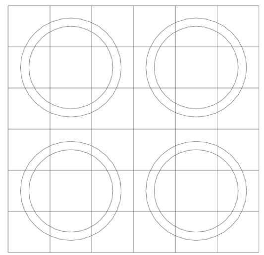
Fig. 9.2.8 Computational grid structure in a NEWT model.
Every unit begins with a header consisting of the keyword unit followed by a unique integer label (unit_id) that serves to identify the unit:
unit unit_id
The header is followed by a complete unit description consisting of the three components described above; each of these components of the unit specification is described in the following subsections. In every NEWT model, one unit must be defined as the global unit. This unit defines the global coordinate system for the entire problem, and all other units (if any) must fit within the global unit. Specification of the global unit is accomplished simply with the format:
global unit unit_id
The global unit may occur anywhere in the list of units. If only one unit is defined in an input, it must be identified as the global unit.
As indicated earlier, the geometry block consists of a list of one or more units. Each unit is terminated by the beginning of another unit or by the end of the geometry block. Conceptually, a geometry block will have the following structure:
read geom
global unit 1
(unit specifications)
unit 2
(unit specifications)
unit 3
(unit specifications)
…
unit 10
(unit specifications)
end geom
The unit numbers are arbitrary and can occur in any order, although they must be unique; they serve simply as labels.
The remainder of this section describes the various components of units.
9.2.4.6.1. Bodies
Every unit contains a set of body specifications in terms of (1) basic shapes that are placed directly within a unit; (2) one or more arrays, each of which is defined elsewhere and placed within a unit with an array placement operator; and (3) holes. Units must contain at least one shape specification, which is used to define the spatial boundaries of the unit. Additional shape specifications may be used as needed. Holes and/or array placements are optional; there is no theoretical limit on the number of each that may be used within a unit.
9.2.4.6.1.1. Shapes
Shapes are simple predefined bodies. NEWT currently supports six shapes:
cylinder,
cuboid,
hexprism,
rhexprism (rotated hexprism),
wedge, and
polygon.
The names of these shapes are generally associated with 3-D bodies but are used in NEWT to be consistent with KENO-VI nomenclature. In NEWT, a cylinder is equivalent to a circle, a cuboid is equivalent to a rectangle, a hexprism is equivalent to a hexagon, and a wedge is equivalent to a triangle.
Because the SGGP is combinatorial in nature, intersection and overlap of shapes is permitted. For this reason, no specific mixture is associated with each shape. Combinatorial logic allows a fraction of a shape to be filled with one mixture, while the remainder or another fraction thereof may be assigned a different mixture. This is discussed further in the section Media Specifications in the description of media assignment (Sect. 9.2.4.6.2).
Each shape is specified by name, an associated body identification (body_id) number, and dimensioning data. The body_id number is arbitrary but must be unique within each unit. Specific formats for each shape are provided below.
9.2.4.6.1.2. Cylinder
Cylinder
The cylinder specification has the following format:
cylinder body_id radius [modifier_list]
where radius is the radius of the circle. The circle will be centered at (0,0). The modifier list is an optional set of operations that may be performed on each shape. One of the modifiers allowed is the origin modifier, which lets one translate the origin of a shape to a different location. Modifier commands are described later in this section.
9.2.4.6.1.3. Cuboid
The cuboid specification has the following format:
cuboid body_id xmax, xmin, ymax, ymin [modifier_list]
where (xmin, ymin) and (xmax, ymax) represent the lower-left and upper-right vertices of a rectangle on a Cartesian coordinate system. Note that the cuboid is explicitly placed by its coordinates; no translation is required (or allowed).
9.2.4.6.1.4. Hexprism and rhexprism
Both hexprisms are specified in a manner identical to that of a cylinder:
hexprism body_id  radius  [modifier_list]
rhexprism  body_id  radius  [modifier_list]
where radius is the inner/minor radius of the hexagon. A standard hexagon (hexprism) is oriented with vertices at the top and bottom, as illustrated in Fig. 9.2.9. A rotated hexagon (rhexprism) is oriented with vertices on the left and right sides, as illustrated in Fig. 9.2.10. Both types of hexprisms, like cylinders, are by default placed with their origins at (0,0). However, like cylinders, they can also be translated in space via the origin translation command.
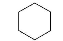
Fig. 9.2.9 Orientation of a standard hexprism.
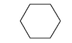
Fig. 9.2.10 Orientation of a rotated hexprism.
9.2.4.6.1.5. Wedge
A wedge, or triangle, specification has the following format:
wedge body_id xbase xpt ypt [modifier_list]
where the vertices of the shape are defined as (0,0), (xbase,0), and (xpt,ypt). Thus, one side always lies on the x-axis. The modifiers origin and rotate may be used to position and orient the triangle in the problem domain. Fig. 9.2.11 illustrates placement of a wedge using these parameters.
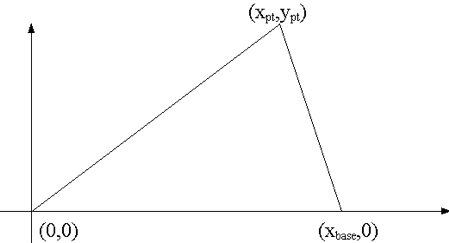
Fig. 9.2.11 Initial positioning of the wedge body.
9.2.4.6.1.6. Polygon
The polygon specification has the following format:
polygon body_id x0, y0, x1, y1, ..., xN, yN, x0, y0
where (xi, yi) are the polygon vertices (the first and last pair in this list refer to the same vertex). Note that the polygon is explicitly placed by its coordinates; no translation is required (or allowed).
9.2.4.6.1.7. Example of shape specifications
Use of shapes within a unit can be illustrated with a simple example. Consider a unit, arbitrarily labeled with unit_id=10, containing a cuboid and two cylinders. Each shape is given a unique (but arbitrary) body_id.
unit 10
cuboid   11   3.0   -5.0   1.0   -2.0
cylinder 12   0.8
cylinder 13   0.6
The cuboid is explicitly placed by its coordinates; the two cylinders will by default be placed at (0,0). Use of the origin command to relocate cylinders is introduced below. Fig. 9.2.12 illustrates the body placement that occurs for the given example.
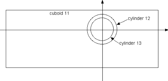
Fig. 9.2.12 Body placement for two cylinders and a cuboid.
9.2.4.6.1.8. Shape modifier commands
Modifier commands are provided as a means to perform specific functions relative to the input shape. The five available modifier commands and the shapes to which they may be applied are listed here:
origin - translation of center bodies (cylinders, hexprisms, rhexprisms);
rotate - rotation of bodies with respect to the transverse axis (all);
chord - removal of a portion of a body with x-plane and y-plane cuts (cylinders, hexprisms, rhexprisms);
com - addition of a comment to a specific shape (all);
sides - number of sides used to approximate a circle (cylinder, default is 12).
The format for each of these commands follows.
9.2.4.6.1.9. ORIGIN
The origin modifier is used to translate the origin of a cylinder or hexprism from the default origin of (0,0) to some other location. It has the format
origin x=xnew y=ynew
where (xnew, ynew) is the new center of the shape. The modifier origin may not be applied to cuboids, as the location of a cuboid is explicitly set by its shape specification. If not specified, each ordinate is set to zero, such that
origin x=5
is equivalent to
origin x=5 y=0 .
For example, consider a cuboid whose lower-left and upper-right corners are located at (0,0) and (1,1), respectively. If one places a cylinder with radius 0.3 in the center of this box [i.e., centered at (0.5, 0.5)], this would be specified as follows:
unit 1
cuboid 10 1.0 0.0 1.0 0.0
cylinder 20 0.3 origin x=0.5 y=0.5
This configuration is illustrated in Fig. 9.2.13.
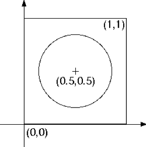
Fig. 9.2.13 Relocation (translation) of a cylinder using origin.
9.2.4.6.1.10. Rotate
The rotate body modifier is used to rotate a body around its geometric center. It can be applied to any body type, but rotation of a cylinder has no real meaning. The format of the rotate modifier is as follows:
rotate a1=A
where A is the angle of rotation, in degrees, in a counterclockwise direction. All bodies lie in the (x,y) plane, with rotation around the z-axis, but with respect to the centroid of the body. Rotation always occurs before translation (via origin), irrespective of the order of rotate and origin commands in the modifier list for a body. KENO-VI allows rotation about the x and y axes as well, through a2= and a3=; however, only rotation about the z axis is permitted in NEWT.
As an example, consider a 1 by 1 cm cuboid centered at (0,0), place a smaller 0.5 by 0.5 cm cuboid inside it, and rotate it 30 degrees clockwise.
unit 1
cuboid 10 0.5 -0.5  0.5 -0.5
cuboid 10 0.25 -0.25  0.25 -0.25 rotate a1=-30
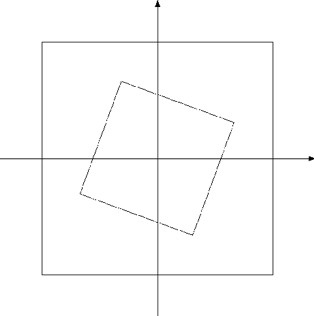
Fig. 9.2.14 Rotation of a cuboid.
Fig. 9.2.14 illustrates the configuration generated using this specification. Note that clockwise rotation was performed by specifying a negative angle. In this case, the centroid of the inner cuboid coincides with (0,0); however, the same geometric rotation would have occurred if the bodies had not been centered at (0,0).
9.2.4.6.1.11. Chord
The chord modifier is used to remove a portion of a body. It provides for horizontal and/or vertical cuts on a body, with the portion of the body on a specified side of that body discarded. Chords may be applied to cylinders or hexprisms but may not be applied to cuboids. (Such “cuts” may be explicitly defined in the body definition.) The format of the specification combines the selection of the plane (horizontal or vertical cut), location of the plane, and the portion of the body to be retained, all in one terse modifier.
The four possible chord specifications for a body are as follows:
chord +x=xplane
chord +y=yplane
chord -x=xplane
chord -y=yplane
where xplane and yplane are the ordinates on the x and y axes, respectively. The sign on x and y indicates the portion of the body to be retained after the cut. A plus (+) sign indicates that the portion of the body in the positive (increasing x or y) direction should be kept, and a minus (-) sign indicates that the portion of the body in the negative direction of the cut plane (decreasing x or y) direction is retained. Chords are applied after any translation (origin) or rotation (rotate) modifier operations. Multiple chords may be specified for a single body to obtain multiple cuts. The keyword chord must precede each specification.
The use of chords is best illustrated by example. Fig. 9.2.15 through Fig. 9.2.18 show unit body descriptions with various chord specifications.
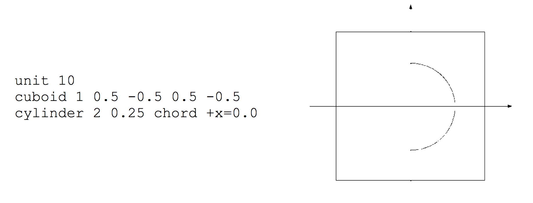
Fig. 9.2.15 Example of chord +x behavior.
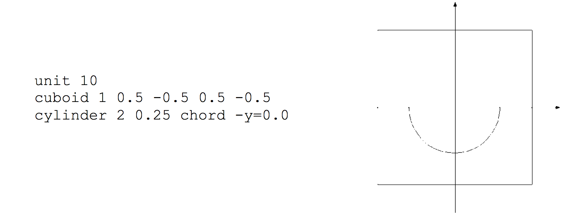
Fig. 9.2.16 Example of chord -y behavior.
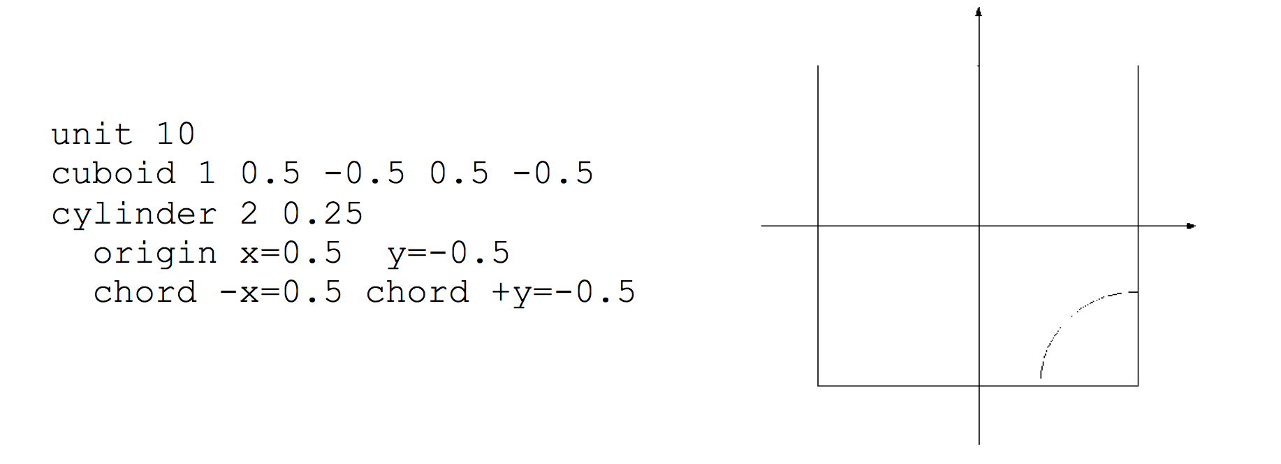
Fig. 9.2.17 Use of two chords to create a quarter-cylinder body.
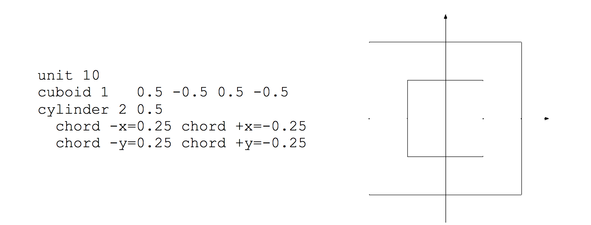
Fig. 9.2.18 Use of four chords on a cylinder to create a square body.
In Fig. 9.2.15, a chord is placed at x=0 and the positive portion relative to the chord (x >0) is retained because +x mode is specified. Since the cylinder is centered at (0, 0), this chord cuts the cylinder in half and retains the right half of the cylinder. The unit in Fig. 9.2.16 uses the same cylinder but with a chord cutting at the plane located at y=0. The bottom half (y < 0) is kept because -y is specified.
Fig. 9.2.17 is somewhat more complicated but represents perhaps the most common use of chords in lattice models. In this case, it is desired to create a one-quarter cylinder located in the bottom right quadrant of a cuboid. A 1 by 1 cm square cuboid is centered at (0, 0), and a cylinder is placed at (0.5, -0.5), which is the lower right-hand corner of the cuboid. Since we are interested only in the portion of the cylinder within the cuboid, we choose to keep the top (+x) and left (-y) portions of the cylinder. This requires two separate chord modifiers. (Each chord specifies only one cutting plane.) Additionally, because the cylinder was relocated to a new origin, the chords are specified such that the cuts go through the new origin.
Note that there is no requirement that a chord cut through the origin of a body. Fig. 9.2.18 illustrates the use of four chords to set four cutting planes. A 0.5 cm cylinder is specified centered within the unit cuboid. All four of the four permitted cutting planes are specified. We have effectively created a cuboid by retaining the portion of the cylinder above (+y) the xz plane located at y= -0.25, below (-y) the plane at y=+0.25, to the right (+x) of the yz plane at x= -0.25, and to the left (-x) of the plane located at x=+0.25. There is, of course, a much more direct means to create a cuboid-this example is provided only for illustrative purposes.
For guidance on how to cut a cylinder at an oblique angle, refer to Sect. 9.2.4.6.1.14.
9.2.4.6.1.12. Com
The com modifier is a means to label specific bodies. It is provided primarily for consistency with KENO-VI. At this time, NEWT simply reads and then ignores com data. It can, however, be used as a means to help annotate an input listing. The format for the com modifier is as follows:
com="comment string"
where “comment string” is any text description of up to 132 characters, delimited by single (‘) or double quotes (“). For example, the input description of Fig. 9.2.18 is shown here with comments added via com modifiers.
unit 10
cuboid 1   0.5 -0.5 0.5 -0.5 com="unit cuboid centered at (0,0)"
cylinder 2 0.5 com="cylinder with four chords"
  chord -x=0.25 chord +x=-0.25
  chord -y=0.25 chord +y=-0.25
9.2.4.6.1.13. Sides
The sides modifier applies only to cylinders and is unique to NEWT (i.e., it is not used in KENO-VI). Because NEWT’s solution grid is based on arbitrary polygons, all cells must be straight sided. Hence, the curved surfaces of a cylinder are approximated as an N-sided regular polygon. By default, N=12. The sides operator allows the user to override the default. The format is very simple:
sides=N
where N is the number of sides desired for the full cylinder. In general, a 12-sided polygon provides an adequate approximation of a cylinder. Use of additional sides will create a cylinder that has a smoother appearance and increase the computational effort required to solve the cells associated with the cylinder.
Fig. 9.2.19 shows a model built with three nested cylinders inside a unit cuboid. Cylinder 10 is the innermost cylinder, with no sides modifier; hence, it uses the default 12-sided approximation. The second cylinder is specified with sides=16; the refinement in this approximation is seen in the figure. Finally, cylinder 30 is specified with 40 sides-this is visually a very close approximation to a cylinder.
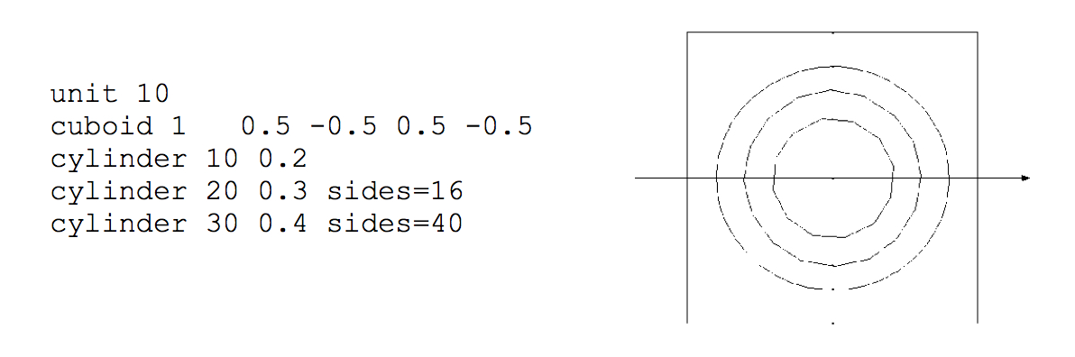
Fig. 9.2.19 Use of the sides modifier for cylinders.
9.2.4.6.1.14. Holes
The next level of complexity within a unit is provided through the use of a hole specification. The hole specification is simply a means by which one unit may be placed within another unit. In some instances, a well-defined set of structures, assembled as a unit, needs to be placed within a larger unit. NEWT provides two methods to do this-holes and arrays. Arrays are used to place a unit (or a number of similar units) in a regular repeating pattern within an enclosing unit. A hole, on the other hand, is a means to place a single unit. This is often used when units being placed do not have a regular repeating pattern.
The format for a hole specification within a unit is as follows:
hole unit_id [modifier_list]
where unit_id is the identification number for the unit that is being placed within the current unit. (A unit cannot be placed within itself.) Unlike the shapes described earlier, holes do not have a distinct identification number of their own-they are simply a mechanism to place a unit defined elsewhere.
By default, the hole operator places the origin of the new unit at the origin (0,0) of the current unit. The origin modifier may also be used with a hole specification to position the placed unit at a location other than (0,0) of the current unit. However, placement of the body is always relative to the origin of the original unit, which can be defined in a number of different ways.
Holes are also associated with a particular shape. Hole specifications must immediately follow the shape into which they are being placed. Holes redefine the boundaries of a shape by figuratively cutting holes in that shape into which units are placed. When mixtures are defined for a given shape (through media specifications, described below), the mixture is placed throughout the region, except in the space excluded by the hole placements.
The rotate modifier can also be applied to a hole, as can the com modifier. However, chord specifications cannot be used to remove a portion of a hole. To construct a cylinder that is cut at an oblique angle, users should construct a cylinder that is cut by a chord and then use the hole operator combined with the origin and rotate modifiers to place and rotate the unit to the desired position and orientation. This can be particularly useful in hexagonal or triangular geometries.
As an example, consider a unit, unit_id=1, consisting of two concentric cylinders, and a second unit, consisting of two concentric cuboids. Descriptions for these two units are given below. Note that these are incomplete unit specifications; other components of the unit specification have not yet been introduced. However, for the purposes of this example, incomplete unit specification will suffice.
unit 1
cylinder  12   0.8
cylinder  13   0.6

unit 2
cuboid 12 0.8 -0.8 0.8 -0.8
cuboid 13 0.6 -0.6 0.6 -0.6
Now suppose that we wished to place two of the unit 1 cells and one of the unit 2 cells inside unit 3, with unit 2 rotated by 45\(^{\circ}\). We can define a cuboid as unit 3 and place the units 1 and 2 inside the cuboid using hole specifications:
unit 3
cuboid 10 4.5 0.0 4.5 0.0
hole 1 origin x=1.3 y=1.3
hole 1 origin x=1.3 y=3.3
hole 2 origin x=3.1 y=2.3 rotate a1=45
In this example, a square cuboid is defined such that its lower-left corner is situated at (0,0). Three hole operations are used: the first to place unit 1 at (1.3, 1.3), the second to place another instance of unit 1 2 cm above the first, at (1.3, 3.3). Lastly, unit 2 is placed inside unit 3 at (3.1, 2.3) and then rotated 45\(^{\circ}\). Fig. 9.2.20 illustrates how such a unit would appear.
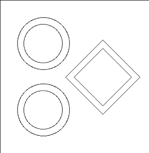
Fig. 9.2.20 Unit placement within a unit using holes.
9.2.4.6.1.15. Array placement
As indicated in the previous section, arrays are a method for arranging one or more units within another unit. Arrays specifications are typically used when units are placed in a repeating pattern. While the hole specification is used to place different units within a given unit, the array placement specification is used to place an array within a unit.
All arrays are specified (declaration of size, type, and fill) in the array data block, as described in Sect. 9.2.4.9. The array placement operator is used to locate an array within a unit. The format for the array placement operator is as follows:
array arrayid body_id place i j xij yij
where arrayid is the identification number assigned to the array in the array data block and body_id is the identification number of the shape into which the array is placed. The remainder of the array placement operator is used to fix the position of the array within the body, identified by body_id. A general discussion of this concept follows, after which the actual placement of the array is described.
Arrays are defined by two dimensioning parameters-the number of rows and the number of columns. Each element of an array is filled by a unit; each unit has its own local coordinate system. In other words, one unit may have the origin (0,0) in its local coordinate system defined as the lower-left corner while another unit may have its origin defined at its geometric center. The array itself has no coordinate system; it is simply a list of relative positions of units, defined by their row/column position. The place directive of the array placement operator is used to locate the array within the body into which it is being placed.
In the place directive, i represents the column (counting from left to right) and j represents the row (counting from bottom to top) of a specific element of the array. The coordinate system of that specific unit is used to set the position of the entire array. The coordinates xij and yij represent the location in the current unit where the array is to be placed. Placement occurs by situating the origin of the unit in column i, row j at coordinate (x:sub:ij,yij). Placement of arrays within a unit is best understood through examples. Consider three (partial) unit specifications, as defined and illustrated in Fig. 9.2.21.
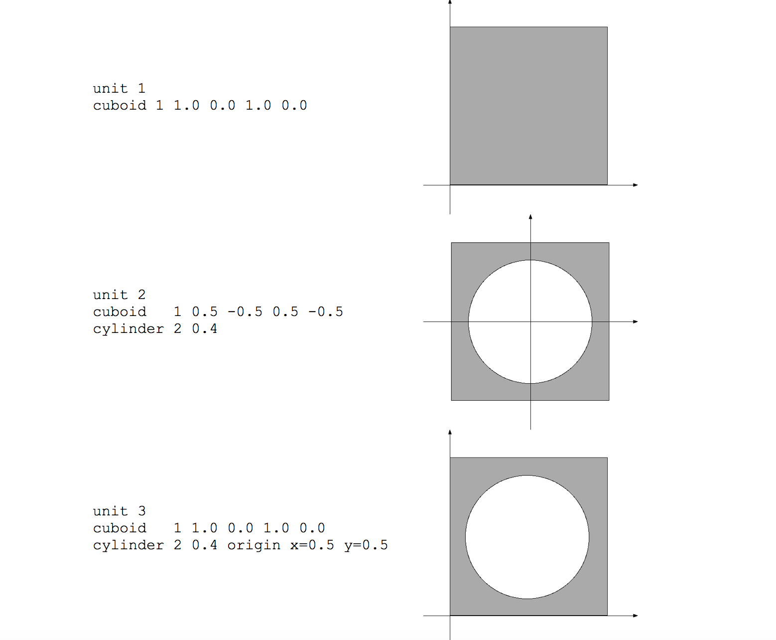
Fig. 9.2.21 Example of units to be placed in an array.
Unit 1 is a simple 1 by 1 cm cuboid with its origin located at its bottom-left corner; unit 2 is a similar-sized cuboid but with its origin located at its geometric center and with a cylinder centered in it; and unit 3 is identical to unit 1 but with a cylinder centered in it. Units 2 and 3 are identical in structure but use a different local coordinate system.
Now assume an array has been defined in the array data block and assigned arrayid=50. The relative positions of the units are shown in Fig. 9.2.22; unit 3 is located in row 1, column 1.
We desire to place this array within a unit 4, a 2 by 2 cm cuboid with its lower-left corner located at (0,0). Because there are four different array positions, this array has four possible placements:
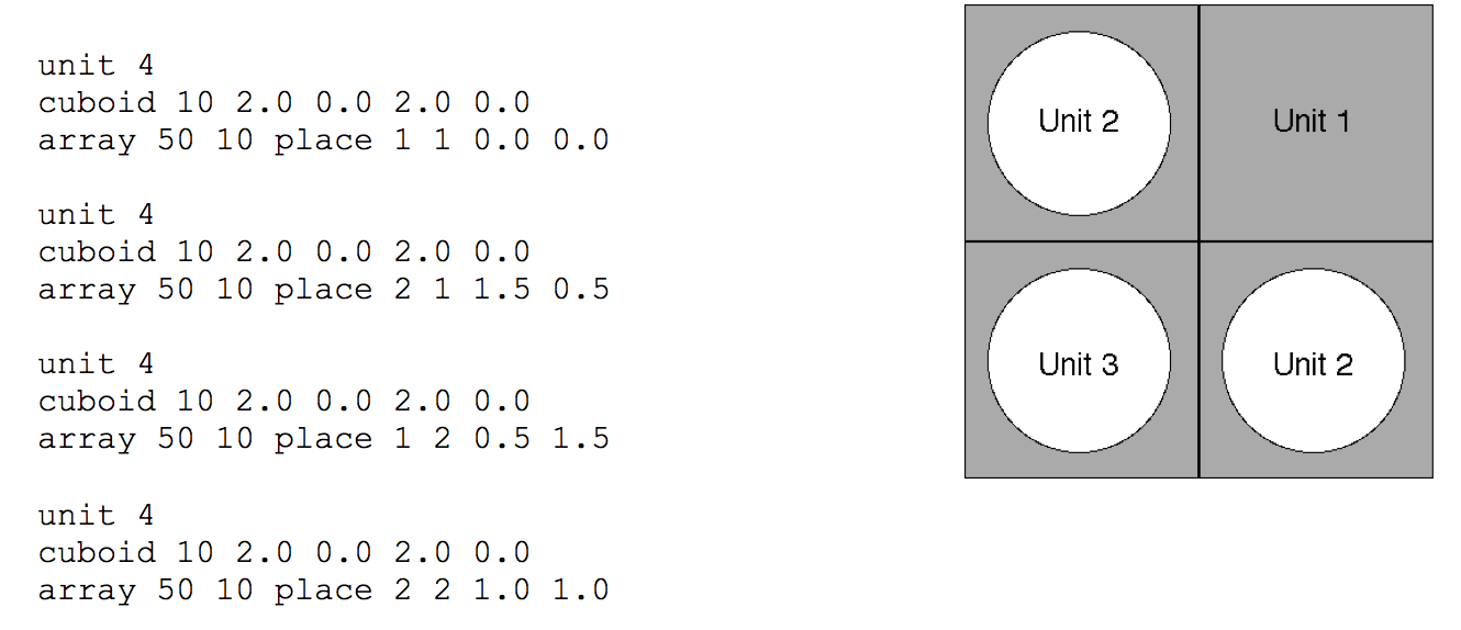
Fig. 9.2.22 Layout of units in array 50.
For the first example, the unit located in row 1, column 1 (i.e., unit 3) is placed such that its origin (its lower-left corner) is located at (0,0), which is the origin of unit 4. For the second example, the unit located in column 2, row 1, is placed such that its local origin, which is in the center of the unit, is located at x=1.5, y=0.5 in the coordinate system of unit 4.
9.2.4.6.2. Media specifications
A unit is only partially specified by its constituent bodies. At this point, no composition has been associated with the various regions of the problem nor has the outer boundary of the unit been defined. This section provides information on the use of media specifications to define the contents of each shape that has been defined.
Each shape statement defines a basic shape, with optional modifiers, which represents a spatial region within the unit. Assignment of compositions to regions is performed via media specifications.
As discussed earlier in the introduction to shapes, input processing in the SGGP is combinatorial. This permits intersection of shapes, and different compositions (or media) may be assigned to different portions of intersecting bodies.
The format of a media specification is as follows:
media materialid bias_placeholder reg_def_vector
where materialid is the composition number being placed in this entry, bias_placeholder is a simple placeholder that is required but not used, and reg_def_vector is the region definition vector used to define the shape or shapes to which the mixture is assigned.
The bias_placeholder is used to be as consistent as possible with KENO-VI input. KENO-VI allows the user to assign biases within the media assignments to improve the Monte Carlo solution performance. Biases have no meaning in NEWT, so the field has no meaning. In KENO-VI, if no special biasing is desired, a value of 1 is assigned. If it is desired to move models between NEWT and KENO-VI format, a placeholder value of 1 is recommended. However, the value itself has no meaning within NEWT; it is simply read and ignored. (This may change in a future release.)
The region definition vector is used to describe the location of the composition within the current unit. This is done by providing a list of shapes for which the media is either “inside” or “outside.” The sense of the media with respect to a shape is specified by listing the shape number with a negative sign if “outside” and with a positive (or no) sign when the media is placed “inside” the shape.
Consider a simple cylinder inside a cuboid. Assume composition 1 is to be placed inside the cylinder and composition 2 outside the cylinder but inside the cuboid. The shape and media specifications could have the following format:
unit 1
cylinder 10 0.5
cuboid 20 1.0 -1.0 1.0 -1.0
media 1 1 10
media 2 1 20 -10
In the above example, the first media record places mixture 1 inside all of shape 10 (the cylinder). The second media entry places mixture 2 in all regions that are outside shape 10 but inside shape 20. Note also that a bias placeholder value of 1 is used in each media statement.
It is necessary to specify media for all regions of the unit. If any regions remain unassigned, NEWT will stop with an error message. If the second record had been omitted, regions outside the cylinder would be unspecified and the code would stop. Note also that if the second media statement had read only
media 2 1 20
then composition 2 would have been placed inside all of cuboid 20, including inside the cylinder 10. The fact that the contents of 10 have already been specified is ignored. The above statement directs the code to put mixture 2 everywhere inside the boundaries of the cuboid.
Each region definition vector combines all specifications with a logical
AND. In other words, the second media record in “media 2 1 20” places
composition 2 in all regions that are simultaneously outside shape 10
and inside shape 20. Separate media specifications are required to
place a composition in two independent shapes. The following represents
a cuboid with two nonintersecting cylinders.
unit 1
cylinder 10 0.4 origin x=0.5
cylinder 20 0.4 origin x=1.5
cuboid 30 2.0 0.0 1.0 -1.0
media 1 1 10
media 1 1 20
media 2 1 30 -10 -20
A media statement is necessary to place composition 1 inside shape 10; a similar statement is necessary to place composition 1 inside shape 20. Finally, all space inside cuboid 30 but outside both 10 and 20 is filled with composition 2. If one attempted to fill both 10 and 20 with composition 1 in a single media record, for example,
media 1 1 10 20
then an error would occur. The code would attempt to place composition 1 in all space that is simultaneously within shape 10 and within shape 20-and no such space exists.
A more common example is the configuration of a fuel pin (composition 1), gas gap (composition 2), clad (composition 3), and moderator (composition 4) in a lattice. Consider a pin in a hexagonal lattice:
unit 1
cylinder 10 0.4
cylinder 20 0.41
cylinder 30 0.5
hexprism 40 0.8
media 1 1 10
media 2 1 20 -10
media 3 1 30 -20
media 4 1 40 -30
In this example, for the hexagonal moderator region outside the clad, it is sufficient to specify that mixture 4 is inside 40 and outside 30. Although it is true that the moderator is also outside shapes 10 and 20, it is not necessary to specify this. Logically, since 10 and 20 are inside 30, then everything outside 30 must be outside 10 and outside 20. The use of a hexprism in this example is irrelevant. If the outer body had been a cuboid, the result would have been the same.
As a final example, consider a unit with intersecting bodies. It becomes possible to assign a unique composition to each intersection of shapes (Fig. 9.2.23).
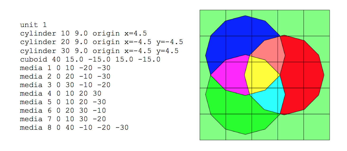
Fig. 9.2.23 Media assignments in overlapping regions.
In this model, cylinder 10 is on the right, 20 is the lower left, and 30 is the upper left. Media 1, placed inside cylinder 10 but outside 20 and 30, is represented by the partially filled right-hand side of the right cylinder. The central region of the unit is filled with composition 4 and represents all areas that are simultaneously within shapes 10, 20, and 30. The outermost region is everything that is inside 40, but outside 10, 20, and 30.
Media statements apply only to shapes, and only to those shapes within the unit. Holes and array specifications are used to define placement of one or more units in which media have already been specified in the corresponding unit definitions. Like shape statements, media statements may occur in any order. However, if one region is erroneously assigned two different compositions in two different media statements, the code will allow this and will proceed with the calculation. The last specification for a shape will always take precedence. Thus, it is important that newly developed models be visually inspected using mixture plots (files named “.newtmatl.ps”) created using *drawit=yes in the parameter block.
9.2.4.6.2.1. Unit boundary
The final section of a unit description is the boundary specification. This input record serves two purposes: to specify the shape that defines the outer bounds of the unit, and hence the shape of the unit, and (optionally) to specify the underlying grid associated with the unit. The format of the boundary specification is as follows:
boundary body_id [x-discretization y-discretization]
where body_id is the identification number for the body that is to serve as the unit boundary. The x-discretization and y-discretization terms are integers (\(\geq\) 2) that specify the number of rectangular cells to be placed in the unit in the x-direction and y-direction, respectively. A grid specification is required for the global unit but is optional for other units. If a grid is specified for a grid other than the global unit, that grid replaces the base grid. (An exception to this principle is discussed later.)
In general, grid refinement should be such that cell sizes are on the order of or smaller than a mean free path for a neutron. Grid spacing can be easily varied in order to converge on the parameter of interest. Global factors, such as a system eigenvalue, can tolerate a relatively coarse grid. However, if fluxes are known to vary rapidly in space, then a more refined grid may be necessary. NEWT does provide the ability to locally refine a grid structure so that detail can be modeled where needed, without having to pay the computational penalty of refining the grid everywhere. NEWT does place one limit on grid refinement: every shape, hole, or array placed within a unit must be intersected by at least one gridline. The grid may be locally defined or part of the global grid, but it must intersect each body at least once. Thus, if small geometric shapes are modeled, a detailed grid structure is generally necessary.
Examples of boundary specifications follow, as parts of partial unit specifications. Media descriptions are omitted for simplicity. Accompanying figures illustrate the grid structure(s) associated with each specification. Fig. 9.2.24 shows a single (global) unit with a 2 by 2 base grid. Cuboid 10 serves as the boundary for the unit. This represents the minimum grid structure that can be specified for a unit. Fig. 9.2.25 shows a more complex configuration in which a unit defined with a 5 by 5 grid is placed in the center of a larger enclosing unit, specified to have a 3 by 3 grid. Note that because the first unit has its own (local) grid, the underlying grid structure is removed in favor of the local grid structure. The grid is applied to the boundary shape of the unit, which is cuboid 10.
Fig. 9.2.26 shows a similar structure; however, the cuboid was removed from unit 1 and the outer hexprism was defined as the unit boundary. Note that the grid structure applied to the nonrectangular body is the same as the one that would be assigned for a cuboid with the same minima and maxima in x and y directions. Fig. 9.2.27 illustrates the grid structure that would be applied to the same model as was used in the previous figure but with CMFD acceleration enabled. Because CMFD is normally applied to a coarse mesh defined by the base global grid (unless xycmfd=0), the global grid is always retained when CMFD acceleration is used. Finally, Fig. 9.2.28 illustrates the use of a base grid only. In this case, no grid structure is assigned for unit 1; the bodies are inlaid but are adapted to the base global grid structure.
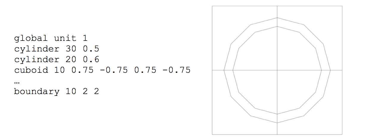
Fig. 9.2.24 Unit with 2 by 2 grid in a simple pin-cell model.
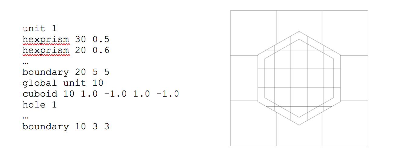
Fig. 9.2.25 Unit with 5 by 5 grid inset into unit with 3 by 3 grid.
Fig. 9.2.26 Effect of boundary grid specification on noncuboidal unit placed as a hole within a larger unit.
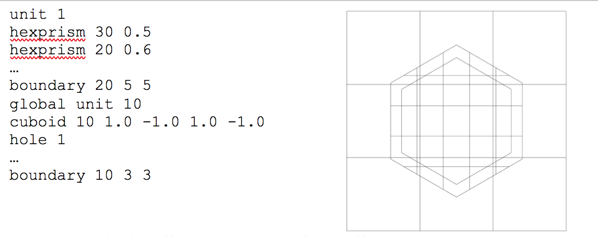
Fig. 9.2.27 Effect of coarse-mesh finite-difference acceleration on grid structure.
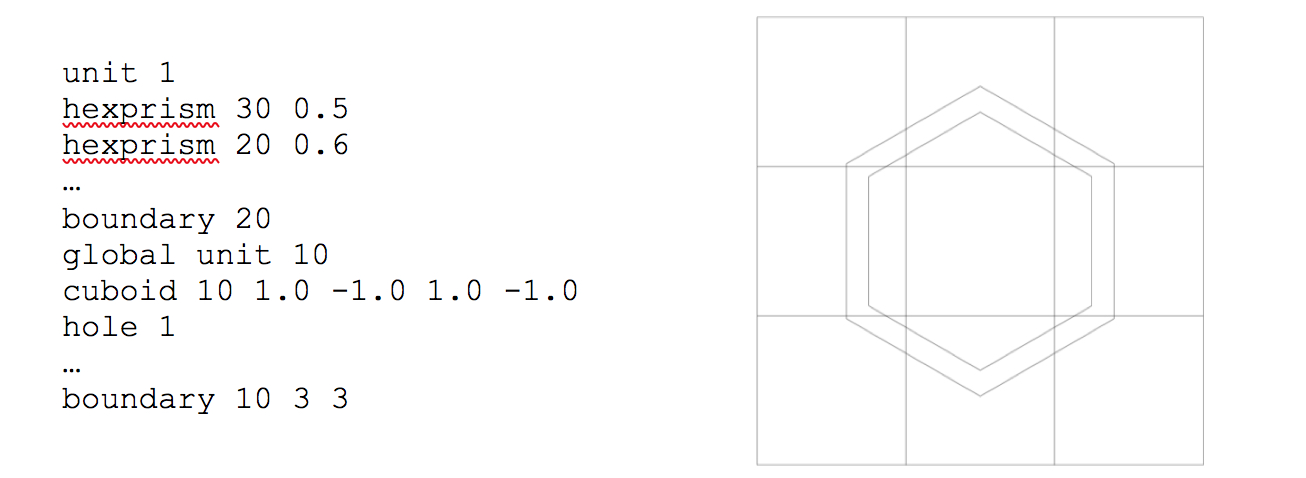
Fig. 9.2.28 Use of base grid without localized grid specification.
The following section provides examples of complete geometry specifications for various models, including bodies, media, and boundary specifications. Each will include one or more uses or boundary specifications for units.
9.2.4.6.3. Geometry block examples
The following three subsections present geometry block examples to show how various models may be assembled. Each listing is described briefly and is followed by a figure showing the NEWT grid structure generated for each set of geometry instructions.
9.2.4.6.3.1. Simple pin cell
The following geometry block (Fig. 9.2.29) shows the specifications necessary to define a single pin-cell. The model is reduced to a \(1/4\) cell to take advantage of symmetry. Mixture 1 is fuel, mixture 2 is fill gas, mixture 3 is clad, and mixture 4 is moderator. Features of this model include the use of chords to obtain \(1/4\) cylinders and the specification of 20 sides for each cylinder (five sides for a \(1/4\) cylinder).
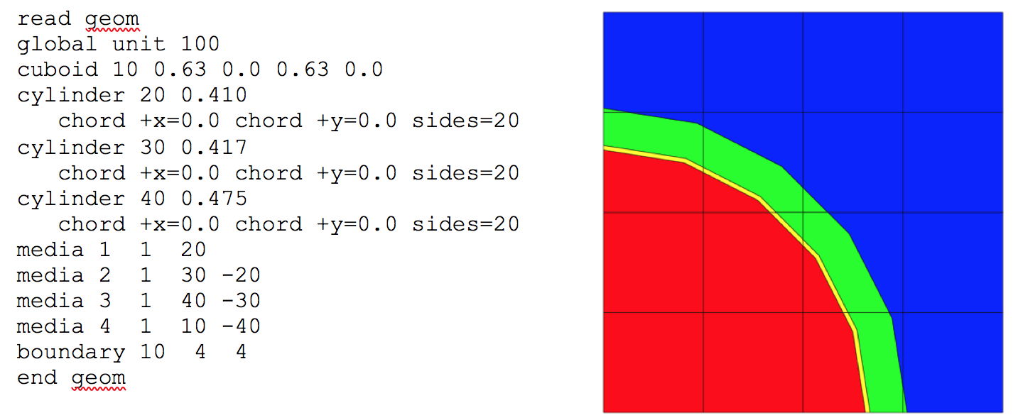
Fig. 9.2.29 Geometry model for infinite-lattice pin cell with fuel, gap, clad, and moderator.
9.2.4.6.3.2. Hexagonal assembly
The geometry block below (Fig. 9.2.30) is used to describe a hexagonal fuel assembly within a hexagonal shroud. Each cylinder is placed individually, followed by a series of media statements that fill each cylinder. The hexagonal moderator area is surrounded by a hexagonal shroud of cladding material. Note that NEWT allows only cuboid and hexprisms as outer boundaries for the global unit. This model could also have been assembled with a unit definition for a set of cylinders, which could then be placed in the global unit using holes or by defining a single pin cell and placing it using an array.
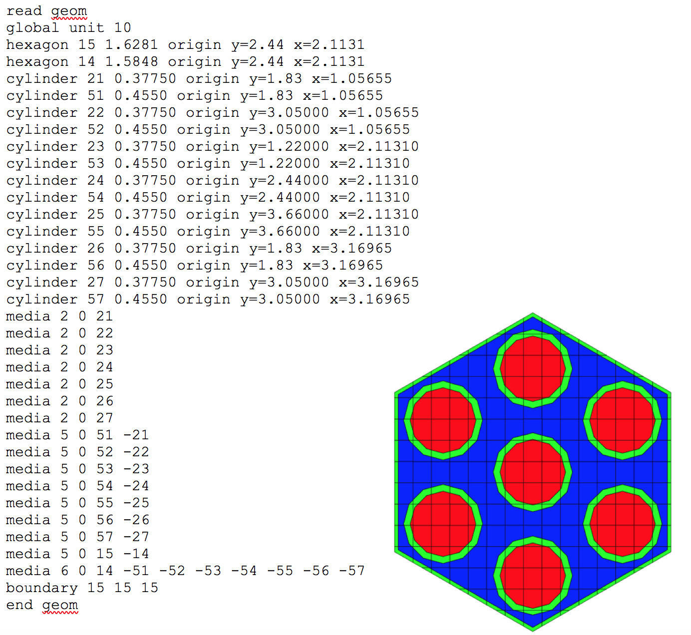
Fig. 9.2.30 Geometry model of hexagonal fuel assembly.
9.2.4.6.3.3. Advanced CANDU reactor ACR-700 assembly
This example of a geometry block (Fig. 9.2.31) is included to illustrate the complexity of design that is possible through the use of simple bodies, units, and holes. The ACR-700 design cannot be modeled using an array because pins are not placed in a repeating lattice pattern. Features of this example include use of holes; use of noncuboidal units placed in holes; and localized pin-cell grid refinement by (1) decreased mesh size in fuel elements (three outer rings) and (2) increased radial discretization (central pin).
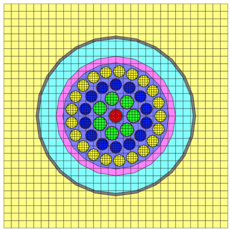
Fig. 9.2.31 ACR-700 fuel assembly model.
read geom

'central pin
unit 1
cylinder 101 0.200
cylinder 102 0.400
cylinder 103 0.529
cylinder 104 0.629
cylinder 151 0.675
media 11 104
media 11 1 151 -104
boundary 151 2 2

'first ring pin
unit 2
cylinder   201  0.629
cylinder   251  0.675
media      2  1  201
media     21  1  251 -201
boundary 251 5 5

'second ring pin
unit 3
cylinder   301  0.533
cylinder   351  0.575
media      3  1  301
media     31  1  351 -301
boundary 351 5 5

'third ring pin
unit 4
cylinder   401  0.533
cylinder   451  0.575
media     4   1  401
media     41  1  451 -401
boundary  451 5 5

global unit 10
cuboid   100  11 -11 11 -11
cylinder   500  5.1689 sides=20

hole 1
hole 2  origin x=-1.56318 y= 0.75279
hole 2  origin x=-0.38607 y= 1.69150
hole 2  origin x= 1.08176 y= 1.35648
hole 2  origin x= 1.73500
hole 2  origin x= 1.08176 y=-1.35648
hole 2  origin x=-0.38607 y=-1.69150
hole 2  origin x=-1.56318 y=-0.75279
hole 3 origin x=-2.99790 y= 0.68425
hole 3 origin x=-2.40413 y= 1.91723
hole 3 origin x=-1.33419 y= 2.77048
hole 3 origin            y= 3.07500
hole 3 origin x= 1.33419 y= 2.77048
hole 3 origin x= 2.40413 y= 1.91723
hole 3 origin x= 2.99790 y= 0.68425
hole 3 origin x= 2.99790 y=-0.68425
hole 3 origin x= 2.40413 y=-1.91723
hole 3 origin x= 1.33419 y=-2.77048
hole 3 origin x= 0.00000 y=-3.07500
hole 3 origin x=-1.33419 y=-2.77048
hole 3 origin x=-2.40413 y=-1.91723
hole 3 origin x=-2.99790 y=-0.68425
hole 4 origin x=-4.33602 y= 0.65355
hole 4 origin x=-3.95075 y= 1.90258
hole 4 origin x=-3.21443 y= 2.98256
hole 4 origin x=-2.19250 y= 3.79752
hole 4 origin x=-0.97575 y= 4.27506
hole 4 origin x= 0.32769 y= 4.37274
hole 4 origin x= 1.60202 y= 4.08188
hole 4 origin x= 2.73400 y= 3.42833
hole 4 origin x= 3.62306 y= 2.47016
hole 4 origin x= 4.19019 y= 1.29250
hole 4 origin x= 4.38500
hole 4 origin x= 4.19019 y=-1.29250
hole 4 origin x= 3.62306 y=-2.47016
hole 4 origin x= 2.73400 y=-3.42833
hole 4 origin x= 1.60202 y=-4.08188
hole 4 origin x= 0.32769 y=-4.37274
hole 4 origin x=-0.97575 y=-4.27506
hole 4 origin x=-2.19250 y=-3.79752
hole 4 origin x=-3.21443 y=-2.98256
hole 4 origin x=-3.95075 y=-1.90258

hole 4 origin x=-4.33602 y=-0.65355
cylinder   501  5.8169 sides=20
cylinder   502  7.55   sides=24
cylinder   503  7.8    sides=24
media     13  1  500
media      5  1 501 -500
media      6  1 502 -501
media      7  1 503 -502
media      8  1 100 -503
boundary  100 50 50

end geom
9.2.4.6.4. Summary of geometry specifications
This section is provided as a quick reference for geometry statements. Details and examples of the usage of each geometry specification are provided in previous subsections of this manual. For each definition, the lists of permitted modifiers are listed.
9.2.4.6.4.1. Unit definition statements
[global] unit unit_id
The unit statement is used to initiate the definition of each unit used. unit_id is an integer identification label for the unit and must be unique. One (and only one) global unit is required in each geometry model. Modifiers: none.
cuboid body_id xmax xmin ymax ymin [modifier_list]
The cuboid statement is used to define a rectangular shape. body_id is the integer identification label for the cuboid and must be unique within the unit it is used. The rectangle is defined such that the coordinates (xmin, ymin) and (xmax, ymax) represent the lower-left and upper-right vertices of the cuboid. Modifiers: rotate, com.
cylinder body_id radius [modifier_list]
The cylinder statement defines a circle with integer label body_id and radius radius, placed with its center at the origin (0,0) of the unit. Modifiers: origin, rotate, chord, sides, com.
hexprism body_id radius [modifier_list]
The hexprism statement defines a standard hexagon with integer label body_id and inscribed radius radius, placed with its center at the origin (0,0) of the unit. A standard hexagon has vertices located on north (top) and south (bottom) regions of the shape. Modifiers: origin, rotate, chord, sides, com.
rhexprism body_id radius [modifier_list]
The rhexprism statement defines a rotated hexagon with integer label body_id and inscribed radius radius, placed with its center at the origin (0,0) of the unit. A rotated hexagon has vertices located on east (right) and west (left) regions of the shape. Modifiers: origin, rotate, chord, sides, com.
wedge body_id xbase xpt ypt [modifier_list]
The wedge statement defines a triangle with integer label body_id placed with a vertex at (0,0), a vertex at (xbase,0), and a vertex at (xpt,ypt). Modifiers: origin, rotate, com.
array arrayid body_id place i j xij yij [modifier_list]
The array placement statement specifies the placement of an array with identification number arrayid (defined in the array data block), within shape body_id. If the place statement is used, the array element located in row i (counted from the bottom) and column j (counted from the left) is placed such that its origin is located at spatial coordinate (xij, yij) of the unit in which it is placed. Modifiers: com.
hole unit_id [modifier_list]
The hole statement is used to place a different unit identified by label unit_id within the current unit. The origin of the unit being placed will be located at the origin of the current unit but can be repositioned using the origin modifier. Modifiers: origin, rotate, com.
media materialid bias_placeholder reg_def_vector
The media statement assigns material properties associated with mixture index materialid to a shape region defined within a unit. The bias_placeholder term is not currently used but is retained for consistency with KENO-VI; typically it is assigned a value of 1. reg_def_vector is the region definition vector and assigns the mixture placement relative to shapes within the unit. If the index is positive, the shape region is included in the material assignment; if negative, it is excluded. Modifiers: none.
boundary body_id [x-discretization y-discretization]
The boundary statement is used to define the outer boundary of the unit, corresponding to the outer bounds of the shape body_id within the unit. This shape must exist and must contain all other bodies associated with the unit. The x-discretization and y-discretization terms are integers (\(\geq\) 2) that specify the number of cells to be placed in the unit in the x-direction and y-direction, respectively. A grid specification is required for the global unit but is optional for other units. Modifiers: none.
9.2.4.6.4.2. Geometry modifiers
origin x=xnew y=ynew
Used to relocate the origin of cylinders, hexprisms, rhexprisms, and holes to new co-ordinate (xnew, ynew). The default (if not specified) is to place the origin of the body at (0, 0).
rotate a1=A
Causes a body to be rotated by an angle of A degrees (counterclockwise) around its origin. It can be applied to holes and all basic shapes; the default is 0 degrees.
chord  +/- x=xplane
chord  +/- y=yplane
Chords are used to truncate a shape at the line x=chord (or
y=chord). Multiple chord commands are allowed, but only one line
(either in x- or y-direction) is specified for each. If the negative
keyword -x (or -y) appears, then the part of the shape to the left
of (below) the chord cut is retained. Similarly, if the positive keyword
(-x or -y) is used, then the portion of the shape to the right of or
above the chord is retained. Chords may be applied to cylinders,
hexprisms, and rhexprisms only.
sides=N
For use with the cylinder statement, the sides modifier specifies the number of sides on the regular polygon used to approximate the cylinder. Its default is N = 12. The radius of the polygon is adjusted such that the area of the polygon matches the area of the cylinder it is approximating. The sides modifier is unique to NEWT and is not used by KENO-VI.
9.2.4.7. Boundary conditions
The geometry data block is generally followed by the bounds data block, in which boundary conditions for the sides of the bounding shape in the global array are specified. NEWT supports the use of cuboid, hexprism, and wedge shapes to define outer boundaries. This results in the need to specify up to 6 surface boundaries, on up to 8 spatial orientations. In other words, a cuboid will have boundaries on +x, -x, +y, and -y faces. A regular hexprism will have boundaries on +x and -x faces; it will also have boundaries on the four sloped sides of the hex. In order to identify the sense of sides for specification of boundary conditions, NEWT applies an eight-point compass nomenclature. The four permitted rectangular boundary surfaces are identified as +x, -x, +y, and –y, corresponding to east (E), west (W), north (N), and south (S) faces, as illustrated in Fig. 9.2.32 Sloped (non-rectangular) surfaces are identified as +x+y, +x-y, -x-y, and -x+y, for northeast (NE), southeast (SE), southwest (SW), and northwest (NW) surfaces. No assumptions are made on the slope of the various non-rectangular surfaces; for the bodies available within NEWT, it is not possible to have more than one surface in each octant.

Fig. 9.2.32 Two-dimensional boundary condition surface orientations.
Currently, full specification of boundary conditions is permitted only when the boundary body for the global unit is a cuboid. Only white and vacuum boundary conditions are permitted on non-rectangular surfaces.
Boundary conditions therefore may only be specified for the \(\pm\) x and \(\pm\) y faces of a boundary cuboid. Four boundary conditions are currently supported:
reflective (default),
white,
vacuum, and
periodic.
Albedo boundary conditions are not yet supported but will be available in a future release. Additional information on the meaning of each boundary condition type is provided in the following section.
9.2.4.7.1. Boundary conditions descriptions
Boundary conditions are mathematical approximations used to describe the behavior of neutrons when they cross a problem boundary. Typically, transport methods provide for reflective (or mirror), white, vacuum, or periodic boundary conditions. The following subsections describe and illustrate these four types of boundary conditions.
9.2.4.7.1.1. Reflective boundary condition
For the reflective boundary condition, the incoming angular flux is set equal to the outgoing angular flux in the direction corresponding to mirror or specular reflection. As shown in Fig. 9.2.33, a given quantity of neutrons leaving a boundary (dotted line) in a particular direction will be returned (solid line of same color) to the system with the same quantity but at a mirrored angle to the initial leakage direction.
Note
In the following figures, a dashed arrow indicates neutrons leaving the system while a solid arrow represents those returning to the system. The length of the arrow is proportional to the number of neutrons; therefore, longer arrows represent more neutrons than do shorter arrows.
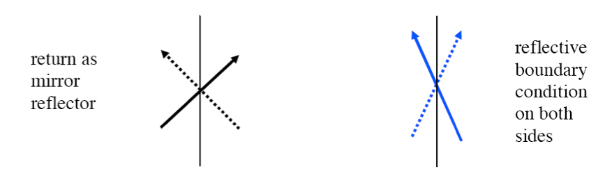
Fig. 9.2.33 Reflective boundary condition.
9.2.4.7.1.2. White boundary condition
For the white boundary condition, the incoming angular fluxes are each set equal to a single value chosen such that the net flow across the boundary is zero. The white boundary provides isotropic return (solid lines) at a boundary (Fig. 9.2.34).
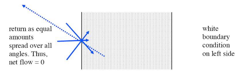
Fig. 9.2.34 White boundary condition.
9.2.4.7.1.3. Vacuum boundary condition
A vacuum boundary condition means that no neutrons will reenter the boundary. Thus, any neutron exiting the system through a boundary with a vacuum boundary condition is permanently lost to the system. This condition is illustrated in Fig. 9.2.35.
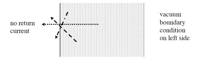
Fig. 9.2.35 Vacuum boundary condition.
9.2.4.7.1.4. Periodic boundary condition
For the periodic boundary condition, the incoming angular flux on a boundary is set equal to the outgoing angular flux on the opposite boundary. Fig. 9.2.36 shows the leakage leaving each boundary (dotted lines) being returned at the same quantity and angle on the opposite boundary (solid line of same color). When the periodic boundary condition is used, it must be applied to both opposing boundaries.
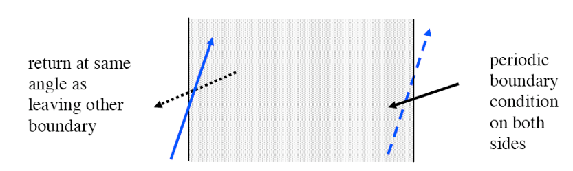
Fig. 9.2.36 Periodic boundary condition.
9.2.4.7.2. Boundary condition specification
The standard format for boundary condition specifications is as follows:
read bounds
-x=west_BC  +x=east_BC  -y=south_BC  +y=north_BC
+x+y=northeast_BC   +x-y=southeast_BC
-x+y=northwest_BC   -x-y=southwest_BC
end bounds
where west_BC, east_BC, south_BC, north_BC, northeast_BC, southeast_BC, northwest_BC, southwest_BC are each one of the eight possible boundary condition options. The name of the boundary condition requires only the number of leading characters required to make the name unique. For this set, the first letter is sufficient; that is, +x=v, +x=vac +x=vacu, and +x=vacuum are all equivalent and specify a vacuum (zero return) boundary condition on the right side of the global cuboid.
In keeping with KENO-VI, multiple shortcuts exist to simplify the specification. For example, a single boundary condition can be assigned to all four sides simultaneously with the all= specifier:
read bounds
all=refl
end bounds
All KENO-VI boundary face keywords that do not reference the z-dimension are allowed and are listed in Table 9.2.1.
Keyword |
Boundary edge |
|---|---|
+x, +xb |
East (right) |
-x, -xb |
West (left) |
+y, +yb |
North (top) |
-y, -yb |
South (bottom) |
all, xyf, yxf |
All boundaries |
+xy, +yx, +fc |
East (right) + north (top) |
-xy, -yx, -fc |
West (left) + south (bottom) |
xfc |
West (left) + east (right) |
yfc |
North (top) + south (bottom) |
+x+y |
Northeast (top right) |
-x+y |
Southeast (bottom right) |
-x-y |
Southwest (bottom left) |
-x+y |
Northwest (top left) |
9.2.4.8. General cross section weighting
NEWT performs cross section weighting by mixture and optionally by homogenization zone (Sect. 9.2.4.10). Weighting is always used in conjunction with an energy collapse. Cross section weighting is performed over a spatial and energy domain; the resulting average (weighted) cross sections will preserve all reaction rates in the collapsed cross section set; that is,
where
\(\sigma_{G}^{i}\) \(\equiv\) average (weighted) cross section in energy group G for nuclide I,
\(N^{i}(r)\) \(\equiv\) number density of nuclide i in region r,
\(W(E, r)\) \(\equiv\) the weighting function within region r,
\(\sigma^{i}(E, r)\) \(\equiv\) the cross section from the input library for nuclide i in region r.
Within NEWT, each collapsing region is the spatial region or regions in which a given mixture is placed. Hence, for most of the cross section types, an average cross section for the mixture associated with the spatial domain r (which may include one or more defined regions occupied by that mixture) is calculated by weighting the original problem-specific cross section data for that mixture using as a weighting function the neutron spectrum calculated within spatial domain r.
In practice, the integration of Eq. (9.2.29) is performed as a simple summation over all cells j within region r:
Because any region r is defined as the sum of all spatial regions containing a given mixture, is constant everywhere within r.
All multigroup cross sections and related data present on the AMPX library are weighted using appropriate weighting functions. For most basic cross sections, the multigroup flux obtained from the transport solution is the appropriate weighting function and \(W_{g, r}\) in Eq. (9.2.30) becomes \(\phi_{g, r}\). However, special cross sections and data need special treatment, as described in the following sections.
9.2.4.8.1. Scattering cross section transfer matrix weighting
In weighting scattering cross sections, the form of the weighting is slightly more complex:
or, in multigroup format,
In general, the scalar flux, \(\phi\)g,r is the appropriate weighting function for scattering cross sections:
This is an approximation for the higher order moments (l > 0) of the scattering cross sections, which should be more properly weighted using the lth moment of the flux instead of the 0th moment (scalar) flux as used in Eq. Eq. (9.2.33). However, because flux moments are generally both positive and negative, NEWT performs higher-order-moment scattering cross section weighting using the positive scalar flux.
9.2.4.8.2. Weighting of the collapsed fission spectrum, \(\chi\)
Weighting is not required for collapsing a fission spectrum vector; the format for a collapsed fission spectrum (\(\chi\)G) is a very straightforward summation of the fission spectra in energy groups g spanning the energy domain of the collapsed energy group G:
9.2.4.8.3. Weighting of the number of neutrons per fission
Accurate weighting of \(v\) in an energy and space domain requires weighting by the fission rate; that is,
Hence, for \(\nu\), Eq. Eq. (9.2.33) has the form
9.2.4.8.4. Weighting of (n,2n), (n,3n), and (n,4n) cross sections
In creating AMPX weighted libraries with NEWT, all data on the original library are collapsed and written to a collapsed working-format library, for each reaction type and for each nuclide. Therefore, each of the (n,*X*n) libraries is collapsed independently using Eq. Eq. (9.2.30) and is written on the weighted library.
However, during NEWT transport calculations, NEWT computes and stores a single effective (n,2n) reaction rate, determined as the weighted sum of the individual reactions:
The (n,2n) reaction rates reported in NEWT output are those computed for the effective cross section. The effective (n,2n) cross section is not saved to the weighted library.
9.2.4.8.5. Calculation and weighting of transport cross sections
Transport cross sections are processed in a different manner from other cross sections. The transport cross section does not represent a purely measurable quantity. Introduced within the P1 (diffusion) approximation to the neutron transport equation, it attempts to preserve a flux gradient in addition to reaction rate information. Hence, the magnitude of a microscopic transport cross section is affected by both the physics properties of the nuclide in question and the geometrical attributes of the spatial domain where the nuclide resides and the other nuclides present in the same vicinity.
Consistent with XSDRNPM, NEWT provides two options to generate a microscopic transport cross section-based on the “consistent” and “inconsistent” methods for solving the Pl transport equations. These approximations are referred to as the “outscatter” and “inscatter” approximations because of the nature of the equations used.
9.2.4.8.5.1. Outscatter approximation (inconsistent method)
In the outscatter approximation, the following assumption is made for the transport cross section in group g:
where \(\sigma_{t}^{g}\) and \(\sigma_{s^{g}}\) are the total and scattering cross section in group g,
and
Note that the \(\sigma_{s, N}\left(g \rightarrow g^{\prime}\right)\) terms are the PN coefficients of the scattering matrix, hence the origin of the term “outscatter.”
9.2.4.8.5.2. Inscatter approximation (consistent method)
In the “consistent” P1 approximation of the transport equation, the transport cross section is defined as
where J is the neutron current and \(\sigma_{s, 1}\) is the first moment (P1 coefficient) of the scattering transfer matrix.
If one multiplies Eq. Eq. (9.2.41) by J(E), integrates over group g, and converts to a group-averaged form by dividing by \(\int_{g} J(E) d E\), the following expression is derived:
This is the “inscatter” approximation. It is consistent because the transport values are explicitly derived from the P0 and P1 equations.
9.2.4.8.5.3. Weighting function for transport cross section
Internal investigations have shown that transport cross sections computed using the “outscatter” approximation are more robust in subsequent nodal core calculations as compared with transport cross sections computed using the “inscatter approximation.” NEWT computes transport cross sections using the outscatter approximation and collapses the cross section with the scalar flux.
9.2.4.9. Array definition
Any arrays specified in unit definitions within the read geom block are defined in terms of form and content in the read array data block. The block has the form shown below:
read array
ara=arrayid  nux=nx  nuy=ny  typ=aratype  [pinpow=yes/no]
fill i1 i2 i3 i4 … iN end fill
…
end array
where arrayid is a unique integer identifier for the array, nx is the number of array elements moving left to right (i.e., columns), and ny is the number of array elements moving from bottom to top (i.e., rows). The type of array is indicated by aratype (e.g., square, hexagonal). The optional parameter pinpow may be specified as either yes or no (default is no) and is used to enable/disable pin power edits for units within the array. The fill…end fill specifier set is used to input the elements of the array. A total of N *entries are required, where *N = nx*ny.
Each of these portions of the array definition statement is described in more detail below.
9.2.4.9.1. Array types
NEWT supports arrays of cuboids, hexprisms, and rotated hexprism elements. Four different array types may be selected. Table 9.2.2 lists the supported array types and corresponding element types. The array type given in the first column lists the keyword associated with each type, as used in the typ= specifier; in some cases, multiple keywords are associated with a specific array type. The element type in the second column provides the boundary shape that can be used in the given array type. For example, a cuboidal (square) array may only be filled with cuboidal units.
Array type |
Element type |
|---|---|
Cuboidal, square |
Cuboid |
Hexagonal, triangular |
Hexprism |
Shexagonal |
Hexprism |
Rhexagonal |
Rhexprism |
All arrays are filled in a 2-D i, j pattern, with i varying from 1 to nux and j varying from 1 to nuy. All nux*nuy elements of each array must be filled. Fig. 9.2.37 illustrates the layout of a conceptual 4 by 4 cuboidal array, showing the row/column index for each element of the array. Fig. 9.2.38 shows the row/column designation for a 4 by 4 hexagonal array. Because of the shape of a hexprism, the array itself is staggered. However, the row/column numbering is simple to understand.
The stacked hexagon (shexagon) layout, as shown in Fig. 9.2.39, was developed to simply allow an alternate placement algorithm for hexprisms. Any model that can be specified with typ=hexagonal can also be specified with type=shexagonal; the choice of which form to use is simply one of user preference. It is important to note that beginning with row 3, units will be placed in a physical location different from that of the hexagonal layout when the shexagonal layout is used.
Finally, the rotated hexprism (rhexprism) array is pictured in Fig. 9.2.40. This array is intended to facilitate placement of rhexprisms. The numbering of cells is somewhat irregular because of the staggered rows, but it is easy to follow if one is aware of the fill pattern as illustrated in the figure. Note that the layout of a rhexagonal array can be replicated exactly using a hexagonal or rhexagonal array, placed in a hole, and rotated 90\(^{\circ}\). Thus, the type of hexprism-based array used can always be tailored to the preferences of the user and all can be used to create the same model.
It is often the case, especially for hexagonal-type arrays, that one does not need to fill all array positions. While the array fill procedure does require that all positions be filled, NEWT provides a mechanism to fill a position with a null unit, effectively skipping that position. This is discussed further under Fill Operations.
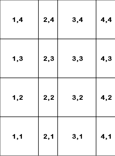
Fig. 9.2.37 Layout of a 4 by 4 cuboidal array.
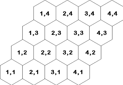
Fig. 9.2.38 Layout of a 4 by 4 hexagonal array.
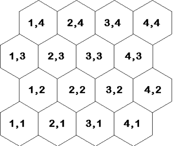
Fig. 9.2.39 Layout of a 4 by 4 stacked hexagonal (shexagonal) array.
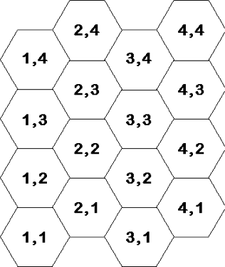
Fig. 9.2.40 Layout of a 4 by 4 rotated hexagonal (rhexagonal) array.
Although all elements of cuboidal arrays must be cuboids, they need not be the same size. Elements of each row must have the same height but may have varying widths. Similarly, elements of each column must be of a single common width but may vary in height. Less flexibility is available in hex-based arrays, because of their very nature. Hexagonal and stacked hexagonal arrays may contain only hexprisms, and all must be of the same outer size (although unit contents may vary as needed). Rotated hexagonal arrays likewise are limited to rhexprisms with a single boundary size.
9.2.4.9.2. Pin-power edits
In lattice-physics calculations, it is often necessary to obtain a pin-power edit showing the power produced in each fuel pin cell. NEWT uses the array functionality to define pin cells. When pinpow=yes is specified, an extra edit is produced that gives the normalized pin power in each pin cell. A pin cell is defined as any element within the array that contains a fissionable nuclide. Pin powers are normalized such that the average of all fuel-bearing array elements is 1.0. Array elements such as burnable poison rods or water holes, which produce no fission power, are not included in the power normalization process. The pinpow functionality is not available for hexagonal, shexagonal, or rhexagonal lattices.
Output provides an edit of each assembly for which pinpow=yes is specified. In addition, a final edit is provided for the entire system, normalized to all fuel cells in all arrays for which pinpow=yes is specified.
Pin-power edits are shown in the description of output in Sect. 9.2.6.
9.2.4.9.3. Fill operations
The final section of an array specification is the fill list. Delimited by fill and end fill keywords, NEWT expects a list of N=nux*nuy unit numbers, specifying the unit to be placed at each array position. Arrays are filled left to right, starting at the bottom left-hand corner and moving up a row after all columns in the current row are filled. In other words, any of the 4 \(\times\) 4 arrays in the figures above would be filled in the following order: (1,1), (2,1), (3,1), (4,1), (1,2), (2,2), (3,2), (4,2), (1,3), (2,3), (3,3), (4,3), (1,4), (2,4), (3,4), (4,4).
The list of elements used to fill an array consists of unit numbers. Each unit used in the fill list must be defined in the geometry block and must be of the shape and size required for the array type and position. However, NEWT provides the ability to fill an array location with a null unit, which in essence skips the current array location. This is accomplished simply by entering unit number “0” (a “null” unit) at the location to be skipped.
9.2.4.9.4. Examples of array definitions
Consider a simple 3 \(\times\) 3 square array with array ID 10, with unit 1 to be placed in the center of the array, surrounded by unit 2 cells. Such a specification would take the following form:
ara=10 nux=3 nuy=3 type=cuboidal fill
2 2 2
2 1 2
2 2 2 end fill
This may also be written spanning several lines to help visualize the layout:
ara=10 nux=3 nuy=3 type=cuboidal fill
2 2 2
2 1 2
2 2 2 end fill
Note that the array is being filled from the bottom so that the actual unit layout is inverted relative to the fill description. A fill specification that places unit 1 at the top center position in this array would be input as follows, where the second-to-last entry in the list is placed in the horizontal center of the top row.
ara=10 nux=3 nuy=3 type=cuboidal fill
2 2 2
2 1 2
2 1 2 end fill
Arrays may be nested within arrays. Each array must be placed in a unit, but a unit containing an array may be placed within another array. The following example demonstrates the use of nested arrays, along with the use of a null unit.
In this example, we define two units containing cells, a unit containing a smaller array and a global unit containing a larger array:
unit 1
'0.5/0.6 cm radius pin
cylinder 30 0.5 sides=20
cylinder 20 0.6 sides=20
cuboid 10 4p0.75
media 1 1 30
media 2 1 20 -30
media 3 1 10 -20
boundary 10 3 3

      unit 2
'0.25/0.3 cm radius pin
cylinder 30 0.25 sides=8
cylinder 20 0.3 sides=8
cuboid 10 4p0.375
media 1 1 30
media 2 1 20 -30
media 3 1 10 -20
boundary 10 3 3

'small array
unit 3
cuboid 10 1.5 0 1.5 0
array 1 10 place 1 1 0.375 0.375
media 3 1 10
boundary 10 5 5       'large array
global unit 4
cuboid 10 3.0 0.0 3.0 0.0
array 2 10 place 1 1 0.75 0.75
media 3 1 10
boundary 10 5 5
Now, in a read array block, we define array 1, a 2 by 2 array filled with unit 2 cells, and array 2, filled with two unit 1 cells, one unit 3 cell (containing array 1), and one null unit:
read array
ara=1 nux=2 nuy=2 typ=cuboidal
fill 2 2
     2 2 end fill
'
ara=2 nux=2 nuy=2 typ=cuboidal
fill 1 3
     0 1 end fill
end array
When assembled, the model would appear as shown in Fig. 9.2.41. Note that local grids override the global grid in each array location but that the global grid is seen where the null unit is placed.
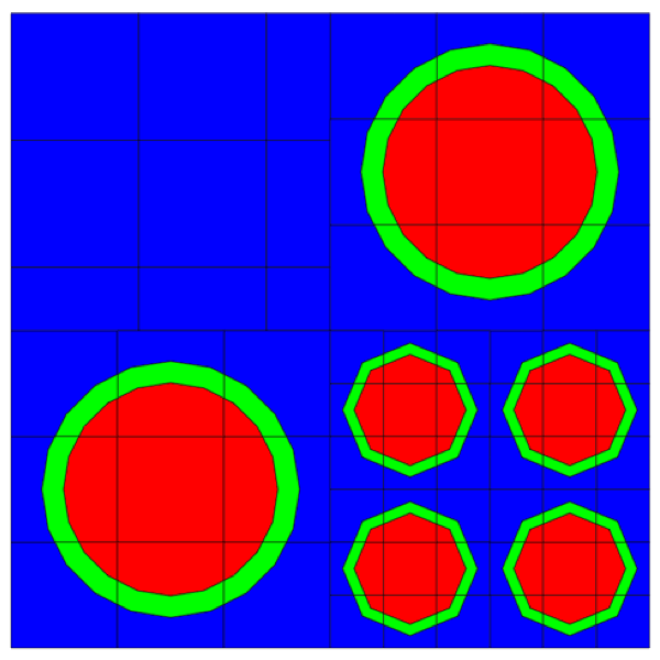
Fig. 9.2.41 Example of nested arrays and a null unit specification.
9.2.4.10. Homogenization block
Homogenization block keyword = homog, hmog, homo
As discussed earlier, NEWT can be used to collapse cross sections to a reduced broad-group format. The cross sections produced from this operation are written as microscopic cross sections for each nuclide in each mixture. NEWT also provides the ability to produce macroscopic weighted cross sections homogenized over one or more mixtures. Homogenized cross sections are created using the collapsing energy structure defined in the collapse data block or the original library’s group structure if no collapsing instructions are provided. Flux-weighted collapsed cross sections are combined with number densities and added such that reaction rates in homogenized materials are conserved.
Within the homogenization block, multiple homogenization records are permitted, and the same mixtures may be repeated in different records. Each record provides a recipe defining the mixtures to be homogenized. Homogenization records have the following form:
Homogenized     Mixture           List of         end
Mixture ID     Description    Mixtures
The homogenized mixture ID is the “nuclide” number under which the mixture is saved on the homogenized cross section library. The value is arbitrary and serves only as a means to identify the cross section set on the library, although each ID must be unique. The mixture description is an alphanumeric label of up to 12 characters that is associated with the mixture; this label provides a little more descriptive ability than the ID itself. The label may not contain blanks. Finally, the label is followed by the list of mixtures to be homogenized, terminated by the end keyword. The list may contain up to 1000 unique mixtures.
A sample homogenization block is shown below. In this illustration, two homogenized mixtures are created. This first consists of five different fuel mixtures (201–205); this could be used to obtain the average fuel cross section for an assembly containing five different fuel types. The homogenized cross sections will be written to the homogenized library as nuclide 500, with label “fuel.” The second instruction homogenizes mixtures 201, 210, and 220 from the original problem; this could be used, for example, to homogenize the fuel, clad, and moderator of a fuel pin cell. This cross section set would be written on the same library as nuclide 501, with the label “fuel_cell201.”
read hmog
500   fuel  201 202 203 204 205  end
501   fuel_cell201   201 210 220 end
end hmog
Homogenized (macroscopic) cross sections are saved in an AMPX working-format library at the unit specified by the hmoglib= parameter (default=13) [ft13f001].
Instead of calculating the sometimes complicated decay chains to determine cumulative yields, nodal codes often apply simplified models for xenon and samarium. The homogenization block therefore also enables the calculation of fitted yields for 135I, 135Xe and 149Pm for use in nodal codes. Like the Polaris sequence, NEWT relies for this calculation on a set of pre-calculated fitted yields. Up to SCALE 6.2, NEWT and Polaris used different sets of pre-calculated fitted yields. Polaris used yields that were determined based on a set of LWR Polaris calculations with subsequent yield fitting.
To improve consistency between the sequences, since SCALE 6.3, NEWT by default
uses the same fitted yields as Polaris. Yield resource lwr_yields.h5 in
SCALE’s data directory is used by both sequences. For backwards compatibility,
the yields used by NEWT up to SCALE 6.2 are available in resource legacy_yields.h5.
Users can switch the yield resource or use their own resource by linking the respective resource into the temporary working directory.
Example 1: Use NEWT legacy yield data
read shell
  cp ${DATA}/legacy_yields.h5 ${TMPDIR}/lwr_yields.h5
end shell
Example 2: Use user-defined yield data
read shell
  cp /path/to/user-resource.h5 ${TMPDIR}/lwr_yields.h5
end shell
9.2.4.11. Assembly discontinuity factors
Assembly discontinuity factor (adf) block keyword = adf
Because discontinuity factors have meaning only with respect to homogenized cross sections, ADFs are calculated only if homogenized cross sections are also specified via the Homogenization data block (see Sect. 9.2.4.10). Calculation of ADFs is specified in the read adf data block. The three supported formats of this data block are as follows. For a single-assembly model, the following format is used:
read adf
1 homg_assm_id n=Y1 s=Y2 e=X1 w=X2
end adf
For a reflected assembly model, the following format is used:
read adf
2 homg_assm_id homog_refl_id w=Xi
end adf
read adf
3 homg_assm_id line1 line2 line3 ...
end adf
where
hmog_assm_idis the identifying label assigned to the homogenized assembly,
hmog_refl_idis the label assigned to the homogenized reflector region,
Y1is the y-ordinate of the north boundary of the assembly (typically this is ymax for the global unit),
Y2is the y-ordinate of the south boundary of the assembly (typically this is ymin for the global unit),
X1is the x-ordinate of the east boundary of the assembly (typically this is xmax for the global unit),
X2is the x-ordinate of the east boundary of the assembly (typically this is xmax for the global unit),
Xiis the x-ordinate for the fuel/reflector interface,
lineiis a series of two ordered pairs (X1,``Y2``), (X1,``Y2``)that define a line segment in the NEWT grid.
In a single-assembly calculation, only a single homogenized mixture is specified. Leading index 1 indicates that ADFs for the fuel assembly are being calculated; ADFs may be calculated on any or all faces of a rectangular assembly. In a reflected assembly, the leading index is 2, followed by the homogenized mixture ID for the fuel assembly first, then the homogenized mixture ID for the reflector region. An ADF may be requested only for one location, at the fuel/reflector interface. In any configuration, ADFs may be requested for a set of arbitrary line segments defined in the NEWT geometry. In this case, the leading index is 3, followed by the homogenized mixture ID, followed by up to 12 line segments, which are defined by their beginning and ending points. ADFs along these lines are defined as the surface-averaged flux divided by the average flux defined for the associated homogenized mixture. Surface-averaged currents are also edited for each arbitrary line segment; both full and partial currents in both the x- and y- directions are provided. The net current is also provided in the few-group cross section database file xfile016. The orientation of the net current across the line segment is further discussed in Appendix A of TRITON chapter.
Although any homogenized set of mixtures can be specified for each homogenized region, the ADF will have physical meaning only if the homogenized set represents all mixtures in the assembly. Similarly, if a reflector calculation is performed, the hmog_refl_id should represent the set of homogenized reflector mixtures. The average collapsed flux in the homogenized mixtures is used to calculate the homogeneous flux for a single-assembly ADF. In a reflector calculation, the homogenized cross sections for the reflector are used to solve the multigroup diffusion approximation (Sect. 9.2.3.5).
Examples illustrate the use of the ADF input specification. Consider a 17 \(\times\) 17 pressurized-water-reactor (PWR) design. Because of symmetry, it can be modeled a \(1/4\) assembly; therefore, we choose to model the upper right quadrant, as shown in Fig. 9.2.42. Mixtures 1, 2, 3, and 4 represent the fuel, clad, moderator, and guide tube materials, respectively. The west and south sides of the model are the assembly midplanes, so ADFs calculated on these boundaries would have no physical meaning. (These are not real assembly boundaries.) However, because of the symmetry of the assembly, fluxes would be identical on all boundaries. Therefore, selection of either the north or east boundary will yield a valid ADF for all boundaries. We choose to request an ADF calculation for the east (right) side of the assembly.
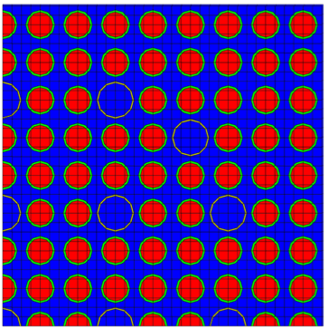
Fig. 9.2.42 Upper-right quadrant of an unreflected PWR assembly.
Assuming we are collapsing 44 energy groups to 2 energy groups, we would specify the following collapse, homog, and adf blocks to obtain 2-group ADFs representative of this assembly:
read collapse
22r1 22r2
end collapse
read hmog
500 assm   1 2 3 4 end
end hmog
read adf
1 500 e=10.752
end adf
Again, recall that for a single assembly, the ADF in each energy group is simply the average flux on the specified boundary divided by the average flux for the entire assembly, which in this case is the flux in homogenized mixture 500.
ADF can also be calculated using the arbitrary line-segment ADF type. Using this new ADF type, the ADF input would be the following:
read collapse
22r1 22r2
end collapse
read hmog
500 assm   1 2 3 4 end
end hmog
read adf
3 500 10.752 0.0 10.752 10.752
end adf
In this example, the east-side ADF will be calculated along the line segment starting at (10.752,0) and ending at (10.752,10.752). The values of the line segments depend on a coordinate system of the global unit.
For a reflected model, consider the same type of assembly but representing an assembly placed on the core periphery. It is bounded on one side by a 2 cm stainless steel baffle and 10 cm of water, beyond which is treated as vacuum. Because the reflector calculation is a 1-D solution, it is not possible to directly model a fuel assembly with two reflector boundaries. Typically the assumption is made that the same ADF may be applied in any assembly/reflector boundary and that a 1-D reflector model is all that is necessary. This model is pictured in Fig. 9.2.43. Notice that different mixtures are used in the reflector model. Fluxes used in homogenized mixtures and for generating homogenized cross sections are spatially averaged; thus, it is important to separate the moderator in the reflector from that in the fuel assembly such that average fluxes in each region properly characterize that region. For example, the flux in the reflector will be significantly different (far more thermal) from the flux within the assembly.
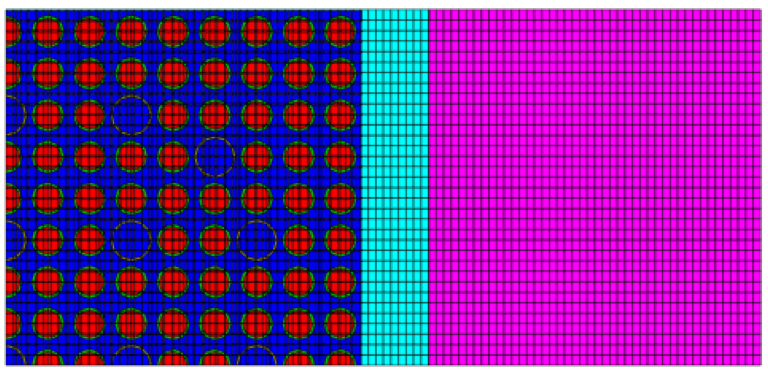
Fig. 9.2.43 Upper-right quadrant of a PWR assembly with baffle and reflector.
Assuming again a collapse from 44 energy groups to 2, the following collapse, homog, and adf blocks would be specified to obtain 2-group ADFs representative of the assembly and the reflector; 2-group cross sections for each homogenized region would also be prepared from the collapse and homogenization instructions:
read collapse
22r1 22r2
end collapse
read hmog
500 assm   1 2 3 4 end
501 reflector 5 6 end
end hmog
read adf
2 500 501 w=10.752
end adf
9.2.4.12. Flux planes
Fluxplane block keyword = fluxplane, fluxplan, flux, fluxplanes
The fluxplane block is a special output edit that lets one obtain the average scalar flux and currents along any line segment or any continuous set of collinear line segments. One must simply specify the start and end points of a line segment for which a linearly averaged flux is desired. This line segment must correspond to one or more line segments in the model’s grid structure, which requires some knowledge of where grid lines exist in the model.
The format of a flux plane specification is as follows:
read fluxplane
text_label homg_assm_id xstart ystart xend yend
…
end fluxplane
where text_label is an alphanumeric description used to label the selected plane in the output, homg_assm_id is the identifier in the homog block, and (xstart, ystart) and (xend, yend) are the start and end points, respectively, for the line segment for which an average flux is desired. The text_label string must not contain white space and may be up to 16 characters in length.
As an example, we consider a simple model consisting of two dissimilar pin cells (1/4 cells):
global unit 1
cuboid 1 1.26 0.0 0.63 0.0
cylinder 2 .4750 chord +x=0 chord +y=0 sides=20
cylinder 3 .4095 chord +x=0 chord +y=0 sides=20
cylinder 4 .6030 chord +y=0 chord -x=1.26 origin x=1.26 sides=20
cylinder 5 .5630 chord +y=0 chord -x=1.26 origin x=1.26 sides=20
media 1 1 3
media 2 1 2 -3
media 10 1 5
media 2 1 4 -5
media 3 1 1 -2 -4
boundary 1 4 2
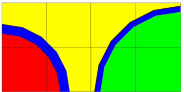
We know a line segment (actually, two) exists at x = 0, x = 0.63, and x = 1.26, between y = 0 and y = 0.63. Thus, a legitimate set of flux plane specifications would be the following:
read fluxplane
cell_interface 0.63 0.0 0.63 0.63
midplane_cell1 0.0 0.0 0.0 0.63
midplane_cell2 1.26 0.0 1.26 0.63
end fluxplane
This will provide a summary of fluxes and currents at each line segment in fine-group structure, and if a collapse is performed, in broad-group structure. Results from a calculation with a two-group collapse appear as follows:
Broad Group Fluxes:
 Group    cell_interface    midplane_cell1    midplane_cell2
    1      5.906586D+01      5.903113D+01      5.930420D+01
    2      7.645792D+00      7.641424D+00      6.705809D+00

Broad Group Currents (x):
 Group    cell_interface    midplane_cell1    midplane_cell2
    1     -3.481505D-01      0.000000D+00      0.000000D+00
    2      3.004759D-01      0.000000D+00      0.000000D+00

Broad Group Currents (y):
 Group    cell_interface    midplane_cell1    midplane_cell2
    1      1.081450D-01      1.652161D-01      1.120160D-01
    2     -1.031163D-01     -1.647396D-01     -9.993214D-02
Output also includes +x, -x, +y, and -y components of currents.
9.2.4.13. Mixing table block
Mixing table block keyword = mixt, mixtable
Generally, NEWT calculations are performed using a cross section library and mixing table prepared in advance by other SCALE modules. However, NEWT allows the user the ability to manually specify the isotopic composition of each mixture used in a NEWT model. If a mixing table block is read, any existing mixing table data file is ignored. Therefore, all mixtures specified in the material block must be mixed in the mixing table block.
The format of the mixing table is simple and straightforward. For each nuclide used, three parameters must be supplied: (1) mixid, the mixture ID number into which the nuclide is to be mixed; (2) nuclideid, the SCALE ID number for the nuclide (which must exist on the cross section library being referenced); and (3) concentration, the number density (atoms/b-cm) of the nuclide in this mixture. The same nuclide may appear in multiple mixtures or more than once in a single mixture if desired. Macroscopic cross sections are determined for each mixture by the following formula:
where
\(\Sigma^{R}\) is the mixed macroscopic cross section for reaction R in the mixture,
Ni is the number density of nuclide i,
\(\sigma_{i}^{R}\) is the microscopic cross section for reaction R in nuclide i.
The form of the mixing table block is as follows:
read mixt
mixid1 nuclideid1 concentration1
mixid2 nuclideid2 concentration2
mixid3 nuclideid3 concentration3
…
mixidN nuclideidN concentrationN
end mixt
This concludes this list of input blocks available within NEWT. The following section provides a list of sample inputs used to represent a variety of configurations and use of codes. These examples are intended to provide a broader illustration of the use of NEWT in a range of potential applications.
9.2.5. Examples of Inputs
This section provides annotated sample input listings for three different model types, showing the use of a number of different options and approaches in model development for a variety of applications. These samples use the TRITON T-XSEC sequence to prepare cross sections for stand-alone NEWT calculations. In general, this is more easily accomplished as a TRITON T-NEWT calculation in which cross section processing and a NEWT transport solution are combined into a single calculation. However, the user is directed to the TRITON user’s manual (Chapter T1.4 of the SCALE manual) for details on T-XSEC and T-NEWT calculations. The examples are intended simply to demonstrate the use of the NEWT code. The T-XSEC data are included to allow a user to observe the mixture definitions used in the NEWT input in its calculation. These problems are also available as sample problems in the SCALE distribution.
9.2.5.1. Sample 1
Sample 1 illustrates the use of a series of three consecutive stand-alone NEWT calculations. Annotated input for this problem is given in Fig. 9.2.44. The calculation begins with SCALE standard composition specifications used to prepare a problem-specific weighted cross section library and mixing table for use by NEWT. In this case the T-XSEC sequence of the TRITON control module is used. This input is described in the TRITON chapter and is not described further here.
The first NEWT case uses no parameter block; thus, all default parameters are applied. The default is an eigenvalue calculation, with cross sections read from ft04f001 (xnlib=4) and collapsed cross sections written to ft30f001 (wtdlib=30). The 238-group cross section library is collapsed to a 44-group library using mixture-weighted fluxes. The model calculates the eigenvalue for a simple 1/4 pin cell. The center of the pin is placed at the origin, the lower-left corner of the global unit boundary, inlaid into a 2 by 2 base grid. The grid structure is illustrated in Fig. 9.2.45.
The second case performs the same calculation using the collapsed cross section library created by the first case. Parameter restart=no is set to prevent the code from attempting a restart from the existing library. Because the first case saved 238-group fluxes and the second case uses 44 energy groups from the collapsed set, a restart is not possible.
The third NEWT case is a calculation identical to the second case, although the input is different. In this case, the flux restart file from the previous calculation is used as a first guess for fluxes. This is permitted since both cases used the same cross section library and therefore have the same energy boundaries. For this case, the “read geom” data block is omitted, telling NEWT to use the geometry restart file from the previous case. This allows a rapid restart, since no geometric data need to be recomputed. Because no other parameters are changed, this case will converge after one outer iteration to the same eigenvalue as in the first case.

Fig. 9.2.44 Sample 1 input listing (annotated).
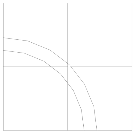
Fig. 9.2.45 Grid structure for 1/4 pin cell of Sample 1.
9.2.5.2. Sample 2
Sample 2 (shown in Fig. 9.2.46 and Fig. 9.2.47) illustrates the use of multiple bodies within a single unit. It highlights the use of media definitions to include and exclude regions when various bodies are used. Although an array can be used to place bodies, this example illustrates a method suitable for use in developing a model for a configuration with an irregular non-array-type structure. This sample problem also highlights the use of partial-current unstructured-mesh CMFD acceleration, which reduces the number of outer iterations from 35 to 21 and the CPU run time by ~25%.

Fig. 9.2.46 Sample 2 input listing (annotated).
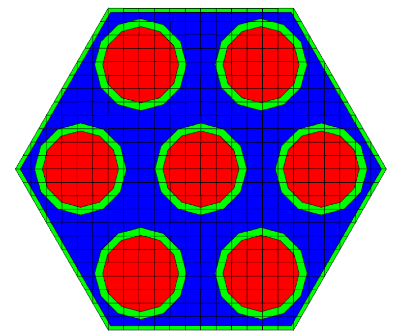
Fig. 9.2.47 Mixture placement and grid structure for model described in Sample 2.
9.2.5.2.1. Sample 3
Sample 3 demonstrates the development of a VVER-440 hexagonal fuel assembly. Annotated input for this problem is given in Fig. 9.2.48. The output plot for this model is shown in Fig. 9.2.49. The key attributes of this model are as follows:
the use of hexagonal (hexprism) units in a stacked hexagonal array,
the use of null units as placeholders in the array,
a full model within a rhexagonal outer boundary,
the use of white boundary conditions,
- the use of the new partial-current-based unstructured CMFD
acceleration for hexagonal-domain configurations, and
new type-3 ADF inputs.
Using CMFD acceleration, the number of outer iterations needed for convergence decreased from 21 to 8 with a run-time speedup of ~2.58.

Fig. 9.2.48 Sample 3 input listing (annotated).
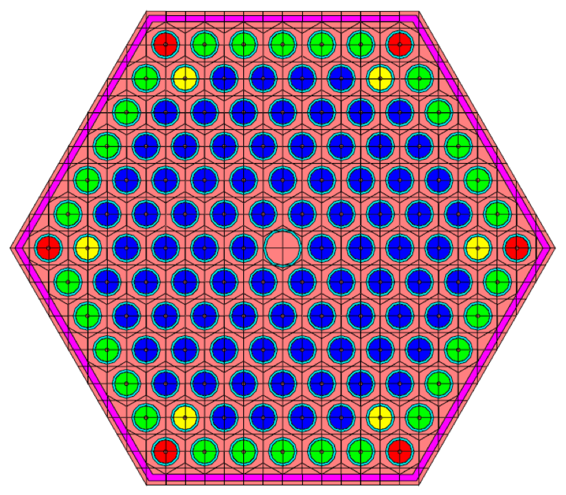
Fig. 9.2.49 Grid structure and material placement for VVER-440 model.
9.2.5.3. Sample 4
Sample 4 demonstrates the use of NEWT in modeling a larger, more complex configuration. Annotated input for this problem is given in Fig. 9.2.50. The calculation begins with the use of SCALE standard composition specifications to prepare a problem-specific weighted cross section library and mixing table for use by NEWT. In this case the T-XSEC sequence of the TRITON control module is used.
This NEWT case is used to calculate the eigenvalue of an infinite lattice of fuel assemblies. Symmetry at the assembly center is used to reduce a 15 by 15 assembly lattice to a smaller one-quarter assembly. The grid structure is illustrated in Fig. 9.2.51. A similar illustration showing media placements by color is given in Fig. 9.2.52.
This input illustrates several features of NEWT modeling capabilities. Some important features of this model are as follows.
In this sample problem, S-6 quadrature, P-1 scattering (P-2 in the moderator), spatial convergence criteria of 0.005, and an eigenvalue convergence criteria of 0.001 are used. These are an order of a magnitude larger than the values typically used for LWR lattice calculations.
Two sets of UO2 cross sections are prepared in the T-XSEC calculation. These cross sections are identical with the exception of the mixture number. Since NEWT reports fluxes, reaction rates, etc., by mixture, the placement of a unique mixture at a specific location in a model allows one to determine, for example, the reaction rates at that model location. Mixture 7, placed in unit 9 in this model, occurs in only one pin location in the model. Mixture 1, placed in all other fuel rod locations, will yield reaction rates close to the average of those for all fuel in the assembly. If the flux or reaction rate was needed in each unique fuel location, a unique mixture would be needed for each location.
The use of chords for cutting cylinders allows inclusion of one-half and one-quarter fuel cells in the quarter-assembly model. Because the fuel assembly has an odd number of rods in each dimension, use of symmetry at the assembly midplanes requires the rods to be bisected.
In this model, local grid spacing was selected such common grid spacings occur in all cells. However, this is not a requirement. For example, a much more refined local grid could have been specified for unit 9. There is no requirement that grid lines match between different elements of an array.
Unstructured coarse-mesh finite-difference acceleration (cmfd=2 or cmfd=yes) was employed to accelerate the convergence of the solution. For this case, 14 outer iterations were required for full spatial convergence as compared with 30 outer iterations when CMFD is disabled. The CMFD-accelerated case ran 2.5 times faster than its unaccelerated counterpart. In this sample problem, xycmfd=2 was used to define the coarse-mesh grid to have two fine-mesh cells per coarse-mesh cell.
Two-group homogenized cross sections were generated along with single-assembly (i.e., type 1) ADFs derived from the Collapse block, ADF block, and the Homogenization block. In addition, a B1 critical spectrum search is computed after the transport calculation, which is folded into the transport solution to generated homogenized constants.

Fig. 9.2.50 Sample 4 input listing (annotated).
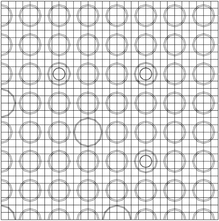
Fig. 9.2.51 Grid structure for one-quarter assembly of Sample 4.
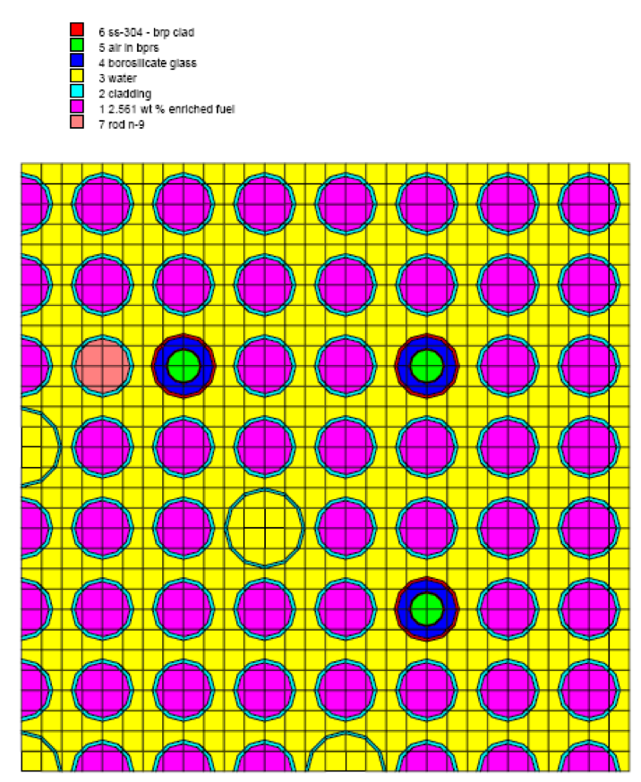
Fig. 9.2.52 Mixture placement for quarter-assembly model of Sample 4.
9.2.5.4. Sample 5
Sample 5 (Fig. 9.2.53) illustrates a calculation for a fuel assembly with a large water boundary and a vacuum boundary condition. The calculation begins with the use of SCALE standard composition specifications to prepare a problem-specific weighted cross section library and mixing table for use by NEWT.
In this model, seven UO2 pins are adjacent to eight MOX pins, which, in turn, are adjacent to a large reflector region. The outer boundary of the reflector is vacuum. Reflection on the top and bottom boundaries makes the problem infinite in the y direction. The grid structure for this problem is illustrated in Fig. 9.2.54. This problem illustrates the use of the original CMFD acceleration scheme in NEWT (cmfd=1 or cmfd=rect). Because of the large degree of scattering within the reflector region, the problem can be relatively slow to converge. Without CMFD acceleration, 40 outer iterations are required for spatial convergence as compared with 12 when CMFD is enabled. A total run-time speedup of ~1.4 is achieved with the CMFD acceleration scheme.
In addition to the application of CMFD, Sample 5 also illustrates the use of NEWT’s reflector ADF capability. Reflector ADFs are computed along the fuel/reflector interface.

Fig. 9.2.53 Sample 5 input listing (annotated).

Fig. 9.2.54 Grid structure for 15-pin row of Sample 5.
9.2.6. Description of Output
This section contains a brief description and explanation of NEWT output. Portions of the output will not be printed for every problem. Some output is optional, depending on user input specifications and is so noted in the description. As with any SCALE module, output begins with an input echo, module execution records with times and completion codes, and the program verification information banner page. These outputs are common to all SCALE modules and are not described here.
9.2.6.1. NEWT banner
Following the SCALE program verification information, the first section unique to NEWT output is the NEWT banner, which appears as shown in Fig. 9.2.55. The bottom of the banner gives the title of the case as given in input. The NEWT banner is printed only if the command line option -p is used to run SCALE.
Fig. 9.2.55 NEWT copyright banner page and case title.
9.2.6.2. Input summary
The next several pages of output provide a summary of input parameters. As described in Sect. 9.2.6, default parameters are used when no user specification is supplied. The input summary lists all parameters and states used in the calculation, whether user supplied or default. The following subsections describe the various blocks of output information provided in the input summary.
9.2.6.2.1. Control options
The Control Options block lists global control parameters that determine the type of analysis being performed. A sample Control Options page is shown in Fig. 9.2.56. Parameters are self-explanatory. More information is available in the description of the keywords in Sect. 9.2.6.2.

Fig. 9.2.56 Control Options page.
9.2.6.2.2. Output options
The Output Options block (Fig. 9.2.57) lists selections made for output. Portions of the output listing will be printed only if the appropriate printing option was selected.

Fig. 9.2.57 Output Options page.
9.2.6.2.3. Input/output unit assignments
The Input/Output (I/O) Unit Assignments block (Fig. 9.2.58) simply lists the unit numbers selected for reading or writing various data files, as appropriate for the calculation.

Fig. 9.2.58 Input/Output Unit Assignments page.
9.2.6.2.4. Convergence control parameters
The Convergence Control block (Fig. 9.2.59) summarizes all parameters used to control spatial, angular, and eigenvalue convergence for the iterative phases of the solution process.

Fig. 9.2.59 Convergence Control Parameters page.
9.2.6.2.5. Pin-power edit requests
If pin-power edits are requested for one or more arrays, a listing is provided of the arrays for which this request was made (Fig. 9.2.60).

Fig. 9.2.60 Pin-power edit request summary.
9.2.6.2.6. Geometry specifications
The Geometry Specifications block (Fig. 9.2.61) lists parameters associated with the geometric model specified by the user. The first section lists the characteristics of the global unit. This is followed by a listing of the four boundary conditions. Finally, the last section in this block lists all bodies specified for the model. The appearance and contents of this section of input depend on the nature of the input model.

Fig. 9.2.61 Geometry Specifications page.
9.2.6.2.7. Homogenization region specifications
The Homogenization Region Specifications block (Fig. 9.2.62) summarizes all sets of homogenized cross sections requested in user input.

Fig. 9.2.62 Homogenization Region Specifications page.
9.2.6.2.8. Material specifications
The Material Specification block (Fig. 9.2.63) lists the NEWT material number, counting in the order read in; the SCALE mixture number; and the Pn order assigned for that mixture.

Fig. 9.2.63 Material Specifications page.
9.2.6.2.9. Derived parameters
The Derived Parameters block (Fig. 9.2.64) lists values not specifically input but derived from other sources of input. Some of this information comes from the cross section library, some from the model geometry, and some from the Sn and Pn values specified.

Fig. 9.2.64 Derived Parameters page.
9.2.6.2.10. Energy group structure listing
The Energy Group Structures block (Fig. 9.2.65) lists the energy and lethargy boundaries found in the cross section library. If a broad-group collapse was requested, the boundaries of the broad-group library that will be produced are also identified. This example shows the structure of the SCALE 44GROUPNDF5 library and 2-group fast/thermal collapse structure. The final entry (group 45, broad group 3) indicates the lower bound of the previous energy group.

Fig. 9.2.65 Energy Group Structure Listing page.
9.2.6.2.11. Quadrature parameters
The Quadrature Parameters block (Fig. 9.2.66) lists the first-quadrant angles and weights used for the specified order of quadrature. The same angles and weights are applied in the other three quadrants; however, the signs of the angles vary with the quadrant. Also listed are the Pn moments associated with the maximum Pn scattering order requested in all materials. Of course, only a subset of these moments applies to the lower-order Pn assignments.

Fig. 9.2.66 Quadrature Parameters page.
9.2.6.2.12. Mixture volumes listing
The Mixture Volumes block (Fig. 9.2.67) provides a summary of the volume and volume fraction of each mixture in the problem, together with the total volume. This block can be used as a simple check of the input model by ensuring that the calculated volumes of mixtures used for a given problem match the expected volumes or volume fractions.

Fig. 9.2.67 Mixture Volumes page.
9.2.6.2.13. Mixing table listing
The Mixing Table block summarizes the input mixing table, whether user supplied or read from a SCALE-generated file. Number densities are in units of atoms per barn-centimeter. Although optional, the mixing table is printed by default. This default setting can be disabled by specifying prtmxtab=no in the Parameter block. A sample mixing table is shown in Fig. 9.2.68.

Fig. 9.2.68 Mixing Table Listing page.
9.2.6.2.14. Nuclide cross sections
The Nuclide Cross Section block is optional and is printed only when prtxsec=yes is specified in the Parameter Block. The volume of output generated is quite extensive, especially when a very fine group library is used and/or a large number of nuclides are included in the mixing table. The nuclide data are taken directly from the working library used for the calculation. A sample showing a partial listing for a single nuclide is shown in Fig. 9.2.69.
Following the block header, nuclide data are listed for all nuclides. For each record, the same format is used. Nuclide data begin with a listing of nuclide header information. This is followed by a listing of the 1-D cross sections that are important in NEWT calculations. The sample below shows a partial listing of the 1-D cross sections. Following the 1-D cross section listing is the scattering matrix for the nuclide. This abbreviated listing shows a portion of the P0 matrix for this nuclide; however, in a full listing, all higher-order elements are printed as well.
As was indicated in the input description, specification of prtxsec=1d can be used to obtain header and 1D cross section data only, skipping the printing of scattering matrices.

Fig. 9.2.69 Partial listing of Nuclide Cross section data pages.
9.2.6.2.15. Mixture cross sections
The Mixture Cross Section block provides mixed macroscopic cross sections for each mixture provided in the input mixing table. The block is also optional and is printed only when prtmxsec=yes is specified in the Parameter Block. Although the volume of output generated is not as extensive as that of the nuclide listings, the mixture cross section print can be voluminous, especially when a very fine group library is used and/or a large number of mixtures are included in the mixing table. A sample showing a partial listing for a single mixture is shown in Fig. 9.2.70.
Following the block header, information is provided for each mixture using the same format. Mixture data begin with a listing of general mixture information, including the mixing table for that mixture. This is followed by a listing of 1-D cross sections important in NEWT calculations. The sample below shows a partial listing of the 1-D mixed macroscopic cross sections. Following the 1-D cross section listing is the scattering matrix for the nuclide for all moments requested for the mixture. This abbreviated listing shows a portion of the P0 matrix for this nuclide; however, in a full listing, all higher-order elements are printed as well if greater than P0 scattering was requested.
As was indicated in the input description, specification of prtmxsec=1d can be used to skip the printing of scattering matrices.

Fig. 9.2.70 Partial listing of Mixture Cross section data pages.
9.2.6.3. Iteration history
The next portion of NEWT output lists the iteration convergence history for the iterative solution (Fig. 9.2.71). This information can be used to track and understand the performance of the outer loop of the iterative solution. The first column provides the outer iteration count. The second column lists the system eigenvalue after each outer iteration. The third column lists the change in the eigenvalue from the last outer iteration; this is one of the parameters tested for convergence. The fourth column, “Max Flux Delta,” gives the maximum change in cell flux for all cells and all energy groups; this is also used as a convergence test. The next column lists the cell number and energy group corresponding to the maximum flux change in this iteration. The next two columns list the same flux information for mixtures with fissionable nuclides. This can be used to track spatial convergence in fuel when convergence is slowed by significant scattering outside the fuel. Finally, the last column provides information on the convergence of inners in each outer iteration. Inner iterations do not need to converge within early outer iterations, but final convergence will not be achieved until all inners are converged. The maximum number of inner iterations per energy group is set by the inners= parameter in the parameter input block. After convergence is achieved, the table is terminated by printing the final version of keff.
If the parameter keyword timed= is set to yes, four additional columns are introduced that give timing information on the solution process, listing real (“wall clock”) time, elapsed CPU time since beginning the iteration process, elapsed CPU time per outer iteration, and an estimate of the fractional CPU usage during each outer. Fig. 9.2.72 illustrates the form of output produced when timed=yes is input. Additionally, a supplementary edit follows the iteration edit when timed=yes, giving information on average time per transport sweep (outer iteration) within different components of the solution. This edit is especially useful when coarse-mesh finite-difference acceleration is used, to assess the overhead of the CMFD accelerator.

Fig. 9.2.71 Nominal iteration history output.

Fig. 9.2.72 Timed iteration history output.
9.2.6.4. Four-factor formula
Following the iteration history listing, NEWT output provides edit listing the four traditional components of the four-factor formula. This is followed by an alternate three-group formulation that separates out resonance and fast escape probabilities (Fig. 9.2.73).

Fig. 9.2.73 Four-factor formula with alternate three-group formulation.
9.2.6.5. Fine-group balance tables
Following the iteration history and flux convergence, a fine-group balance table is provided for each mixture used in the calculation. Fine group refers to the group structure of the library used for the calculation. Broad-group data, discussed later, refer to a group structure collapsed from the original fine-group structure. After tables for all mixtures are printed, a last table provides a fine-group summary for the entire problem (i.e., the volume-weighted average for all mixtures). Balance tables are printed by default but may be disabled by setting prtbalnc=no in the Parameter block.
Fig. 9.2.74 shows a clipped excerpt from the fine-group summary of an output listing. Similar tables are produced for each mixture in the problem for all energy groups in the problem. The header lists the NEWT mixture number; the mixture ID (i.e., the SCALE mixture number); and the mixture description, if provided in the original input specification. The header also gives the number of computational cells in which the mixture was present and the volume of the mixture in the problem.
For each mixture, two tables are printed. The first table provides a balance of all sources and loss terms: the fixed source, the fission source, in-scatter, out-scatter, absorption, leakage, n-2n production, and the net balance of all terms for each energy group. The final row lists the mixture total for all groups. The fixed source lists the user-supplied source for fixed-source problems. This field is disabled (set to zero) for eigenvalue calculations. The fission source is the number of neutrons born into each energy group in the mixture. In this example, the mixture is water, which is not fissile; hence, no fission source is present. In-scatter represents the number of neutrons scattered into each group from all other groups; conversely, out-scatter is the loss from each energy group by scattering. Absorption is the number of neutrons absorbed in reactions that do not emit a neutron (e.g., n-\(\gamma\)). Leakage is the net loss of neutrons from the mixture to another mixture or a nonreflective boundary, and n-2n is the effective n-2n production rate calculated from a weighted sum of all n-xn reactions. The balance table is the ratio of production to loss in each energy group.
The second fine-group balance table, also shown in Fig. 9.2.74, lists other reactions rates of interest. The first two columns after the group number list in-scatter broken into its upscatter and downscatter components. The subsequent two columns provide a similar breakdown for out-scatter from the energy group. Self-scatter is the amount of within-group scattering occurring within each energy group. The fission rate is the number of (n-fission) reactions occurring in each group. The next column provides the transverse leakage (i.e., the product of the flux and the DB2 term). This column will provide only nonzero values when a nonzero buckling height is specified in input. The final column lists the total (scalar) flux for each energy group.

Fig. 9.2.74 Partial mixture fine-group balance table output.
9.2.6.6. Planar fluxes and currents
If planar fluxes are requested, an edit is printed to provide fluxes and currents on each line segment specified, identified by label (Fig. 9.2.75). Fine-group fluxes are listed for each energy group, followed by x and y net currents and partial currents (+x, -x, +y, and -y). Fluxes and currents are printed for each group in the input group structure. The example below shows only partial listings of each for simplicity. If a broad-group collapse is requested, the fine-group output is followed by the set of fluxes and currents for each broad energy group.
Note that discontinuity factors make internal use of planar fluxes to determine the flux and current on each boundary. Hence, planar flux edits will be present any time an ADF calculation is performed.

Fig. 9.2.75 Example of planar flux and current output (continued below).

9.2.6.7. Pin-power edits
The next section of the NEWT output listing is the pin-power edit (Fig. 9.2.76). This information is printed only if pinpow=yes is set in one or more arrays. Two maps are provided. The first is the power of each fuel location relative to all other fuel pins in all other arrays for which pinpow=yes. This is useful if multiple fuel assemblies are present or if more than one array is used to describe a fuel assembly. The second power map shows the pin edit normalized to the set of pins within the single array. Both maps are identical in a relative sense; different normalization factors are applied. If pinpow=yes is specified for only one array, then the two edits will have the same normalization factor and will be identical. The location of each pin is identified by the (x,y) coordinate of the center of each element of the array, in centimeters. Please note that the pin-power option is available only for square (cuboidal) arrays.
Following the two maps is a one-line edit identifying the location and magnitude of the maximum pin power.

Fig. 9.2.76 Example of pin-power edit.
9.2.6.8. Broad-group collapse
9.2.6.8.1. Broad-group summary data
The next section of the NEWT output listing is the broad-group summary listing (Fig. 9.2.77). This is printed only if a broad-group collapse is performed. This section lists broad-group data calculated based on the collapsing scheme applied. First, the energy group structure is printed, followed by cell-averaged fluxes in each mixture, for all collapsed groups. This is followed by flux disadvantage factors for each mixture and each broad group.
Note that when NEWT is used as the transport solver within TRITON depletion calculations, a three-group collapse is always done automatically. If a second user-specified collapse is requested, broad-group summary data will be provided for both collapsing structures.

Fig. 9.2.77 Broad-group summary output.
9.2.6.8.2. Broad-group cross section data
The next section of data in a NEWT output listing is the broad-group cross section output (Fig. 9.2.78). This is printed only if a broad-group collapse is performed and if prtbroad=yes is specified in Parameter block input. This block lists the collapsed cross section data for key reactions for each nuclide used in the calculation. This is a summary form of the data that are written to the collapsed cross section library. It does not list all reactions. Such data may be read directly from the working-format library by other SCALE utilities if needed. The listing below shows the data printed for a single nuclide. Data are written in the same format for all nuclides used in the analysis.

Fig. 9.2.78 Partial broad-group cross section listing.
9.2.6.9. Critical spectrum edit
When a critical buckling correction is requested (e.g., solntype=b1 is set in the NEWT parameter block or user-defined material buckling or transverse height), the critical spectrum is computed using either the B1 approximation or the P1 approximation (Fig. 9.2.79). The output lists the buckling in 1/cm2, the method (B1 or P1), and the computed critical spectrum as a function of energy. Note that the spectrum is normalized “per unit lethargy” to be equal to 1.0. In addition to the critical spectrum, the critical adjoint spectrum and the zero-buckling spectra (forward and adjoint) are also edited.

Fig. 9.2.79 Partial collapsing spectra listing for a case with critical buckling correction.
9.2.6.10. Assembly discontinuity factors
When calculation of assembly discontinuity factors (ADFs) is requested, a broad-group edit is provided for each face for which an ADF was selected (Fig. 9.2.80). Up to four ADFs may be printed for the fuel region. If the model contains a reflector region in addition to the required fuel region, then ADFs are printed for a single face, typically the fuel/moderator interface. Discontinuity factors for user-input surfaces may also be edited.

Fig. 9.2.80 Output of assembly discontinuity factors.
9.2.6.11. Groupwise form factors
Whenever homogenization is performed and pin-power edits are requested, NEWT will automatically calculate groupwise form factors (GFFs). GFFs are used in pin-power reconstruction calculations for homogenized assemblies used in nodal diffusion methods (Fig. 9.2.81).

Fig. 9.2.81 Partial collapsing spectra listing for a case with no critical buckling correction.
9.2.6.11.1. Homogenized cross sections
When homogenization is performed and parameter prthmmix=yes is set, the final output section of a NEWT calculation is the homogenized cross section edit, as shown in Fig. 9.2.82. This information is generally passed to nodal analysis codes and hence is presented in a slightly different format from other cross sections. Output includes a region-averaged k-infinity value, transport-corrected cross section, and two interpretations of absorption. The first is the directly collapsed absorption cross section, while the second (Total-Scatter) is a more consistent definition of absorption as applied in nodal calculations. The difference between the two definitions is the effective (n-2n) cross section. Both cross sections exclude contributions from 135Xe and 149Sm; microscopic cross sections and number densities for these two nuclides are printed explicitly elsewhere in the table. Nu*fission is the product of the fission cross section and the number of neutrons produced per fission, while Kappa*fission is the product of the fission cross section and the energy release per fission (J). Inverse velocity is the inverse (1/x) of the group neutron speed.
The table also lists the two-group isotropic scattering matrix and the prompt fission fraction distribution. Finally, NEWT lists approximate six-group decay constants (lambdas) and group fractions (betas) for each group.
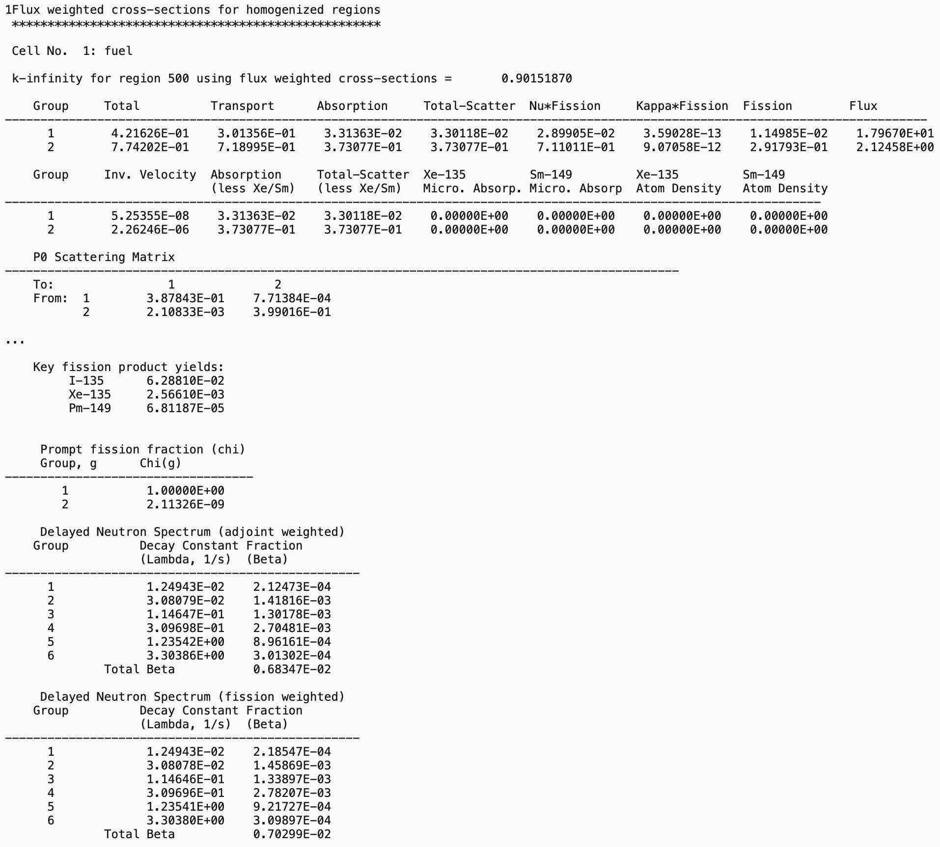
Fig. 9.2.82 Homogenized cross section edit for nodal diffusion applications.
9.2.6.12. End-of-calculation banner
NEWT output listings are terminated with an end-of-calculation banner (shown in Fig. 9.2.83) upon successful completion of a calculation. If this banner is not present, then the calculation ended abnormally, and the output listing must be reviewed to determine the cause of the error. In general, the final lines of an output file describe the error condition that caused the calculation to stop.

Fig. 9.2.83 End-of-calculation banner listing.
9.2.6.12.1. Postscript graphics files
Two user-selectable options within NEWT provide the ability to generate
PostScript-based graphics files for visualization of both input
specifications and output results. By specification of drawit=yes in
the NEWT parameter block, NEWT will generate two PostScript-based plot
files: newtgrid.ps and newtmatl.ps. The former, a grayscale plot of the
line segments generated by NEWT based on the input specification, will
be generated if all body placement input is valid. If input contains
errors such that the code stops before grid generation routines are
completed, no newtgrid.ps output is created.
The newtmatl.ps plot illustrates the same grid structure but with
material placement indicated by color. At this time, no user control is
provided for color assignment or plot control. This plot also requires
complete grid generation; additionally, it requires completion of all
media placement routines before the plot will be produced.
Figures used throughout this manual were generated from newtgrid and
newtmatl PostScript plot files. Files newtgrid.ps and newtmatl.ps are
automatically copied back from SCALE’s temporary directory to the
original location of the input case, with the names
casename.newtgrid.ps and casename.newtmatl.ps.
When prtflux=yes is input, NEWT will generate a set of flux plots showing relative neutron number densities in each energy group. A plot file will be generated with the name fluxplot_Ng.ps, where N is the number of energy groups in the problem. If an energy collapse is performed, an additional file named fluxplot_Mg.ps is created, where M is the number of energy groups in the collapsed set. Fig. 9.2.84 is an example of a flux plot output for the fast group of a two-group flux collapse.
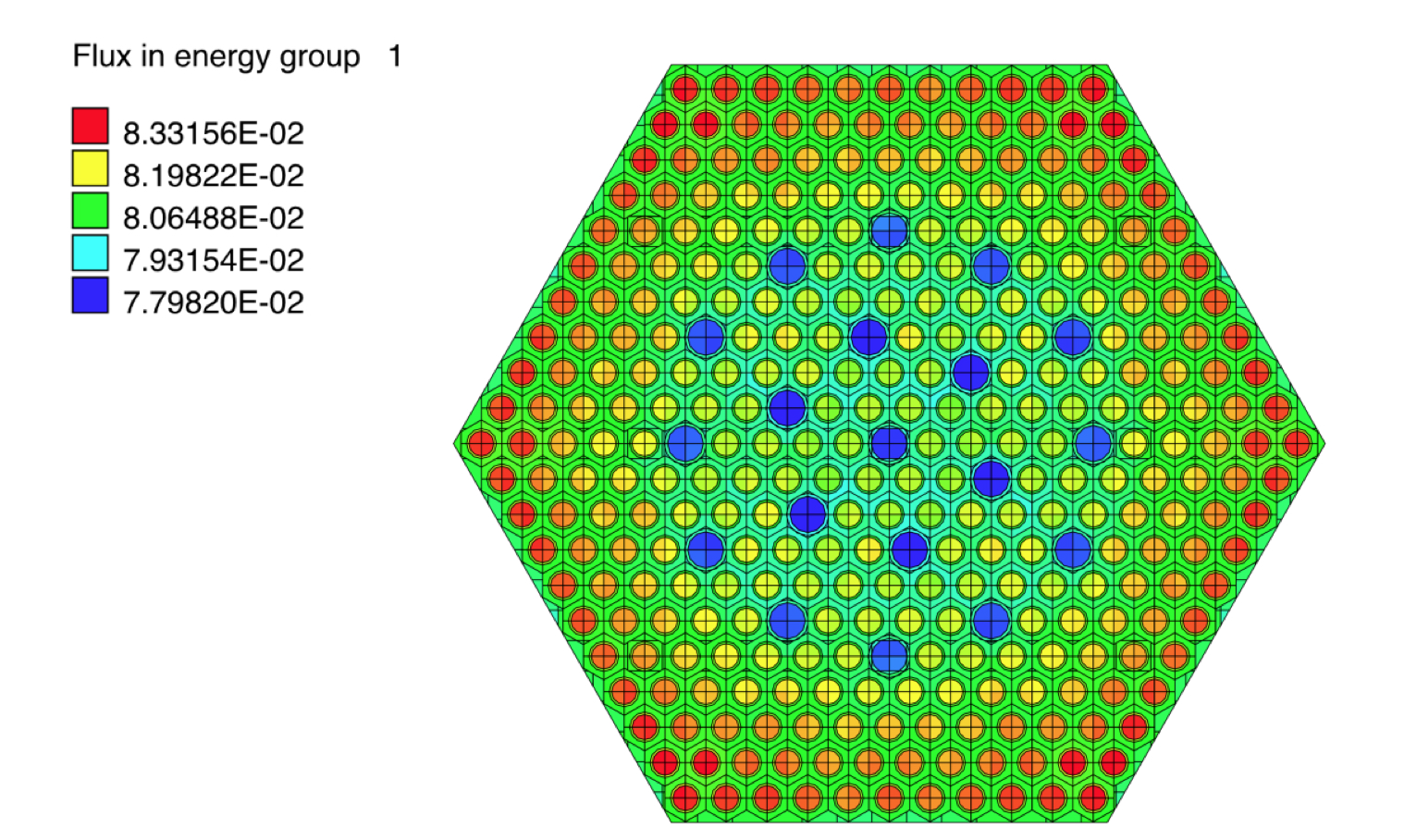
Fig. 9.2.84 Example of a flux plot image created with prtflux=yes.
9.2.6.13. Media zone edits
NEWT automatically determines “zones” representing spatially independent regions of the same media. For example, in a fuel pin cell, the fuel, clad, and moderator are all considered separate zones. In an array of such pin cells, each unique location is a unique zone. Zone numbers and the geometric location of each zone are listed in the Geometry Specification” in Sect. 9.2.6.2.6.
Upon completion of a calculation, NEWT provides an output edit of each zone by number, giving the mixture number, average flux, fission power, and volume, as shown in Fig. 9.2.85.

Fig. 9.2.85 Media zone output edit.
References
- NEWTAL81(1,2)
R. E. Alcouffe and E. W. Larsen. Review of characteristic methods used to solve the linear transport equation. Technical Report, Los Alamos Scientific Laboratory, Los Alamos, NM (USA), 1981.
- NEWTALMJW79
R. E. Alcouffe, E. W. Larsen, W. F. Miller Jr, and B. R. Wienke. Computational efficiency of numerical methods for the multigroup, discrete-ordinates neutron transport equations: the slab geometry case. Nuclear Science and Engineering, 71(2):111–127, 1979. Publisher: Taylor & Francis.
- NEWTCL65
B. G. Carlson and K. D. Lathrop. Discrete ordinates angular quadrature of the neutron transport equation. Technical Report LA-3186, Los Alamos National Laboratory, Los Alamos, NM (USA), 1965.
- NEWTCar70
Bengt G. Carlson. TRANSPORT THEORY: DISCRETE ORDINATES QUADRATURE OVER THE UNIT SPHERE. Technical Report, Los Alamos Scientific Laboratory, Los Alamos, NM (USA), 1970.
- NEWTDeh92(1,2,3)
Mark David Dehart. A discrete ordinates approximation to the neutron transport equation applied to generalized geometries. Technical Report, Westinghouse Savannah River Co., Aiken, SC (United States), 1992.
- NEWTDH76
James J. Duderstadt and Louis J. Hamilton. Nuclear Reactor Analysis . Wiley, 1976. ISBN 978-0471223634.
- NEWTEJ67
Ward W. Engle Jr. A User's Manual for ANISN: A One Dimensional Discrete Ordinates Code with Anisotropic Scattering. Technical Report, Oak Ridge Gaseous Diffusion Plant, Oak Ridge, TN (USA), 3 1967. Available from Radiation Shielding Information Center as CCC-82/ANISN.
- NEWTHil76(1,2,3)
F. B. Hildebrand. Advanced Calculus for Applications. Volume 511. Prentice-Hall, Inc., 1976.
- NEWTLA81
E. W. Larsen and R. E. Alcouffe. Linear characteristic method for spatially discretizing the discrete ordinates equations in (X, Y)-geometry. Technical Report, Los Alamos Scientific Lab., NM (USA), 1981.
- NEWTLat68
K. D. Lathrop. Spatial differencing of the two-dimensional transport equation. Report GA-8746, Gulf General Atomic, 1968.
- NEWTLat69
K. D. Lathrop. Spatial differencing of the transport equation: positivity vs. accuracy. Journal of computational physics, 4(4):475–498, 1969. Publisher: Elsevier.
- NEWTLB73
K. D. Lathrop and F. W. Brinkley. TWOTRAN-II: An interfaced, exportable version of the TWOTRAN code for two-dimensional transport. Technical Report, Los Alamos Scientific Lab., N. Mex.(USA), 1973.
- NEWTLee62
Clarence E. Lee. The discrete Sn approximation to transport theory. Volume 2595. Los Alamos Scientific Laboratory of the University of California, 1962.
- NEWTLM84
E. E. Lewis and W. F. Miller. "Computational Methods of Neutron Transport". John Wiley & Sons, Inc., New York, 1984.
- NEWTZDX+08
Zhaopeng Zhong, Thomas J. Downar, Yunlin Xu, Mark D. DeHart, and Kevin T. Clarno. Implementation of two-level coarse-mesh finite difference acceleration in an arbitrary geometry, two-dimensional discrete ordinates transport method. Nuclear science and engineering, 158(3):289–298, 2008. Publisher: Taylor & Francis.